 Nrusingha Tripathy
 Subrat Kumar Nayak
 Sashikanta Prusty
- Department of Computer Science and Engineering, Siksha ‘O’ Anusandhan (Deemed to be University), Bhubaneswar, India
These days, there is a lot of demand for cryptocurrencies, and investors are essentially investing in them. The fact that there are already over 6,000 cryptocurrencies in use worldwide because of this, investors with regular incomes put money into promising cryptocurrencies that have low market values. Accurate pricing forecasting is necessary to build profitable trading strategies because of the unique characteristics and volatility of cryptocurrencies. For consistent forecasting accuracy in an unknown price range, a variation point detection technique is employed. Due to its bidirectional nature, a Bi-LSTM appropriate for recording long-term dependencies in data that is sequential. Accurate forecasting in the cryptocurrency space depends on identifying these connections, since values are subject to change over time due to a variety of causes. In this work, we employ four deep learning-based models that are LSTM, FB-Prophet, LSTM-GRU and Bidirectional-LSTM(Bi-LSTM) and these four models are compared with Silverkite. Silverkite is the main algorithm of the Python library Graykite by LinkedIn. Using historical bitcoin data from 2012 to 2021, we utilized to analyse the models’ mean absolute error (MAE) and root mean square error (RMSE). The Bi-LSTM model performs better than others, with a mean absolute error (MAE) of 0.633 and a root mean square error (RMSE) of 0.815. The conclusion has significant ramifications for bitcoin investors and industry experts.
1 Introduction
A digital kind of money known as cryptocurrency holds all transactions electronically. It is a form of currency that does not literally exist as hard notes. For many years, investing in cryptocurrencies has been popular. One of the most well-known and valued cryptocurrencies is bitcoin. Many academics have used a variety of analytical and theoretical methodologies to examine several factors that influence the cost of Bitcoin. The trend that underlies with its swings, since they view it as a financial asset that can be dealt with on multiple cryptocurrency exchanges, much like the stock market (Rosenfeld et al., 2018; Putra et al., 2021). In particular, recent advances in machine learning have led to the presentation of several models based on deep learning that predict bitcoin prices. Over 40 exchanges globally support over 30 different currencies, but bitcoin is the highest value cryptocurrency globally. Due to its relatively short history and high volatility compared to flat currencies, Bitcoin presents a fresh potential for price prediction. It also has an open character, which sets it apart from traditional flat currencies, which lack comprehensive data on cash transactions and the total quantity of money in existence. An interesting contrast is provided by Bitcoin. Traditional time series prediction methods that rely on linear assumptions, such as Holt-Winters exponential smoothing models, need data that can be divided into components related to trends, seasons, and noise (Guo et al., 2019). These tactics do not work well for this purpose because of the Bitcoin market’s excessive swings and lack of seasonality. Deep learning offers an interesting technical solution, given the complexity of the problem and its track record of success in related domains.
Numerous studies on the forecasting of bitcoin prices have been conducted recently. The price and value of Bitcoin are influenced by a number of variables. Digitalization has swept over many industries due to the development of technology in numerous fields, which is advantageous for both customers and businesses. Over time, the use of cryptocurrencies has increased as one aspect of the financial sector’s digitization. Since it is not meticulous by central bank or other authority, Bitcoin is the first decentralised digital currency. It was created in 2009, but it just became popular in 2017. Bitcoin is used all around the world for both investing and digital payments.
Bitcoin price prediction is a highly challenging and speculative task (Tripathy et al., 2023a). The market for cryptocurrencies is notorious for its high volatility, which is subject to a variety of influences, including as macroeconomic developments, shifts in regulations, market mood, and more. While various methods and models can be used for Bitcoin price prediction, it is important to understand that no method can provide completely accurate or guaranteed predictions. This approach involves examining the underlying factors that could influence Bitcoin’s price (Lamothe-Fernández et al., 2020). This may include factors like adoption rates, transaction volumes, regulatory changes, and macroeconomic events. While fundamental analysis is used for traditional financial assets, its application to cryptocurrencies can be more challenging due to the relatively young and evolving nature of the market (Ji et al., 2019). Predicting Bitcoin prices is a complex task, and deep learning models have shown promise in this area (McNally et al., 2018). However, creating an inter-reliant deep learning model for forecasting the price of bitcoin involves building a system that leverages multiple neural network architectures or models that work together. Figure 1 depicts Silverkite’s design and the main forecasting algorithm in the Greykite library.

Figure 1. Greykite’s principal forecasting algorithm’s architecture diagram: Silverkite.
Silverkite is excellent when we need a model that can be interpreted to manage complicated time series data with ease. Each model may handle time series data in a different way (Livieris et al., 2020). For instance, FB-Prophet excels at capturing seasonality, whereas LSTM and its variants are good at capturing long-term dependencies. Combining the best aspects of both models LSTM and GRU is the aim of LSTM-GRU. Performance may be improved by using this hybrid technique as opposed to solely LSTM or GRU. Silverkite’s interpretive quality makes it a wise option. LSTM and other deep learning models are powerful, but they are often hard to examine. A balance is struck by Silverkite’s transparency in model decisions (Guindy, 2021). Analysing patterns and trends in a dataset gathered over time is known as time series analysis. It is essential for comprehending and forecasting the changes of cryptocurrency values since they are intrinsically time-dependent (Tripathy et al., 2023b). The Silverkite algorithm’s goal is time series forecasting. It is well known for being flexible and able to handle different kinds of time series data.
2 Related work
Deep learning systems have demonstrated promise in the difficult task of Bitcoin value prediction. However, developing a system that makes use of many neural network designs or models that collaborate is essential to advance an interdependent deep learning model to forecast bitcoin prices. Similar to any other investment, it is impossible to accurately predict Bitcoin’s future (Putra et al., 2021). A number of variables can have an impact on the future of bitcoin, which is a highly uncertain and volatile digital asset. Research related to Bitcoin and cryptocurrencies covers a wide range of topics, including economics, computer science, finance, law, and more.
According to (Lamothe-Fernández et al., 2020) An evaluation of deep learning forecasting techniques led to the development of a novel prediction model with reliable estimation capabilities. The use of explanatory factors for various variables connected to the creation of the price of bitcoin was made feasible by the use of a sample of 29 starting factors. Deep recurrent convolutional neural network, among other procedures, have been applied to the trial under research in order to generate a hearty model that has demonstrated the consequence of the costs of transactions and struggle with Bitcoin pricing, among other factors. Their verdicts have a significant latent influence on how well asset pricing accounts for the risks associated with digital currencies, offering instruments that contribute to market stability for cryptocurrencies (Ji et al., 2019). examine and contrast deep learning methods for prediction of Bitcoin values, including deep neural networks (DNN).
According to experimental outcomes, LSTM-based models performed marginally better for price regression, whereas pricing categorization (ups and downs) and DNN based models fared considerably better. Furthermore, classification models fared better for algorithmic trading than regression approaches, according to a basic profitability study. All things considered; the performance of deep learning models was comparable. The degree to which the price trend of bitcoin in US dollars may be predicted is determined by (McNally et al., 2018). The source of pricing data is the Bitcoin pricing index. Various degrees of success in achieving the goal can be achieved by using a LSTM network and a Bayesian-optimized recurrent neural network (RNN). The top-performing model is the LSTM, with 52% accuracy in classification and an RMSE of 8%. Unlike deep learning models, the widely used ARIMA time series prediction framework is utilised. The poor ARIMA forecast is outperformed by the non-stationary deep learning techniques, as expected. When both GPU and CPU based deep learning methods were benchmarked, the GPU modelling time beat the CPU equivalent by 67.7% (Livieris et al., 2020). claim that the key contribution is the integration of deep learning models for hourly cryptocurrency price prediction with three of the most popular ensemble training techniques: collective averaging, snaring, and amassing. The suggested ensemble models were tested using contemporary deep learning models that included convolutional layers, LSTM and bi-directional LSTM as component learners. Regression analysis was used to assess the ensemble models’ capacity to conjecture the price of cryptocurrencies aimed at the upcoming hour and predict if the cost would increase or decrease from its existing level. Moreover, hysteresis in the errors is used to assess each forecasting model’s accuracy and dependability.
In this study, we use four deep learning models: LSTM, FB-Prophet, Bi-LSTM, and an ensemble model LSTM-GRU and compare them to the Silverkite algorithm. The primary algorithm used by LinkedIn’s Graykite Python module is called Silverkite. Using past Bitcoin information from 2012 to 2021, we evaluated the models’ mean absolute error (MAE) and root mean square error (RMSE).
3 Methodology
3.1 Data collection
This work’s primary goal is to use deep learning to predict Bitcoin values over time. Time-series prediction is the process of expecting future behaviour through the examination of time-series data (Liu, 2019). The first thing we do is to collect the entire “Bitcoin Historical Data” dataset from Kaggle. For Bitcoin exchanges that facilitate trading, historical market data is presented here every minute. A correlation matrix of Bitcoin data collected from January 2012 to March 2021 is displayed in Figure 2. Unix time is used for timestamps. The data columns of timestamps with no transactions or activity include NaNs. Missing timestamps may be the result of an unexpected technical problem with data reporting or collection, the exchange (or its API) not existing, or the exchange (or its API) not being available (Tripathy et al., 2022; Xu and Tang, 2021). Prioritizing the resolution of missing values is followed by the identification and handling of outliers that may introduce distortion into the forecasting model. We adjust the frequency of the dataset. Transforms were applied to increase data interpretability or stabilize variance.
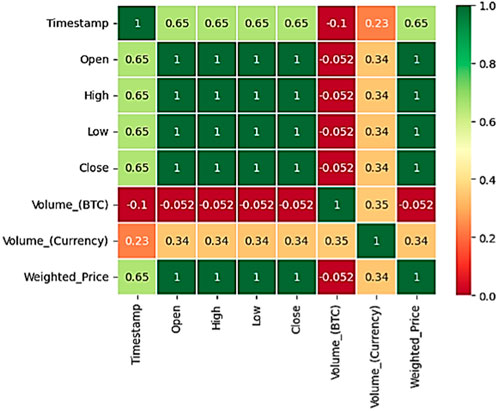
Figure 2. Correlation heatmap of Bitcoin data.
Achieving steady accurate forecasting in an uncertain price range requires the use of the variation point detection technique, which aids in the model’s adaptation to changes and fluctuations in the time series data. Every time a variation point is found, the predictive model has the ability to dynamically adjust its parameters or design to take into account the observed changes.
It covers the period from January 2012 to March 2021 and provides minute-by-minute apprises of OHLC (Open, High, Low, Close), volume in Bitcoin and the designated money, and the weighted price of Bitcoin. Both the opening and closing prices for a given day are shown in the Open and Close columns. The price for that day at its peak and lowest points are listed in the high and low columns, respectively. The volume column shows the total amount that was exchanged on a certain day. Traders utilise a trading benchmark called the “weighted price” to calculate the average weighted price, based on price and volume, at which an obligation has traded throughout the day. It is important since it informs traders about the value and movement of a security. For time series forecasting tasks, it is important to take into account several elements like the type of data, the particular problem being solved, and the available computational power when matching with deep learning models. Furthermore, the standard of the training data and hyperparameter adjustment can affect the model’s performance.
3.2 Exploratory data analysis
3.2.1 Augmented dickey-fuller (ADF) test
An approach to statistics known as the Augmented Dickey-Fuller (ADF) test is used to assess a time series’ stability. Stationarity is a key concept in time series analysis since most time series models and statistical techniques depend on the belief that the data is fixed. Time series data that has been fixed maintains statistical constants across time, such as its mean and variance. (Dahlberg, 2019). To determine if a unit root exists in a time series, the ADF test is frequently employed. A stochastic tendency in the time series, indicating that it is non-stationary. The ADF test helps determine whether differencing the series (i.e., computing the difference between consecutive observations) can make it motionless. The ADF trial involves regressing the time series on its lagged values and possibly on the differenced series. The test statistic is then computed, and its p-value is compared to the chosen significance level (Yousuf Javed et al., 2019). The ADF test uses various statistical software packages like Python (with libraries like StatsModels), R, or specialised econometrics software. Table 1 shows the Dickey-Fuller test result.
i. When the p-value is less than alpha, we cast off the possibility of a null and conclude that the data set is fixed.
ii. The series is non-stationary if the p-value is larger than or equal to alpha, which means that the null hypothesis cannot be rejected.
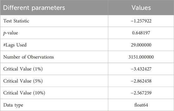
Table 1. Results of dickey-fuller test.
The null hypothesis in this instance is the only thing that differs from KPSS. The reality of a unit root, which recommends that the series is non-stationary, is the null premise of the test. Consequently, ADF claims that the series is stable. We deduced that the series is not motionless since KPSS asserts that it is not motionless (Brühl, 2020).
3.2.2 Auto correlation function (ACF)
A statistical technique called the Auto Correlation Function (ACF) is cast-off to calculate rapport among a time series and its own lagged version (Guesmi et al., 2019). Understanding patterns and temporal dependence in time series requires an understanding of this fundamental concept in time series evaluation. There is a correlation between the price at that lag and the present price if there is a positive autocorrelation at that particular lag. Trend identification may be aided by this information. For instance, a positive autocorrelation with a lag of one indicates that the price of the previous day and the present price are correlated. ACF is commonly rummage-sale in fields such as economics, finance, environmental science, and signal processing. Auto Correlation Function (ACF) is a beneficial implement for exploring temporal dependencies, identifying patterns, and understanding the behaviour of time series data (Miseviciute, 2018). The ACF for the Bitcoin weighted price is given in Figure 3. Determining noteworthy autocorrelation values and trends by analysing the ACF plot. Plot points that have peaks or troughs can provide information about the time series data’s underlying structure. Seasonality is a common occurrence in cryptocurrency markets, and it can be attributed to several factors like as trading patterns and market sentiment (Tripathy et al., 2022). ACF can be used to find patterns that reoccur at particular lags, suggesting that the data may be seasonal.
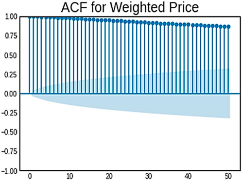
Figure 3. ACF for weighted price.
3.2.3 Partial auto correlation function (PACF)
In order to quantify the correlation among a time series and a lagged version of themselves while accounting for the impact of intermediate delays, time series analysts employ the Partial Auto Correlation Function (PACF), a statistical technique (Wu, 2021). In simple terms, PACF eliminates the impact of shorter delays by quantifying the direct association between data pieces at various time lags. When choosing the right variables for time series forecasting models, it can be helpful to understand the structure of the PACF. For example, adding certain lags to the model may enhance its prediction ability if there are notable partial autocorrelations at those precise lags. It is a crucial concept in understanding the temporal dependence and patterns within a time series, just like the Auto Correlation Function (ACF) (Mavridou et al., 2019). The PACF for the Bitcoin weighted price is given in Figure 4.
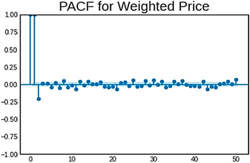
Figure 4. PACF for Bitcoin weighted price.
3.2.4 Visualizing using lag plots
Lag plots are a type of graphical technique used in data analysis and time series analysis to explore the autocorrelation or lagged relationships within a dataset (Zhang et al., 2021). They are particularly useful for understanding the temporal dependence or patterns in sequential data. Lagged plots are used to see the autocorrelation. They are crucial when utilising smoothing functions to modify the trend and stationarity (Lahmiri, 2021). The lag plot helps us understand the information more clearly. The lag plots of our dataset, which come with various time intervals, including 1-min, 1-h, daily, weekly, and 1-month are shown in Figure 5.
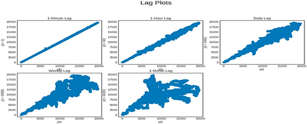
Figure 5. Lag plots.
3.3 Proposed methodology
The LSTM, FB-Prophet, Bi-LSTM, LSTM-GRU, and Silverkite algorithm models were some of the well-known models we employed. The Bi-LSTM outperformed others since the data were spatial-temporal and with other metrics explained in Section 4.
Data pre-processing is a critical stage in the pipeline for deep learning and data analysis. It entails organising, sanitising, and formatting raw data into a format that can be used for analysis or deep learning model training. The specific pre-processing steps we need to perform depend on the nature of our data. We present a framework for improved analysis. The framework is given in Figure 6.
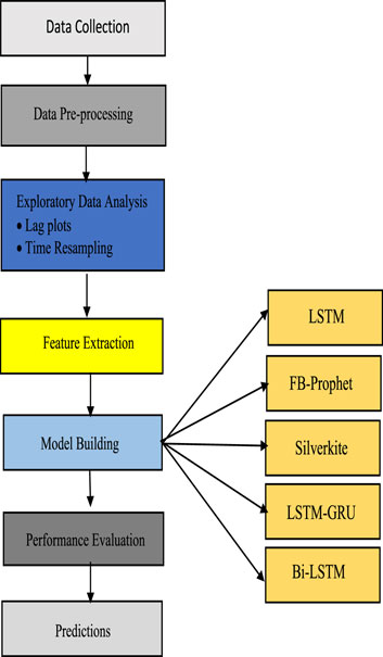
Figure 6. Overall workflow diagram.
3.4 Model building
3.4.1 LSTM
LSTMs are designed to overcome some of the confines of traditional RNNs when it comes to capturing and handling long-term dependencies in sequential data (Aljinović et al., 2021). The vanishing gradient problem limits RNNs’ efficacy in tasks involving dependencies over time by making it difficult for them to learn and remember information across lengthy sequences. Tasks requiring time series data, natural language processing, and additional data sequences with interdependent aspects are particularly well-suited for LSTMs. Unlike traditional RNNs, LSTMs can effectively handle the vanishing gradient problem, which often hinders the training of deep networks. LSTMs employ the hyperbolic tangent activation function (tanh) to process the values that flow through the memory cell (Rahmani Cherati et al., 2021). This function ensures that values are squashed between −1 and 1. An LSTM unit receives three vectors, or three lists of numbers, as input. At the previous instant (instant t-1), the LSTM produced two vectors that originate from the LSTM itself. Both the cell state (C) and the hidden state (H) are used in this. The third vector has an external source (Kądziołka, 2021). This is the vector X (also known as the input vector) that was sent to the LSTM at moment t. We are also using bidirectional LSTM in this work. An LSTM layer is wrapped in a bidirectional manner; we can choose the number of units and if we want the outputs at each time step. Figure 7 shows the simple LSTM architecture with cell state and hidden state. Eqs 1–5 show the simple LSTM model formulations.

Figure 7. LSTM architecture.
Input Gate–Selects the input value that will be cast-off to change the memory.
Where: σ = sigmoid activation function.
ht-1 = previous state.
Xt = input state.
Tanh = activation layer function.
Ct-1, Ct = cell state.
WC, Wi = weight matrix of input associated with hidden state
bc, bi = biases.
Forget gate–Decides which material should be removed from the memory.
Output gate–The output is determined by the input and memory of the block.
3.4.2 Bidirectional LSTM
In this study, we employ the Bi-LSTM model, which gathers information ranging from the past to the future by processing the input sequence in parallel from the beginning to the end. Future data will trigger adjustments to cell states and concealed states. The outputs from the forward and backward passes are frequently concatenated or combined to generate the Bi-LSTM layer’s final output. In the LSTM model and the conventional recurrent neural network model, information propagation is restricted to forward propagation, which means that the state at time t depends only on the information that existed before time t (Borst et al., 2018). To ensure that every instance has context information, Bidirectional Recurrent Neural Network (BiRNN) models and Long Short-Term Memory (LSTM) units are employed to record context. Figure 8 shows the basic bidirectional LSTM model architecture. Eqs 6–11 give the Bi-LSTM forward simplification, while Eqs 12–17 give the Bi-LSTM backward simplification.
• Forward LSTM equations
• Backward LSTM equations

Figure 8. Bi-LSTM architecture.
3.4.3 FB-prophet
Prophet was developed by the Facebook Core Data Science team, an open-source forecasting tool. It is specifically made for commercial and economic applications, with the ability to deal with time series data and produce precise forecasts. Prophet is renowned for being user-friendly and for its capacity to simulate holidays, special events, and seasonality in time series data. Time series data is broken down by Prophet into three primary categories: trend, fluctuations in demand, and holidays. The trends component shows how the data has grown or decreased over time, while the seasonality component accounts for recurring patterns. Holidays are included as special events that can affect the data (Kyriazis, 2020). Prophet is particularly popular in fields like retail, finance, and supply chain management, where accurate forecasting of time series data is essential for decision-making. It simplifies the process of time series forecasting and can be a valuable tool for analysts and data scientists working with historical data to make future predictions (Akyildirim et al., 2021). Eqs 18–20 stretch mathematical form of FB-prophet model. The additive regressive model on which FB Prophet’s prediction is built may be written as:
In (1), the error term is et, the trend factor is g(t), the holiday module is h(t), the seasonality component is s(t), and the additive regressive model is y(t). There are two techniques to model the trend factor g(t).
Logistic growth model: This model shows growth in multiple stages. In the early stages, development is roughly exponential; however, once the capacity is reached, it shifts to linear growth. The model may be written down as (2).
In this computational framework, L stands for the model’s maximum value, k for its growth rate, and x0 for its value at the sigmoid point.
Piece-wise linear model: This revised version of the linear model has separate linear relationships for the various ranges of x. The structure of the model can be expressed.
The breakpoint in the above model is x = c; (x-c) connects the two pieces of information; (x-c)+ is the interaction term, which is denoted by
3.4.4 LSTM-GRU
Ensemble models enhance overall performance by combining the predictions of several independent models and we can create an ensemble model using both LSTM and GRU networks. If both the LSTM and GRU models make similar errors, the ensemble may not be as effective. Experimentation and fine-tuning are essential to getting the best results with an ensemble of LSTM and GRU models (Wang et al., 2016). Ensemble models can often provide better performance than individual models because they leverage the strengths of each model and reduce their weaknesses. LSTM and GRU models can have different strengths in capturing patterns in sequential data, and combining them through an ensemble can lead to improved predictive performance. If both the LSTM and GRU models make similar errors, the ensemble may not be as effective. Experimentation and fine-tuning are essential to getting the best results with an ensemble of LSTM and GRU models.
The Cell Input state
Equations (21) and (22) explain how to use the sigmoid activation function to get a value between 0 and 1. Information retention and forgetting are controlled by the two variables
The information provided are modified after sources like. Equations (23) and (24) describe how
Information preservation is decided by
3.4.5 Silverkite
In order to make prediction for data scientists simpler, LinkedIn publishes the time-series forecasting library Greykite. Silverkite, an automated forecasting method, is the main forecasting algorithm utilised in this package. GrekKite was created by LinkedIn to assist its employees in making wise decisions based on time-series forecasting models. We provide a brief summary of the Silverkite model’s mathematical formulation in this section, assume that Y (t), where t represents time, is a real-valued time series with (t = 0, 1, ...). We use F (t) to represent the information that is currently accessible. F (t), for instance, can include other variables are Y (t-1), Y (t-2), X (t), and X (t- 1). The latter is sometimes called a delayed regressor. Y (t-i) signifies lags of Y; X (t) is the result of a regressor observed at time t, and X (t- 1) is the result of the similar regressor at time t-1. Eqs 31–35 give the Silverkite model conditional mean simplifications. The model of conditional mean is,
where G, S, H, A, R, and I are covariate functions in F (t). These variables or their interactions are combined linearly to create them. The overall growth term, G (t), may include the trend changepoints t1, ., tk, and as
where
where M is the series order
where
It might be lagged data, such as Y (t-1), ... , Y (t-r) for some order r, or an accumulation of wrapped annotations, like AVG (Y (t); 1, 2, 3) =
Other time series with the identical frequency as Y (t) that might usefully be used to forecast Y (t) are included in R(t). These time series are regressors, indicated by the symbols X (t) =
Assume that the objective series is Y (t) and the projected series is
The data can be used to determine an acceptable N (for instance, through cross-validation by examining the range of the residues). The prophecy interlude with close 1-
When this presumption is broken, Silverkite provides the option of building the prediction intervals using empirical quantiles. Due to Silverkite’s adaptability, more volatility models may be included. For instance, numerous characteristics, including continuous ones, might be conditional using a regression-based volatility model.
3.5 How Silverkite fulfils the conditions
The time series parameters described in Section 2 are handled by Silverkite. The Fourier series foundation function S (t) effectively captures strong seasonality. For the purpose of capturing intricate seasonality patterns, a higher-order M or categorical variable (such as the hour of day) can be utilised. By automatically identifying seasonality and trend changepoints, growth and seasonality changes across time are managed. Another advantage of autoregression, which is particularly helpful for short-term projections, is quick pattern alteration. We handle significant volatility during holidays and month/quarter borders by letting the variation in the model condition on such events and explicitly including their impacts in the mean model. Silverkite provides interactions between periodicity and holiday indicators in order to capture variations in seasonality throughout holidays. Greykite’s holiday database may be used to quickly find the dates of floating holidays. By eliminating known discrepancies from the training set, local abnormalities are managed. Regressors are used to account for the impact of outside influences; their anticipated values may originate from Silverkite or another model. This makes it possible to contrast forecasting possibilities. As a result, Silverkite’s design intuitively captures certain time series properties that are conducive to modelling and understanding.
4 Discussion
In general, we separate the Bitcoin time series data in to training and validation intervals in order to assess the forecasting model’s accuracy. For validation, we selected a patch of data spanning from July 2020 to March 2021, which is 10% of the overall data set. It is known as fixed partitioning. During the training phase, we will train our model, and during the validation phase, we will assess it. This is the area where we conduct experiments to determine the best training architecture. Continue adjusting it and other hyperparameters until we achieve the necessary performance, as determined by the validation set (Kim et al., 2018). Following that, one may often use either the validation and training data to retrain the system. Next, assess our model in the test (or prediction) phase to see whether it performs similarly. If it succeeds, we may try the new approach of using the test data to retrain again. The test data is the set of data that most closely resembles the current situation. If our model was not trained with similar data as well, it might not perform as well (Shokoohi-Yekta et al., 2017).
Figure 9 displays the library that supports the forecast procedure at every stage. We use a sort of recurrent neural network architecture called Bidirectional LSTM (BiLSTM), which is especially well-suited for sequence processing applications. It is an extension of the traditional LSTM (Long Short-Term Memory) network. In a standard LSTM, information flows in one direction through the network, from the input sequence’s beginning to its end. On the other hand, Bi-LSTM analyses the order of inputs in two different ways: forward, from the start of the sequence to the end, and backward, from the conclusion to the beginning. The network is better able to comprehend sequential input because of its bidirectional processing, which enables it to record relationships across the past as well as the future setting during each time step.
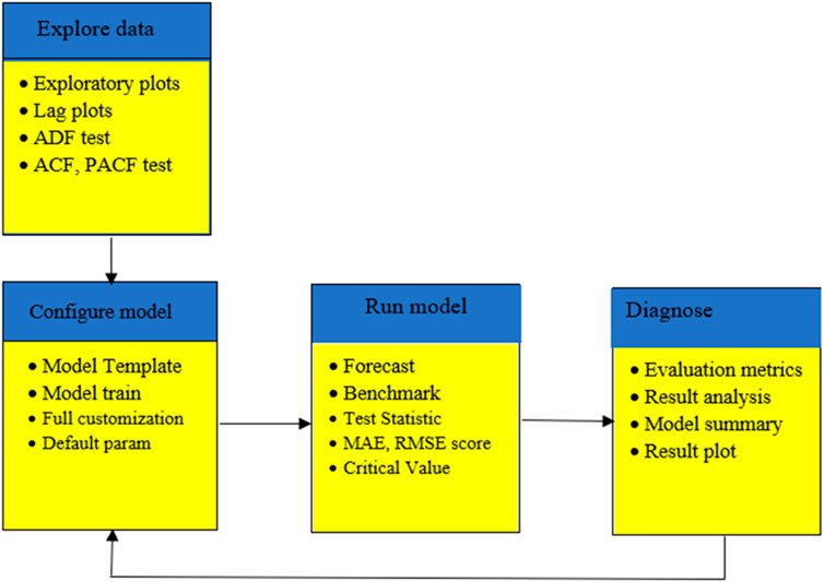
Figure 9. Library supports the forecast workflow at every stage.
In this part, results and evaluation on the test dataset are shown graphically. The months and the overall price rate are represented by the x and y-axes in Figure 10, which shows the LSTM predicted Bitcoin price. Figures 11, 12 shows the FB-Prophet and Silverkite predicted BTC price, respectively. Figures 13, 14 shows the LSTM-GRU and Bidirectional-LSTM predicted BTC price. The test data for this collection was collected between July 2020 and March 2021. Dealing with time-series data can show a lot when it is visualised. Markers can be placed on the plot to help emphasise particular observations or events in the time series. Traders are always looking for ways to profit from opportunities since the market for digital currencies is always open and cryptocurrencies are susceptible to huge price swings. Trading professionals can select when to buy or sell by visualising the weighted price.
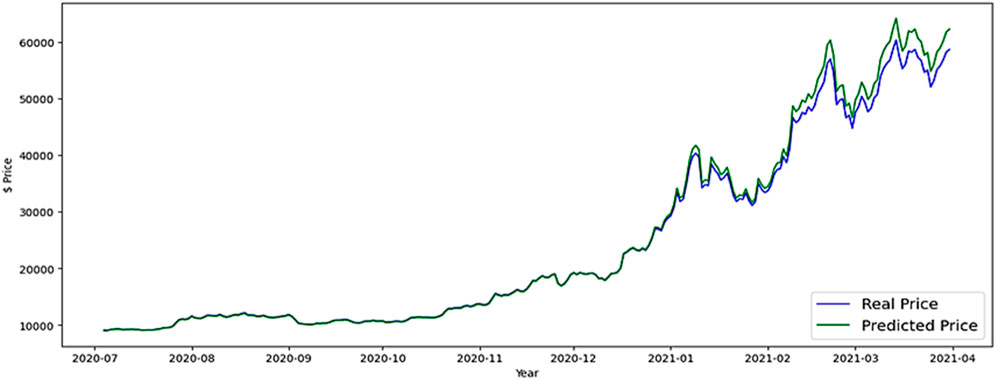
Figure 10. LSTM forecast BTC price.
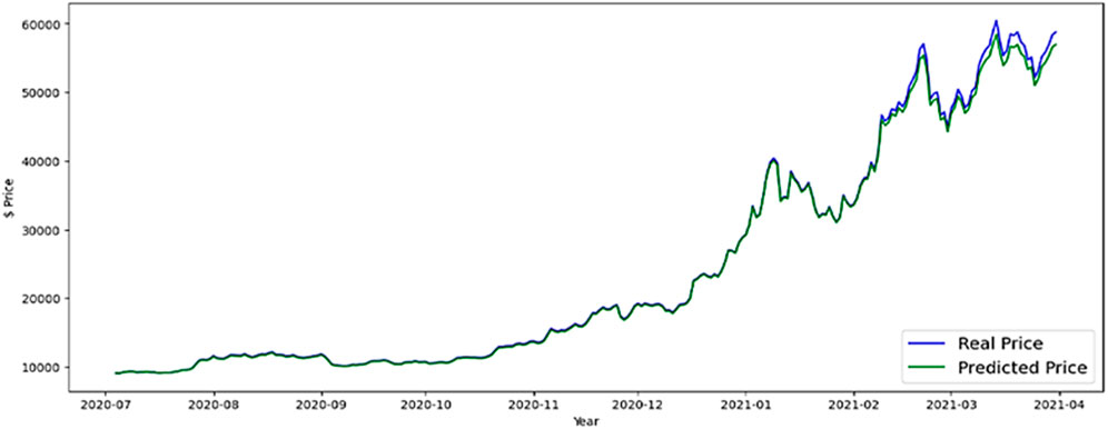
Figure 11. FB-Prophet forecast BTC price.
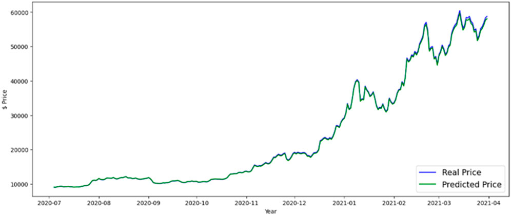
Figure 12. Silverkite forecast BTC price.
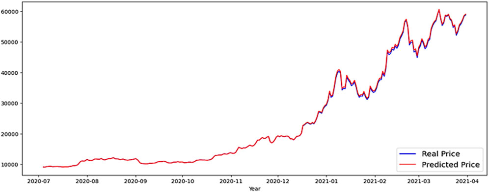
Figure 13. LSTM-GRU forecast BTC price.
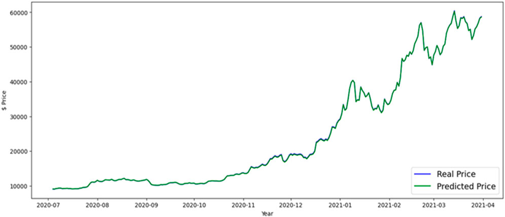
Figure 14. Bi-LSTM forecast BTC price.
The majority of LinkedIn’s projections up to this point were corporal, ad hoc, and intuition-based. Customers across all business sectors and engineering are already embracing algorithmic forecasting. Customers are aware of the advantages of precision, scope, and consistency. Our projections help LinkedIn prepare and respond quickly to new information by saving time and bringing clarity to the business and infrastructure. This culture change was made possible by a family of models that are quick, adaptable, and easy to comprehend, as well as by a modelling framework that makes self-serve forecasting simple and accurate.
Asset managers and regular investors alike need to forecast the cost of bitcoin (Sharma, 2018). Because Bitcoin is money, it cannot be analysed in the same manner as other traditional currencies. In the case of conventional currencies, key economic theories include uncovered interest rate parity, parity of buying power, and cash flow projection models. This is because the digital currency market, such as Bitcoin, makes it impossible to use some traditional guidelines on supply and demand. On the other hand, a number of characteristics of Bitcoin, such as its speedy transactions, diversity, decentralisation, and the enormous worldwide network of individuals interested in discussing and expressing important information on digital currencies, notably Bitcoin, make it advantageous to shareholders (Tripathy et al., 2024).
5 Result analysis
Right out of the box, the Bi-LSTM model exhibits good performance on data that is internal as well as external, with intervals coming from a range of domains. Its adaptable architecture enables variables, the goal function, and the volatility model to be fine-tuned. We anticipate that forecasters will find the free Greykite library to be especially helpful when dealing with time series that have features, such as time-dependent expansion and seasonality, holiday impacts, anomalies, and/or reliance on outward causes, mutual of time series pertaining to social activity. We rapidly compare our newly proposed strategy with the results of previous research in the sector. Table 2 confirms that the RMSE value for the LSTM is 5.670, whereas the principles for the FB-Prophet, Silverkite, LSTM-GRU and Bidirectional-LSTM(Bi-LSTM) are 2.573, 2.473, 0.917 and 0.815 respectively. Overall, the suggested forecasting model Bi-LSTM result is significant as compared to others. Table 2 we take the error score of each model. The histogram plot of the MAE, MSE and RMSE scores is shown in Figure 15.
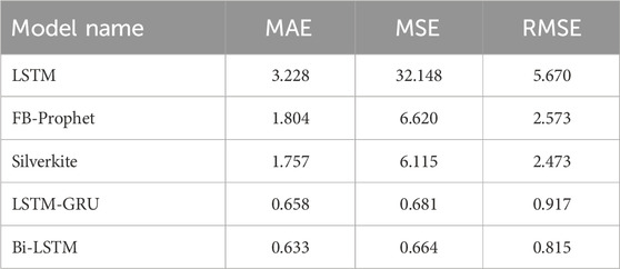
Table 2. Error score of each model.
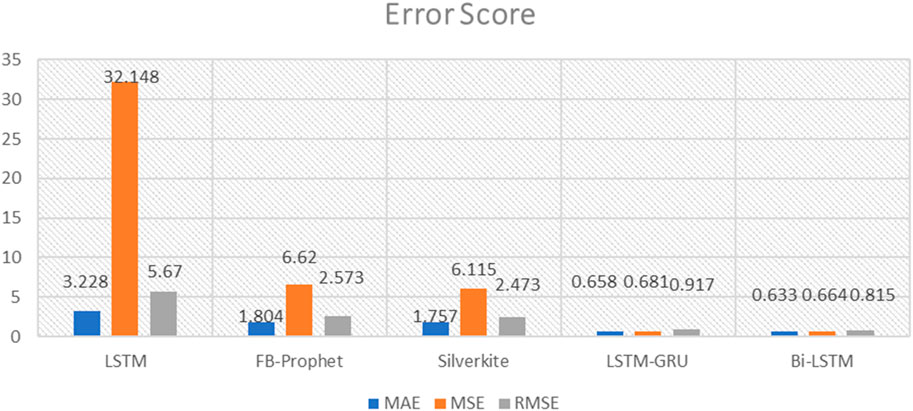
Figure 15. Histogram plot of the MAE, MSE, and RMSE score.
6 Conclusion
While Bitcoin price prediction models and tools can be informative, it is important to approach them with caution and consider them as one of many factors when making financial decisions in the cryptocurrency market. The intervals originating from multiple domains and ranging from hourly to monthly, Bidirectional-LSTM (Bi-LSTM) model works well on internal as well as external datasets right out of the box. Bidirectional wraps an LSTM layer, and we can specify the number of units, whether we want the outputs at each time step (return_sequences = True), and other parameters as needed. The objective function and the volatility model may be adjusted thanks to its adaptive architecture. We believe that forecasters will find the free Greykite library to be particularly useful when working with time series. Bitcoin has experienced significant growth and gained popularity as a digital asset. Its volatility means that it can experience rapid price fluctuations. When making investments in Bitcoin or a different cryptocurrency, investors should think about their risk tolerance, spread their portfolios, and do extensive research.
Additionally, consulting with financial advisors and staying informed about the latest developments in the cryptocurrency market is advisable for those considering Bitcoin as an investment. The prediction rate for bitcoin may be increased in the future by further optimising deep learning models utilising additional self-adaptive approaches and linking them to the price and behaviour of crypto assets. Researchers can utilize the forecasted data to gain deeper insight into the workings of the bitcoin market. This could lead to a better understanding of the factors behind price fluctuations. Forecasting results can be used to analyze market sentiment and public opinion toward specific cryptocurrencies. Plans for marketing and public relations initiatives could find this material helpful. Accurate forecasting helps investors and traders assess and manage the risks associated with bitcoin transactions. When people forecast price swings, they may make informed decisions about what to buy, sell, or hold onto.
Data availability statement
The original contributions presented in the study are included in the article/supplementary material, further inquiries can be directed to the corresponding author.
Author contributions
NT: Conceptualization, Data curation, Formal Analysis, Funding acquisition, Investigation, Methodology, Project administration, Resources, Software, Supervision, Validation, Visualization, Writing–original draft. SN: Data curation, Formal Analysis, Investigation, Supervision, Validation, Visualization, Writing–review and editing. SP: Conceptualization, Formal Analysis, Methodology, Supervision, Validation, Writing–review and editing.
Funding
The author(s) declare that no financial support was received for the research, authorship, and/or publication of this article.
Conflict of interest
The authors declare that the research was conducted in the absence of any commercial or financial relationships that could be construed as a potential conflict of interest.
Publisher’s note
All claims expressed in this article are solely those of the authors and do not necessarily represent those of their affiliated organizations, or those of the publisher, the editors and the reviewers. Any product that may be evaluated in this article, or claim that may be made by its manufacturer, is not guaranteed or endorsed by the publisher.
References
Akyildirim, E., Aysan, A. F., Cepni, O., and Darendeli, S. P. C. (2021). Do investor sentiments drive cryptocurrency prices? Econ. Lett. 206, 109980. doi:10.1016/j.econlet.2021.109980
Aljinović, Z., Marasović, B., and Šestanović, T. (2021). Cryptocurrency portfolio selection—a multicriteria approach. Mathematics 9 (14), 1677. doi:10.3390/math9141677
Borst, I., Moser, C., and Ferguson, J. (2018). From friendfunding to crowdfunding: relevance of relationships, social media, and platform activities to crowdfunding performance. New Media Soc. 20 (4), 1396–1414. doi:10.1177/1461444817694599
Brühl, V. (2020). Libra - a differentiated view on facebook’s virtual currency Project. Intereconomics 55 (1), 54–61. doi:10.1007/s10272-020-0869-1
Dahlberg, T. (2019). What blockhain developers and users expect from virtual currency regulations: a survey study. IP 24 (4), 453–467. doi:10.3233/ip-190145
Guesmi, K., Saadi, S., and Abid, I. (2019). Portfolio diversification with virtual currency: evidence from bitcoin. Int. Rev. Financ. Anal. 63, 431–437. doi:10.1016/j.irfa.2018.03.004
Guindy, M. A. (2021). Cryptocurrency price volatility and investor attention. Int. Rev. Econ. Finance 76 (1), 556–570. doi:10.1016/j.iref.2021.06.007
Guo, H., Hao, L., Mukhopadhyay, T., and Sun, D. (2019). Selling virtual currency in digital games: implications for gameplay and social welfare. Inf. Syst. Res. 30 (2), 430–446. doi:10.1287/isre.2018.0812
Ji, S., Kim, J., and Im, H. (2019). A comparative study of bitcoin price prediction using deep learning. Mathematics 7 (10), 898. doi:10.3390/math7100898
Kądziołka, K. (2021). The promethee II method in multi-criteria evaluation of cryptocurrency exchanges. Econ. Reg. Studies/Studia Ekon. i Reg. 14 (2), 131–145. doi:10.2478/ers-2021-0010
Keogh, E., Chakrabarti, K., Pazzani, M., and Mehrotra, S. (2001). Dimensionality reduction for fast similarity search in large time series databases. Knowl. Inf. Syst. 3 (3), 263–286. doi:10.1007/pl00011669
Kim, S., Lee, H., Ko, H., Jeong, S., Byun, H., and Oh, K. (2018). Pattern matching trading system based on the dynamic time warping algorithm. Sustainability 10 (12), 4641. doi:10.3390/su10124641
Kyriazis, N. A. (2020). Herding behaviour in digital currency markets: an integrated survey and empirical estimation. Heliyon 6 (8), e04752. doi:10.1016/j.heliyon.2020.e04752
Lahmiri, S. (2021). Deep learning forecasting in cryptocurrency high-frequency trading. Cogn. Comput. 13 (2), 485–487. doi:10.1007/s12559-021-09841-w
Lamothe-Fernández, P., Alaminos, D., Lamothe-López, P., and Fernández-Gámez, M. A. (2020). Deep learning methods for modeling bitcoin price. Mathematics 8 (8), 1245. doi:10.3390/math8081245
Liu, S. (2019). Recognition of virtual currency sales revenue of online game companies. Acad. J. Humanit. Soc. Sci. 2 (7), 29–36. doi:10.25236/AJHSS.2019.020704
Livieris, I. E., Pintelas, E., Stavroyiannis, S., and Pintelas, P. (2020). Ensemble deep learning models for forecasting cryptocurrency time-series. Algorithms 13 (5), 121. doi:10.3390/a13050121
Mavridou, A., Laszka, A., Stachtiari, E., and Dubey, A. (2019). “Verisolid: correct-bydesign smart contracts for ethereum,” in international conference on financial cryptography and data security (Springer), 446–465.
McNally, S., Roche, J., and Caton, S. (2018). “Predicting the price of bitcoin using machine learning,” in 2018 26th euro micro international conference on parallel, distributed and network-based processing (PDP) (IEEE), 339–343.
Miseviciute, J. (2018). Blockchain and virtual currency regulation in the EU. J. Invest. Compliance 19, 33–38. doi:10.1108/joic-04-2018-0026
Putra, P., Jayadi, R., and Steven, I. (2021). The impact of quality and price on the loyalty of electronic money users: empirical evidence from Indonesia. J. Asian Finance Econ. Bus. 8 (3), 1349–1359. doi:10.13106/jafeb.2021.vol8.no3.1349
Rahmani Cherati, M., Haeri, A., and Ghannadpour, S. F. (2021). Cryptocurrency direction forecasting using deep learning algorithms. J. Stat. Comput. Simul. 91, 2475–2489. doi:10.1080/00949655.2021.1899179
Rosenfeld, R., Lakatos, A., Beam, D., Carlson, J., Flax, N., Niehoff, P., et al. (2018). Commodity futures trading commission issues advisory for virtual currency pump-and-dump schemes. J. Invest. Compliance 19, 42–44. doi:10.1108/JOIC-04-2018-0033
Sharma, A. (2018). On the exploration of information from the DTW cost matrix for online signature verification. IEEE Trans. Cybern. 48 (2), 611–624. doi:10.1109/TCYB.2017.2647826
Shokoohi-Yekta, M., Hu, B., Jin, H., Wang, J., and Keogh, E. (2017). Generalizing DTW to the multi-dimensional case requires an adaptive approach. Data Min. Knowl. Disc 31 (1), 1–31. doi:10.1007/s10618-016-0455-0
Tripathy, N., Hota, S., and Mishra, D. (2023a). Performance analysis of bitcoin forecasting using deep learning techniques. Indonesian J. Electr. Eng. Comput. Sci. 31 (3), 1515–1522. doi:10.11591/ijeecs.v31.i3.pp1515-1522
Tripathy, N., Hota, S., Mishra, D., Satapathy, P., and Empirical, N. S. K. (2024). Forecasting analysis of bitcoin prices: a comparison of machine learning, deep learning, and ensemble learning models. Int. J. Electr. Comput. Eng. Syst. 15 (1), 21–29. doi:10.32985/ijeces.15.1.3
Tripathy, N., Hota., S., Prusty, S., and Nayak, S. K. (2023b). “Performance analysis of deep learning techniques for time series forecasting,” in International Conference in Advances in Power, Signal, and Information Technology, 639–644.
Tripathy, N., Nayak, S. K., Godslove, J. F., Friday, I. K., and Dalai, S. S. (2022). Credit card fraud detection using logistic regression and synthetic minority oversampling technique (SMOTE) approach. Technology 8 (4), 4.
Wang, D., Gao, X., and Wang, X. (2016). Semi-supervised nonnegative matrix factorization via constraint propagation. IEEE Trans. Cybern. 46 (1), 233–244. doi:10.1109/TCYB.2015.2399533
Window, Wu. C. (2021). Effect with markov-switching GARCH model in cryptocurrency market. Chaos. Solit. Fractals 146, 110902. doi:10.1016/j.chaos.2021.110902
Xu, Z., and Tang, C. (2021). Challenges and opportunities in the application of China’s central bank digital currency to the payment and settle account system. Fin 9 (4), 233. doi:10.18282/ff.v9i4.1553
Yousuf Javed., M., Husain, R., Khan, B. M., and Azam, M. K. (2019). Crypto-currency: is the future dark or bright? J. Inf. Optim. Sci. 40 (5), 1081–1095. doi:10.1080/02522667.2019.1641894
Keywords: cryptocurrency, LSTM, Fb-prophet, LSTM-GRU, Silverkite, bidirectional-LSTM, forecasting, time series analysis
Citation: Tripathy N, Nayak SK and Prusty S (2024) A comparative analysis of Silverkite and inter-dependent deep learning models for bitcoin price prediction. Front. Blockchain 7:1346410. doi: 10.3389/fbloc.2024.1346410
Received: 29 November 2023; Accepted: 29 February 2024;
Published: 28 May 2024.
Edited by:
Rachid Elazouzi, University of Avignon, FranceReviewed by:
Anupama Mishra, Swami Rama Himalayan University, IndiaRoseline Oluwaseun Ogundokun, Landmark University, Nigeria
Copyright © 2024 Tripathy, Nayak and Prusty. This is an open-access article distributed under the terms of the Creative Commons Attribution License (CC BY). The use, distribution or reproduction in other forums is permitted, provided the original author(s) and the copyright owner(s) are credited and that the original publication in this journal is cited, in accordance with accepted academic practice. No use, distribution or reproduction is permitted which does not comply with these terms.
*Correspondence: Nrusingha Tripathy, nrusinghatripathy654@gmail.com