The effect of site exposure index on the required capacities of aquaculture structures

This study investigates the relationship between an ocean site's Exposure Index and the required capacity of finfish, shellfish, and seaweed aquaculture structures. This study provides insights into the efficacy of combining the design significant wave height, peak periods, horizontal wave orbital velocity amplitudes, horizontal current speeds, and water depth into a single index representing exposure. The research builds upon exposure indices proposed previously, and uses Hydro-/Structural Dynamic Finite Element Analysis (HS-DFEA) to quantify the required structural capacities for cultivation structures as a function of exposure index based on representative sites in the German Bight of the North Sea. The selection of 36 sites in this region was based on extreme hydrodynamic and mean bathymetric conditions, utilizing a k-means clustering approach to identify a collection of sites within a broad range of environmental conditions. Through a detailed analysis of the dynamic simulations of each farm type under 50-year storm conditions, we calculated the required capacities of each system for each site. We then evaluated the performance of significant wave height, depth, distance to shore, and the proposed exposure indices as linear predictors of the normalized required capacities. No meaningful linear relationship existed between structural loads and water depth or distance to the nearest coastline. While there is still uncertainty about the utility of exposure indices as a linear predictor of structural loads, this research found that Exposure Velocity was the best linear predictor across structure types by a slim margin, followed closely by the Specific Exposure Energy, Exposure Velocity at a Reference Depth of 5 m, and the Structure-centered Drag-to-Buoyancy Ratio ($R^2$ = 0.69, 0.61, 0.60, 0.60 respectively). This investigation indicates that these exposure indices can be used to communicate what physical ocean conditions mean for an aquaculture structure's required capacity.

1 Introduction

Aquaculture is the fastest growing animal food production sector in the world (FAO et al., 2020). It has the potential to be sustainable and environmentally friendly compared to land-based agriculture (Nijdam et al., 2012; Gephart et al., 2014; Troell et al., 2014) and even has major ecological benefits (Theuerkauf et al., 2022). Aquaculture is a proven alternative to conventional capture fisheries and can become a stable economic engine for coastal communities that have had to deal with overfishing (Hilborn and Hilborn, 2012), ocean warming (Oremus, 2019), acidification (Byrne, 2011), more restrictive catch quotas (NOAA, 2017), and declines in migrating species (Limburg and Waldman, 2009).

Technologies and production methods for nearshore aquaculture exist, but suitable sites in protected waters are limited (Marra, 2005; Duarte et al., 2009; Sanchez-Jerez et al., 2016). There is a significant opportunity and necessity to expand aquaculture in the open ocean. According to National Institute of Standards and Technology, if industrial scale offshore production could be achieved, the farm gate value would be approximately $1.5–2B USD (Browdy and Hargreaves, 2009). In response to the the potential benefits, NOAA Fisheries developed a permitting process for developing open-ocean aquaculture in the Gulf of Mexico (NOAA, 2016).

However, the costs of venturing into large-scale offshore operations will be substantial, involving considerable upfront capital expenditure typically driven by the required structural capacities of mariculture structures. To support new ventures in aquaculture and ensure sound site selection, the levelized cost of production must be considered. Earlier insights into the challenges of “offshore aquaculture” or site exposure point to the importance of water depth, significant wave height, and distance from the coast (Ryan, 2004; Lovatelli et al., 2013; Froehlich et al., 2017). Site suitability studies, which often are based on a Geographic Information System, account for socio-economic and marine use constraints, distance from a port or harbor, environmental impact, applicable biological and physical ocean conditions for growth, species and structure survival, and farm operations (Falconer et al., 2013; Puniwai et al., 2014; Porporato et al., 2020). The mariculture structure technology for exposed offshore environments is still in development (Goseberg et al., 2017; Moscicki et al., 2024) and a generalized relationship between the required structural capacities of mariculture structures and the physical characteristics that define a site (e.g. depth, current velocity, wave environments) is not defined. Defining this relationship in a digestible manner supports site suitability studies as well as estimates of capital expenditures associated with aquaculture structures.

Lojek et al. (2024) developed and presented six different indices (“exposure indices”) to quantify the hydrodynamic exposure of various ocean sites, combining the effects of current velocity, significant wave height, peak wave period, depth, and structure characteristics into single characteristic values. Therein, extreme exposure indices with a 50-year return period were spatially evaluated within the German Bight of the North Sea using data products obtained from the EasyGSH-DB portal (Hagen et al., 2021; Sievers et al., 2021; www.easygsh-db.org). However, no relationship between 50-year exposure indices and the resultant structural loads on aquaculture structures was investigated. Defining how the proposed exposure indices relate to required structural capacities is necessary to understand their utility. To address this gap in knowledge, this study investigates the relationship between the required structural capacities and exposure indices across a range of exposed sites and a series of aquaculture structures.

This study places emphasis on understanding if an exposure index is approximately proportional to maximum loads on an aquaculture structure; the existence of this quality supports both (a) the utility of the exposure index and (b) its interpretability by subject matter experts and non-experts alike. This research demonstrates that select exposure indices can effectively quantify ocean site exposure and its implication for the required capacity of aquaculture structures through a linear relationship. While this approach provides a general and accessible framework, there remains uncertainty in the relationship.

This manuscript is one of a suite of papers compiling a Research Topic, “Differentiating and defining ‘exposed’ and ‘offshore’ aquaculture and implications for aquaculture operation, management, costs, and policy”. The Research Topic includes manuscripts focused on aquaculture policy and regulation in marine environments, the definitions of terms regarding aquaculture in marine systems, the derivation of the energy index, trends required to advance aquaculture into high energy marine zones, costs and implications in aquaculture of using the index and social science aspects relating to marine aquaculture (Buck et al., 2024).

2 Materials and methods

The proposed exposure indices in Lojek et al. (2024) each provide an indication of any ocean site's exposure to hydrodynamic energy or forcing. In the present study, we aim to evaluate the relationship between extreme 50-year exposure indices and design mooring line loads (proportional to the required capacity) of select mussel, macroalgae, and finfish aquaculture structures. Here, we evaluate relationships between exposure indices and mooring line capacities at representative sites in the German Bight of the North Sea by:

1. Selection of representative physical ocean conditions at aquaculture sites (n=36) through a k-means clustering approach,

2. Engineering design of aquaculture cultivation structures at each site with common geometries across structure types characterized by a 200-meter-long mussel backbone growline, a 38 m by 187m tensioned macroalgae array, and a 12 m diameter and 6 m deep finfish net pen,

3. Hydro-/Structural-Dynamic Finite Element Analysis (HS-DFEA) numerical modeling of the aquaculture structures under static calm-water and dynamic extreme load cases,

4. Calculation of the normalized required capacity of each aquaculture structure,

5. Calculation of the extreme values of exposure indices, and

6. Linear regression of (i) normalized required capacity on each of the parameters that previously designated sites as “offshore” and (ii) normalized required capacity on each of the extreme exposure indices.

2.1 Definition of hydrodynamic variables and exposure indices

Lojek et al. (2024) developed and proposed six exposure indices: Exposure Velocity (EV), Exposure Velocity at a Reference Depth (EVRD), Specific Exposure Energy (SEE), Depth-integrated Energy Flux (DEF), Structure-centered Depth-integrated Energy (SDE), Structure-centered Drag-to-Buoyancy Ratio (SDBR). Definitions of exposure indices consider (i) hydrodynamic variables describing design waves, currents, and depths and (ii) structural properties such as characteristic diameter or solidity. For the derivation and further description of each exposure index, readers are directed to Lojek et al (2024), Section 2.

Hydrodynamic variables considered in the definition of exposure indices include: vertical position $z$ (positive up), depth $d$ ($d=-z$ at seabed), horizontal current velocity $\stackrel{\rightharpoonup }{U_c}(z)$ and speed $U_c(z)=\parallel \stackrel{\rightharpoonup }{U_c}{(z)}_2\parallel$, significant wave height $H_s$, peak wave period $T_p$, wave energy period $T_E$, horizontal wave orbital velocity amplitude $u_w(z)=\frac{\pi H}{T}\frac{\cosh k(z+d)}{\sinh kd}$ (in application, $H_s=H$ and $T=T_p$). Structure based variables include: non-dimensional structural component solidity S, structural component surface area surface area $A_{structure}$, structural component characteristic length $D$. Assumed constants in application include seawater density, $\rho$, and gravitational acceleration, $g$.

Of these metrics, EV, EVRD, SEE, and DEF are independent of structural properties, whereas SDE and SDBR incorporate the structural components characteristics. The EV and EVRD (or EV at a depth of 5 m),

$\begin{array}{ll}EV= U_c(z)+u_w(z)& (1)\end{array}$

$\begin{array}{ll}EVRD=U_{c5}+u_{w5}& (2)\end{array}$

have units of distance per unit time and were proposed to take into account the loads on aquaculture structures depend on the combined current and wave-induced fluid speeds. The SEE,

$\begin{array}{ll}SEE=1/2 {(U_c(z) + u_w(z))}^2& (3)\end{array}$

which has units of energy per unit mass, was constructed to be proportional to the square of the sum of current and wave-induced fluid velocity, which is proportional to the drag force in the classical drag equation. The DEF,

$\begin{array}{ll}DEF= \frac{\rho g^2(H_s^2)T_E}{64\pi }+ \frac{1}{2}\rho d{(U_c)}^3& (4)\end{array}$

has units of power per unit distance and was adapted from measures of wave- and current-energy flux used in marine renewable energy applications. The structure-dependent SDE,

$\begin{array}{ll}SDE=(1/8·g·{H_s}^2+1/2·d·U^2 )·\rho ·S·A_{structure}& (5)\end{array}$

has units of energy times mass per volume and integrates wave and current energy from the seafloor to the water surface. The SDBR,

$\begin{array}{ll}SDBR=\frac{U^2}{2gD}& (6)\end{array}$

is a non-dimensional number to represent the ratio of drag forces to buoyancy forces on a structure, using classical equations for a slender cylinder.

2.2 Study area characterization: German Bight of the North Sea

2.2.1 Study area description

The nearshore and coastal ocean of the German Bight of the North Sea (Figure 1) is characterized by tidal and atmospheric forcing from the North Sea and North Atlantic Ocean connection, which interact over a shallow, gently sloping seabed and within the estuaries, tidal inlets, and ~10 km wide intertidal mudflats of the Wadden Sea along the coast. Low pressure systems of winter storms in the North Sea produce storm surges and energetic wind waves in the German Bight. Oscillations in tidal currents and water levels, which enter through the Strait of Dover in the southwest and through an open-ocean connection in the northwest, are non-linear and reflect a co-oscillating response (Hagen et al., 2020). Semidiurnal tides dominate, with currents that propagate counter-clockwise about the German Bight and are deflected towards the coast, reaching maximum amplitudes in the center of estuarine channels (Hagen et al., 2020). Residual tidal circulation forms a counter-clockwise pattern along the German Bight coastline (Klein and Frohse, 2008). Variations in sea surface temperatures and salinity in the German Bight generally follow a positive and negative land-to-sea cross shore gradient respectively, driven from continental river run-off and the atmospheric warming of the shallow waters of the Wadden Sea. On shorter time scales of 1 to 10 days, fronts with a length scale of 5 to 20 km are observed and are known to concentrate the density of marine life.

Figure 1

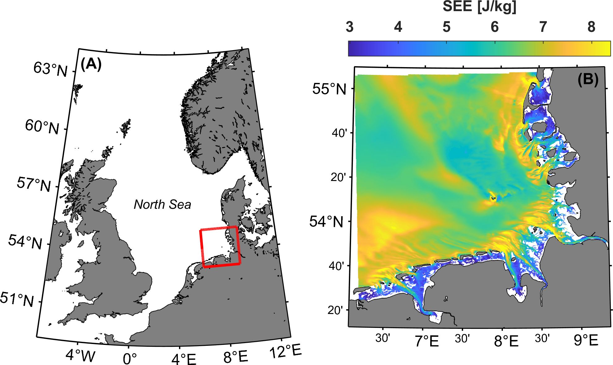
Figure 1. The (A) North Sea and German Bight study area (red box) in relation to (B) the computed 50-year Specific Exposure Energy (SEE). Adapted from Lojek et al. (2024). Graphic made with M_Map (Pawlowicz, 2020) with data products from Hagen et al. (2020), Sievers et al. (2020) and Wessel and Smith (1996).

Aquaculture within the German Bight is primarily focused on shellfish cultivation of mussels and oysters (Clawson et al., 2022). Scientific case studies have demonstrated that the German Bight is a suitable region for the cultivation of macroalgae (Buck, 2007). Historically, finfish aquaculture is not a common practice due to the regions extreme hydrodynamic conditions and shallow nearshore depths (Rosenthal and Hilge, 2000). However, future expansion into open ocean regions further from shore may be facilitated through the development of new technologies and co-location with offshore wind farms (Buck et al., 2018). Constructed, commissioned, and planned offshore wind park areas within the German Bight are available in Hannemann (2024) to provide further context to the body of literature that discusses multi-use concepts involving offshore wind and aquaculture production (Buck et al., 2008; Gimpel et al., 2015; Buck and Langan, 2017; Przedrzymirska et al., 2021).

2.2.2 High-resolution regional datasets

The characterization of surface currents, significant wave heights and associated peak periods, and mean depths follows that of Lojek et al. (2024). Analysis of hydrodynamic parameters was facilitated through EasyGSH-DB. EasyGSH-DB maintains open access to a 20-year 100 m gridded dataset of bathymetry, 100 m gridded wave parameters, and 1 km depth averaged current velocities in the German Bight—the latter two are derived from a spectral wave model hindcast and a 3D regional ocean model hindcast, respectively (Hagen et al., 2021). The EasyGSH-DB products (Hagen et al., 2020; Sievers et al., 2020) and metadata were obtained from the EasyGSH-DB portal (www.easygsh-db.org).

2.2.3 Extreme values of hydrodynamic parameters

Univariate extreme value analysis of significant wave heights and depth averaged current speeds follows that of Lojek et al. (2024), who fit series of annual maxima to the Gumbel distribution to derive extreme values at the 2% exceedance probability (50-year return period) for each parameter. The 50-year depth averaged current speeds were interpolated to the same 100 m grid as $H_s$ and bathymetry, using linear interpolation throughout most of the domain and nearest neighbor interpolation along the coastline. 50-year surface current speeds were estimated from 50-year depth average current speeds by assuming current profiles followed a power law in the vertical with an exponent of 1/7 and no-slip at the bottom boundary.

2.3 Aquaculture site selection

To ensure that the breadth of possible site characteristics was considered, a subset of important hydrodynamic variables were sampled and used as criteria for representative site selection. The objective of aquaculture site selection was to define a representative subset of hydrodynamic variables that exist within the German Bight. The authors acknowledge the site selection methodology does not represent the full breadth of hydrodynamic variables that coexist in the coastal ocean.

A set of 36 representative sites across the German Bight were selected from the 100 m regular gridded values of extreme hydrodynamic variables and mean depth. Variables considered include (1) significant wave height $H_S$, (2) peak wave period $T_p$, (3) horizontal wave orbital velocity amplitude $u_w$, (4) horizontal current speed $u_c$, and (5) water depth $d$ at mean sea level. Selected hydrodynamic variables were used both in the evaluation of exposure indices (e.g. Specific Exposure Energy, Figure 1) and in load cases for numerical simulation of aquaculture cultivation structures.

The selection of 36 representative sites in the 5D parameter space $C$ with dimensions corresponding to variables (1)–(5) was achieved through k-means clustering in two discrete phases. The k-means algorithm seeks to identify clusters in an n-dimensional variable space by grouping (or clustering) data such that the sum of within-cluster variances is minimized (Hartigan and Wong, 1979). Each variable $x\in C$ was normalized by its mean $\mu$ and standard deviation $\sigma$ , to define $x_n=\frac{x-\mu }{\sigma }$ such that equal scales of variables are considered against one another when computing the sum of variances in the k-means algorithm. The centroid of each identified cluster in the normalized variable space was then transformed back into the original variable space by multiplying centroids by σ and then adding μ. This implementation of the k-means algorithm does not explicitly account for spatial autocorrelation, since it does not directly consider the spatial arrangement of data points. In the first phase, the selection process considered all points with depths greater than 10 m. In the second phase, sites reflecting lower energy regions that were at least 1.5 km away from the coast were selected through k-means clustering of a subset of $C$ defined by all locations where the horizontal wave orbital velocity amplitude and the horizontal current speed $$ were below their respective 5^th quantiles and a relaxed minimum depth of 7 m.

The cluster centroids, or the mean value of each cluster, are shown in Figure 2 with respect to $C$ . The representative locations of each cluster defining the 36 sites are overlaid on maps of each key metocean variable in Figure 3. Lastly, the distance to the nearest coastline was calculated for each site.

Figure 2

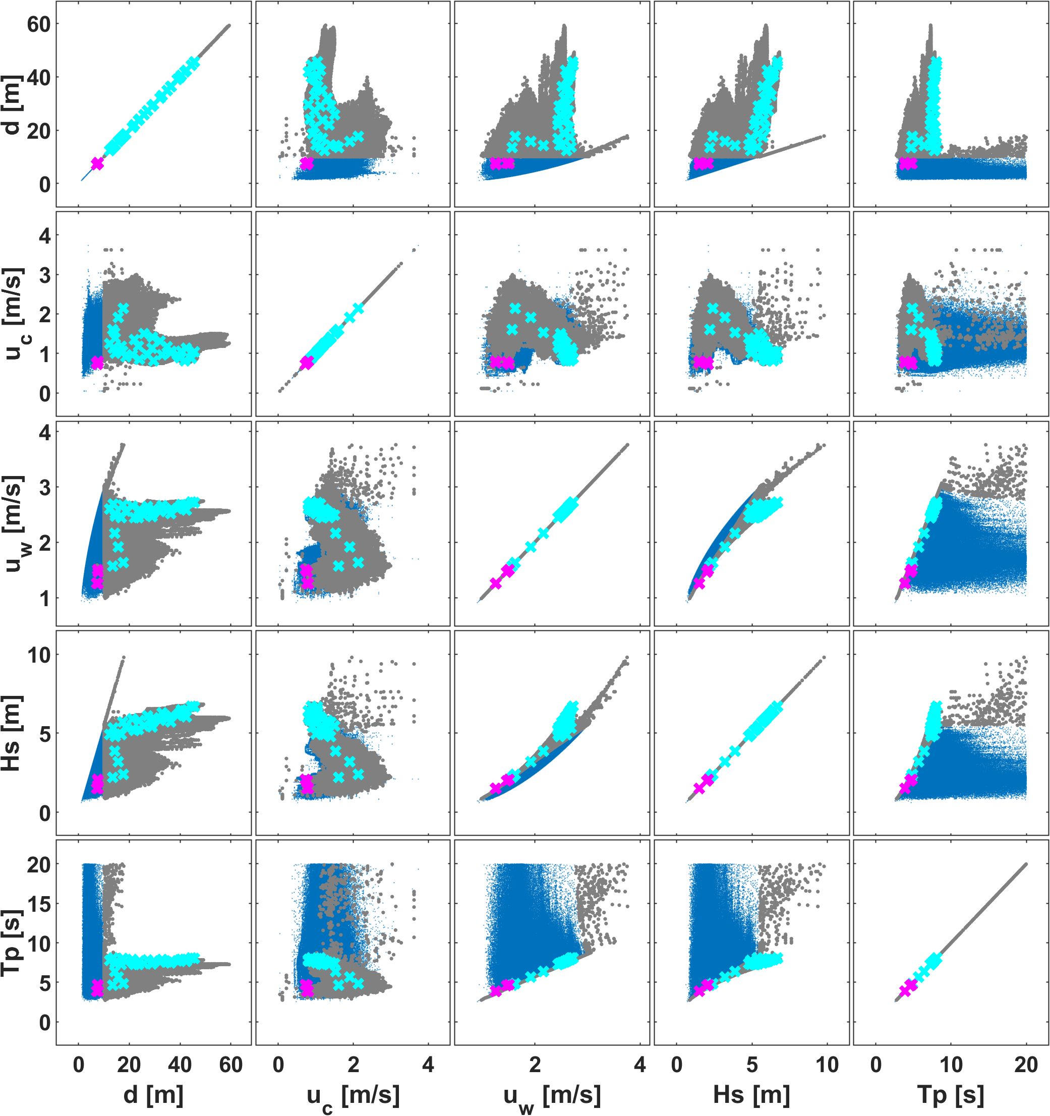
Figure 2. Cluster centroids of the 36 sites (cyan and magenta crosses denote phase one and two of site selection described in Section 2.3) that represent a wide range of water depths and metocean parameters in the German Bight. Blue and grey points denote the full German Bight dataset and the subset from which samples were selected.

Figure 3

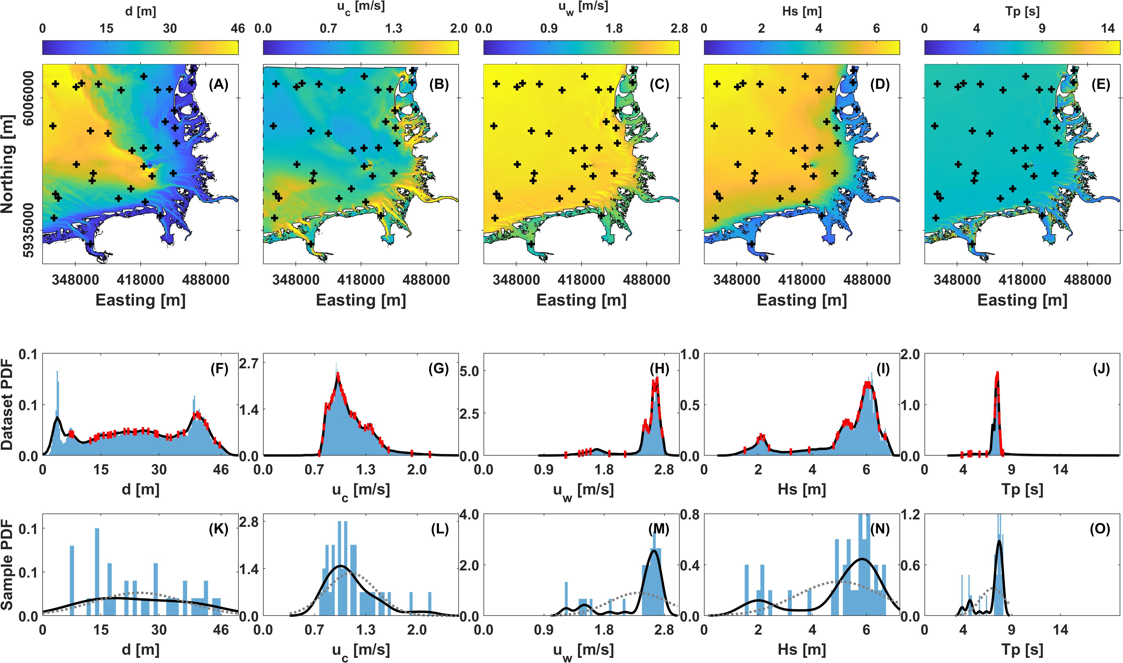
Figure 3. The German Bight in relation to the nearest $x\in C$ to each of the 36 selected sites black crosses in (A–E). From left to right, columns represent the variables: mean depth, 50-year horizontal surface current speed, 50-year horizontal wave orbital velocity amplitude at surface, 50-year significant wave height, and peak wave period associated with 50-year significant wave heights. In (F–J), the selected sites are represented in relation to the histogram and kerel density estimate (KDE) of the PDF by the red vertical points. In (K–O), the histogram and KDE of the sample of 36 selected sites is visualized similarly in comparison to the best fit-fit normal distribution.

2.4 Aquaculture structure design and engineering

The design and engineering of finfish, macroalgae, and shellfish cultivation structures incorporated existing industry and government engineering standards. Several industry and government engineering standards exist, some specific to aquaculture, including: Floating aquaculture farms--Site survey, design, execution and use (NS9415) (Standards Norway, 2022), “A Technical Standard for Scottish Finfish Aquaculture” (Ministerial Group for Sustainable Aquacultures Scottish Technical Standard Steering Group, 2015), “Guidance Notes on the Application of Fiber Rope for Offshore Mooring” (ABS, 2011), “Design and analysis of station keeping systems for floating structures” (API, 2005), and Basis-of-design technical guidance for offshore aquaculture installations in the gulf of Mexico (Fredriksson and Beck-Stimpert, 2019).

NS9415 and the Scottish standard mandate that structures be designed to withstand 50-year storms. No agreed-upon standard exists for non-finfish aquaculture. For uniformity, the 50-year storm condition was used as the design standard for the present study.

For each site selected in Section 2.3, the following procedure was followed: (1) design of cultivation structure with a site-specific mooring design, (2) simulation of cultivation structure under dynamic 50-year conditions (the 50-year storm) based on extreme values of hydrodynamic parameters found in Section 2.2.2, and (3) quantification of the required loading capacities of mooring lines and anchors under 50-year conditions.

2.4.1 Numerical modeling approach

The hypothetical farms are located in exposed ocean sites subject to waves and currents. Each cultivation system is comprised of flexible components subject to nonlinear wave and current forces. Therefore, static analysis of the structure was not sufficient for determining the required structural capacity. Instead, numerical models of the proposed backbone systems were developed using a Hydro-/Structural Dynamic Finite Element Analysis (HS-DFEA) approach. This HS-DFEA approach solves the equations of motion at each time step using a nonlinear Lagrangian method to accommodate the large displacements of structural elements, as described in Fredriksson and Beck-Stimpert (2019) and as applied previously in Coleman et al. (2022) and Moscicki et al. (2024a). Wave and current loading on buoy and line elements (including mussel rope elements) is incorporated into the model using a Morison equation formulation (Morison et al., 1950) modified to include relative motion between the structural element and the surrounding fluid. For elements intersecting the free surface, buoyancy, drag, and added mass forces are multiplied by the fraction of the elements volume that is submerged.

2.4.2 Mussel farm design

The mussel farm consists of a single 200-meter-long backbone line with anchor lines on either end (Figures 4, 5). Mussels are grown on hanging growlines attached to the backbone line, with large floats at anchor line connection points and dropper floats spaced along the backbone line. The structural and hydrodynamic parameters of the mussel lines were taken from Dewhurst (2016) and Dewhurst et al. (2019). The diameter of the mussel ropes was set so that the dry weight of mussels was 12 kg per m of mussel rope. This was based on observations of typical maximum growth on mussel farms in the Gulf of Maine. The net in-water weight of the mature mussel ropes was taken to be ¼ of the dry weight (Bonardelli et al., 2019). Since each backbone in the array has its own anchors and is independent of the other backbones, an individual backbone system was examined with components as defined in Table 1.

Figure 4

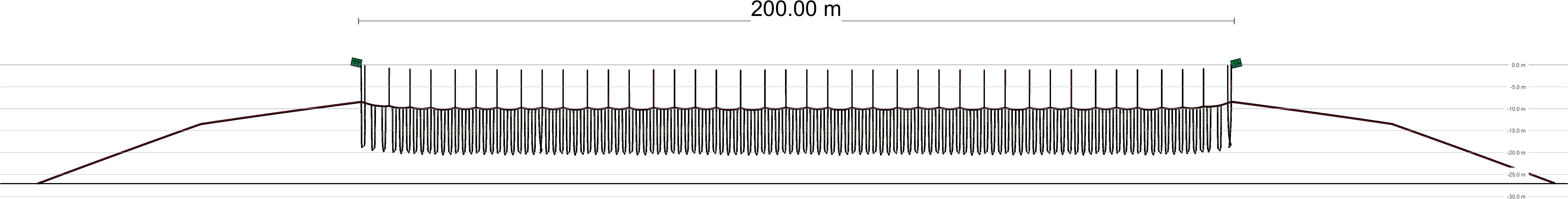
Figure 4. Dimensioned profile view of evaluated backbone system in still water.

Figure 5

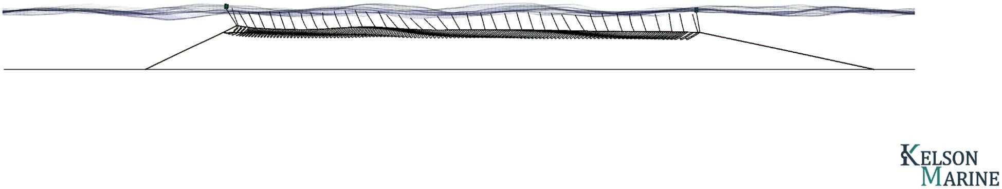
Figure 5. Dynamic HS-DFEA simulation of the mussel backbone system in 50-year storm conditions at Site 27.

Table 1

Table 1. Mussel backbone components as analyzed in HS-DFEA simulations.

2.4.3 Macroalgae farm design

For macroalgae, a tensioned array with 18 growlines (i.e. substrate for macroalgae growth) and four mooring lines was evaluated (Figures 6, 7) The structural layout was similar to that described in (Coleman et al., 2022) but designed to have approximately the same amount of biomass as on the mussel backbone system. The farm is anchored with lines at each corner. A pair of header lines connect the anchor lines and serve as end attachments for the growlines. As with the mussel farm, large buoys are located at each header-anchor line junction and dropper floats are spaced along growlines to maintain buoyancy. Loads on the structure were evaluated using a methodology as described in Moscicki et al. (2024) and validated against the dataset in Fredriksson et al. (2023).

Figure 6

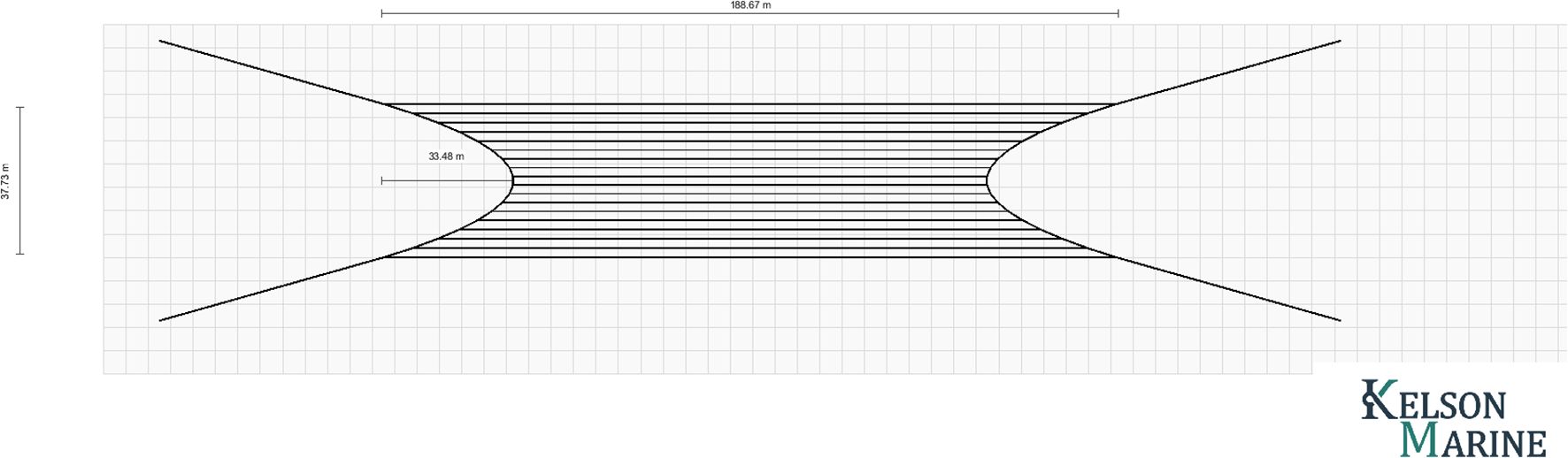
Figure 6. Plan view diagram of the macroalgae cultivation system evaluated.

Figure 7

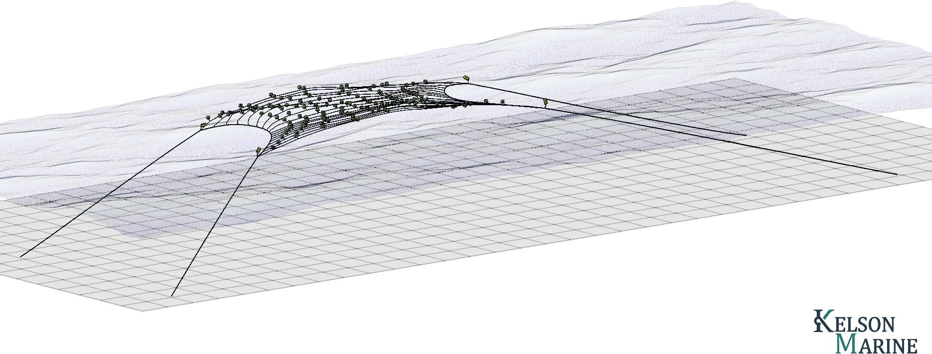
Figure 7. Dynamic HS-DFEA simulation of the macroalgae cultivation system in 50-year storm conditions at Site 18.

2.4.4 Finfish farm design

The finfish structure considered was a single net pen whose properties were based off a prototype built and tested by Gansel et al. (2018). The structure properties as evaluated are given in Table 2. The net hydrodynamics were simulated using a method developed and validated by Kelson Marine that accounts for net solidity, instantaneous relative fluid speed, and incident flow angle on the net panels. This model was validated to within 25% RMS error of the full-scale field measurements reported by Gansel et al. (2018). In the present study, this cage system was embedded in a single-bay, four-mooring line mooring grid as shown in Figures 8, 9.

Table 2

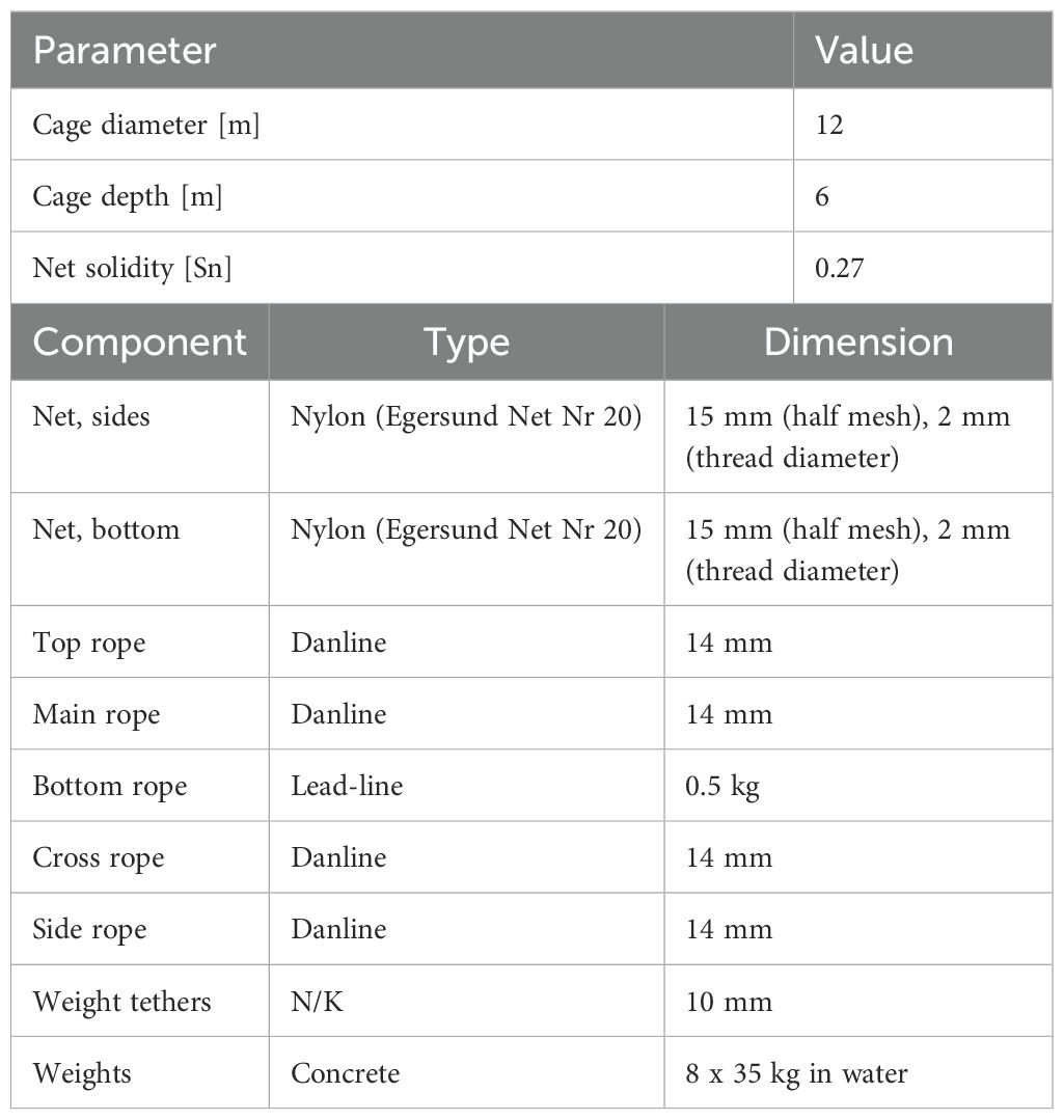
Table 2. Parameters of finfish net pen system evaluated.

Figure 8

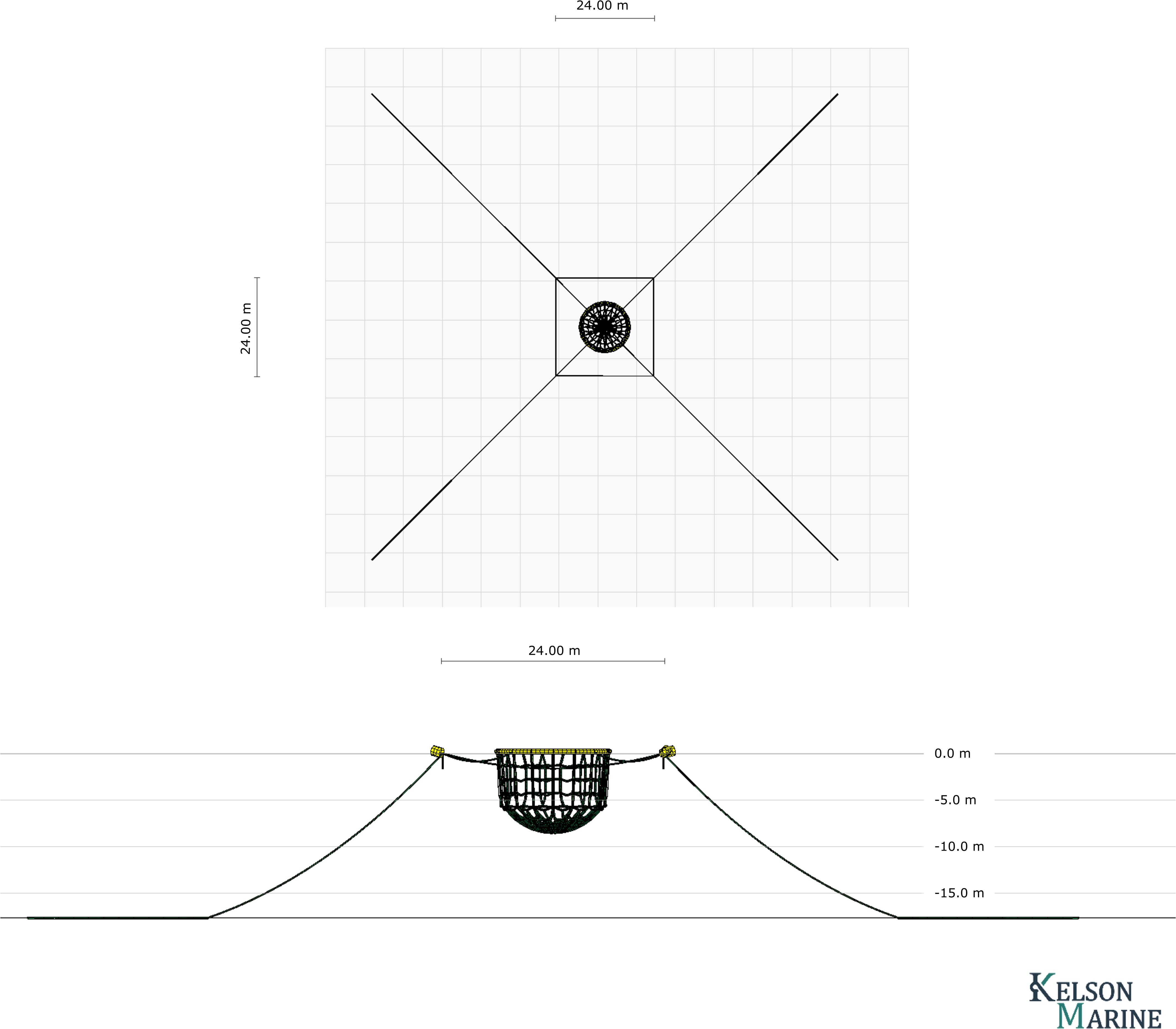
Figure 8. Finfish net-pen and mooring layout considered, showing the design in plan view and in profile view.

Figure 9

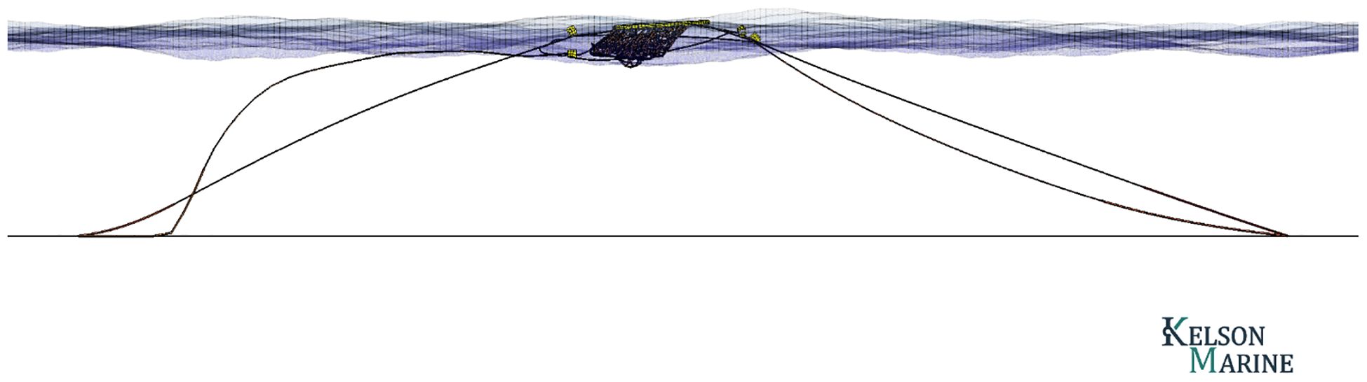
Figure 9. Dynamic HS-DFEA simulation of the finfish net-pen in 50-year storm conditions at Site 19.

2.4.5 Load cases considered

NS 9415 and the Scottish finfish standard mandate that structures be designed to withstand 50-year storms. They stipulate that two 50-year events should be examined in each of the eight compass directional sectors: (1) 50-year wave conditions combined with 10-year current conditions (the wave-dominated case) and (2) 50-year current conditions combined with 10-year wave conditions (the current-dominated case). For simplicity, the present study considered coincident in time and co-directional 50-year wave and 50-year current conditions with no wind loading. Since the seabed is planar and the aquaculture structures are symmetric about at least one axis, three 50-year load cases are evaluated for each farm design, with waves and currents directed at 0, 45, and 90 degree angles relative to their axis of symmetry.

2.4.6 Calculation of required structural capacities

The maximum design loads on all anchoring lines were evaluated based on the results of the dynamic simulations of the cultivation systems at maximum biomass in the 50-year storm conditions. Each of the three farms was simulated for either 900 seconds (finfish) or 1800 seconds (seaweed and shellfish) at each representative site and with three incident wave/current directions. The expected 1-hour extreme loads were calculated from these results using a Peaks-Over-Threshold statistical approach (Coles, 2001). The maximum design load at each representative site is reported as a normalized required capacity (NRC), or

$\begin{array}{ll}\text{NRC}=T/T_{\text{max}}& (7)\end{array}$

where T is the maximum 1-hour extreme loads from each load case at the site and T_max is the maximum load over all sites and load cases.

2.5 Calculation of exposure indices

Exposure indices were computed for each selected aquaculture site. Calculations employed the regional data products described in Section 2.2.2 and 2.2.3 using the mean depths, design hydrodynamic variables defined by the 50-year return values, structure solidity S = 0.25, and structure characteristic length/diameter D = 1.0 m. The $z$ coordinate for the evaluation of the current velocity and wave-induced horizontal orbital velocity amplitudes was set based on the aquaculture structure geometry (see Section 2.4.2, 2.4.3, 2.4.4). The finfish system $z$ coordinate was set halfway down the net-pen to $z = -3$ m, the shellfish $z$ coordinate was set to be the backbone depth and the macroalgae $z$ coordinate was set to a constant depth of the growline or $z = -2$ m. An example map showing the SEE at the surface evaluated over the German Bight is provided in Figure 1. For maps of the full list of proposed indices, see Lojek et al. (2024).

2.6 Linear regression: exploring linear predictors of required structural capacities

The efficacy of exposure indices as a single metric that is approximately proportional to loads on aquaculture structures was evaluated through simple linear regression. Simple linear regression considered the relationships between site specific exposure indices or hydrodynamic variables (i.e. the independent variable or predictor) and sampled normalized required capacities (i.e. the dependent variable or response) (Montgomery et al., 2012; The MathWorks, 2024). Each combination of independent variable $x=\left\{x_1, x_2, \dots ,x_n\right\}$ and dependent variable $y=\left\{y_1,y_2, \dots , y_n\right\}$ was fit to the linear model,

$\begin{array}{ll}y={\beta }_0+{\beta }_{1}x+ϵ& (8)\end{array}$

for model coefficients ${\beta }_0$ and ${\beta }_1$ through minimizing sum of squared residuals in $ϵ=\left\{{ϵ}_1, {ϵ}_2,\dots ,{ϵ}_n\right\}$ . This assumes: (1) a linear $x-y$ relationship, (2) homoscedasticity or equal variance of residuals, (3) normality of residuals, (4) independence of residuals, and (5) absence of outliers. To assess the quality of each regression, results were visualized, the coefficient of determination $R^2$ was calculated to assess the proportion of variance in NRC that is explained by the linear regression with $x$, and bootstrapped confidence interval estimates of regression coefficients and of the line of best fit were calculated. Nonparametric bootstrapping utilized percentile interval confidence intervals at a 0.05 significance level through case resampling (n=1000) to avoid breaking assumptions (3)–(5) (Fox, 2002). Assessment of the normality of the residuals was facilitated by the Anderson-Darling test at a 0.05 significance level (Stephens, 1974; Trujillo-Ortiz, 2007).

3 Results

3.1 Site selection: hydrodynamic parameters and normalized required capacities

Selected mean depths and 50-year hydrodynamic parameters that define representative sites within the German Bight span a range of depths, surface current speeds, and wave environments. These values and the resultant normalized required capacity for each aquaculture structure are reported in Table 3. To place the sites in context from the perspectives of farm operations and to decouple the ideas of “offshore” and “exposed”, the representative distance to coast of the site is reported as well. Normalized required capacities are not reported for sites where the minimum depth exceeds the characteristic length of the aquaculture structure in the z-dimension.

Table 3

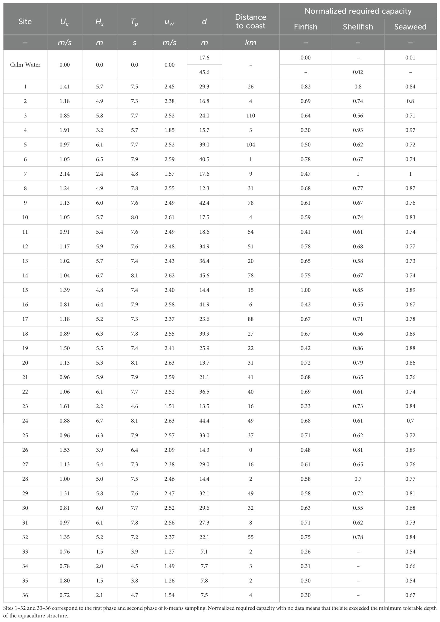
Table 3. Site hydrodynamic parameters and aquaculture structure normalized required capacity.

Figure 3 visualizes the representative selected sites with respect to the German Bight, including normalized histograms and kernel density estimates of the probability distribution functions of the German Bight dataset and representative sites.

Across sites 1–36, depth and hydrodynamic parameter sample distributions are further described by sample means, standard deviations, and measures of skewness. Mean seabed depths across sites range from 7.05 to 45.64 m with a sample mean, standard deviation and skewness of 24.73 m, 11.73 m, and 0.21. Significant wave heights across sites range from 1.5 to 6.7 m with a sample mean, standard deviation and skewness of 5.0 m, 1.6 m and −1.2. The associated peak wave periods range from 3.8 to 8.1 s with a sample mean, standard deviation and skewness of 7.0 s, 0.4 s and −1.3. Wave-induced horizontal wave orbital velocity amplitudes—which depend on depth, significant wave height, and peak wave period—range from 1.26 to 2.63 m/s with a sample mean, standard deviation and skewness of 2.39 m/s, 0.42 m/s and −1.4. Surface current speeds range from 0.72 to 2.14 m/s across sites, with a sample mean, standard deviation and skewness of 1.28 m/s, 0.32 m/s, 1.3. The distance to coastline of representative sites extend from the nearshore to offshore settings, ranging from 0.1 to 110.4 km with a sample mean of 31.1 km, standard deviation of 30.4 km, and positive sample skewness of 1.1.

Across sites 1–32, surface current speeds generally increase with decreasing significant wave heights while the greatest surface current speeds occur at sites with a depth less than 20 m. The associated peak wave periods align with the wave steepness limit.

3.2 Linear regression results: assessing linear predictors of required structural capacities

Linear regression of individual combinations of finfish, shellfish, and seaweed NRCs against $H_s$, $d$, distance to coast, EV, EVRD, SEE, DEF, SDE, and SDBR yielded varying results (Table 4; Figures 10, 11). Presentation of linear regression results are grouped based on linear predictors; results in Section 3.2.1 cover $H_s$, $d$, and distance to coast and Section 3.2.2 cover EV, EVRD, SEE, DEF, SDE, and SDBR. The quality of best-fit regression coefficients ${\beta }_0$ and ${\beta }_1$ in Table 4 is qualitatively assessed by their lower and upper confidence interval estimates. The 95% confidence interval estimates for ${\beta }_0$ and ${\beta }_1$ indicate the uncertainty and the significance of coefficients to the linear regression model. Generally, linear regressions fail to satisfy the assumptions of the homoscedasticity (not shown) and normality of residuals (Table 4 p-values of the Anderson-Darling test for the normality residuals).

Table 4

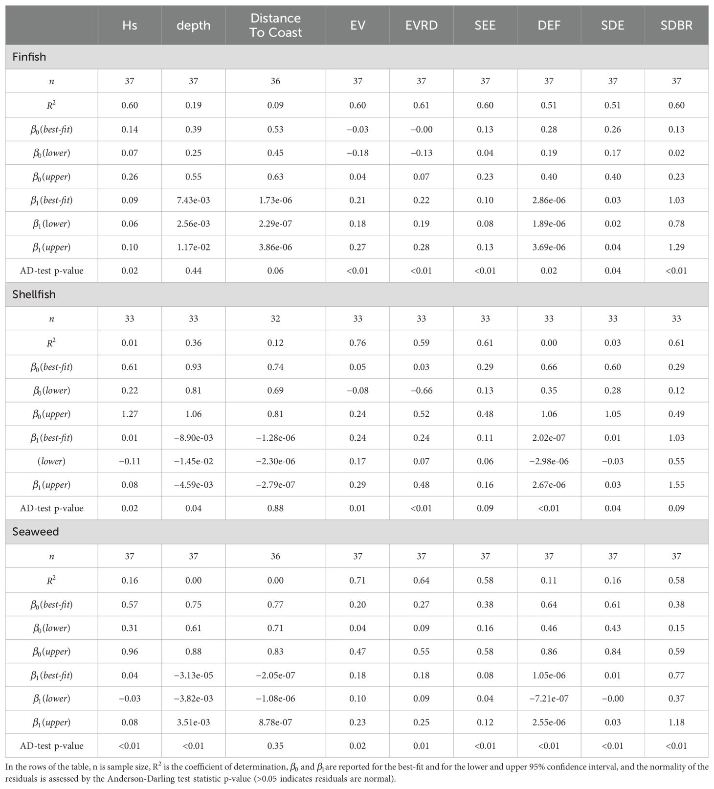
Table 4. Linear regression coefficients and associated statistics for finfish, shellfish, and seaweed structures NRCs for each independent variable considered.

Figure 10

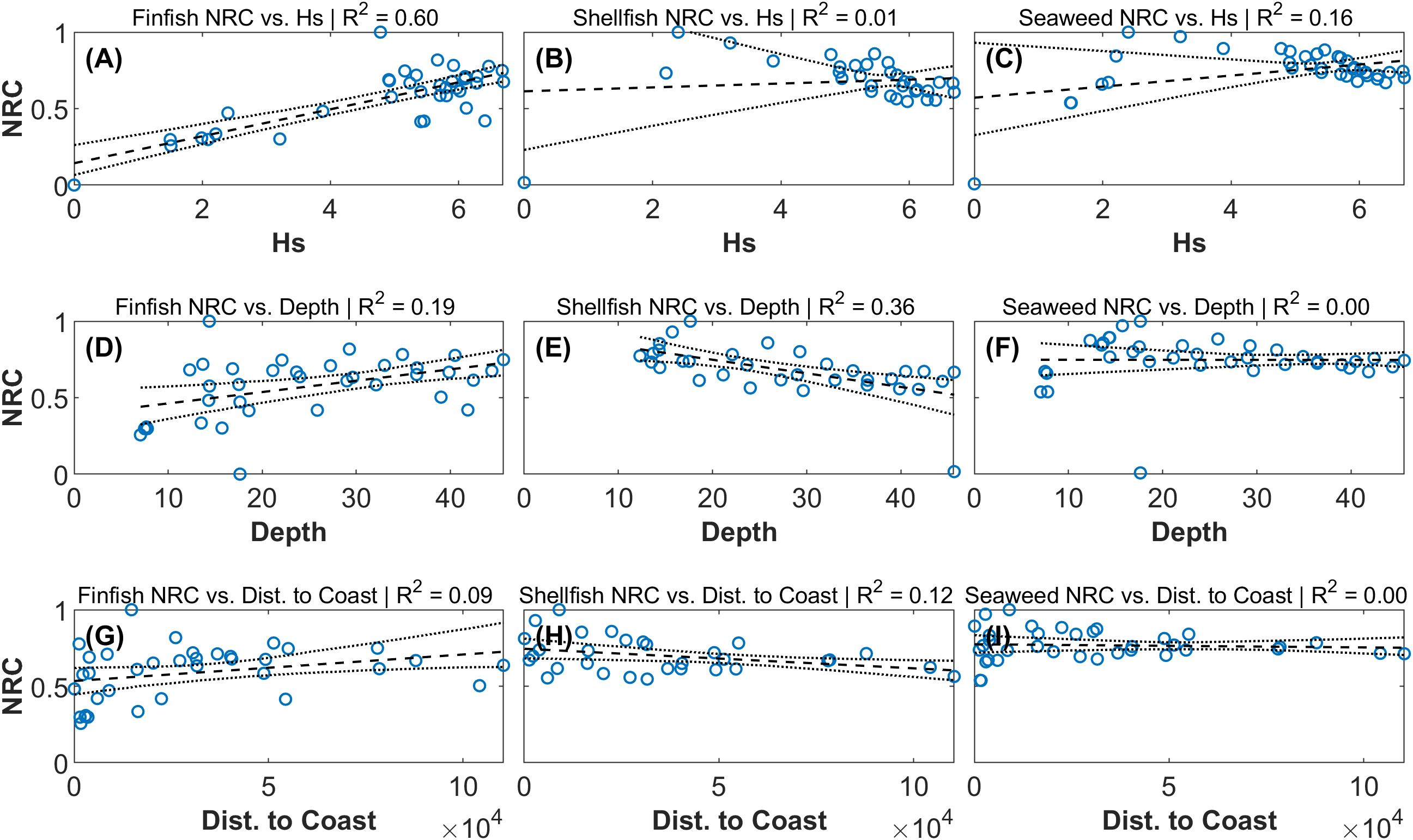
Figure 10. Linear regression of NRC against significant wave height $H_s$ , depth $d$ , and distance to coast; in (A–I) the samples are blue circles, the line of best fit is the dashed black line, and the bootstrapped 95% confidence interval estimates are the dotted black lines. Results are grouped as: (A–C) NRC against Hs in m, (D–F) NRC against d in m, and (G–I) NRC against distance to coast in m.

Figure 11

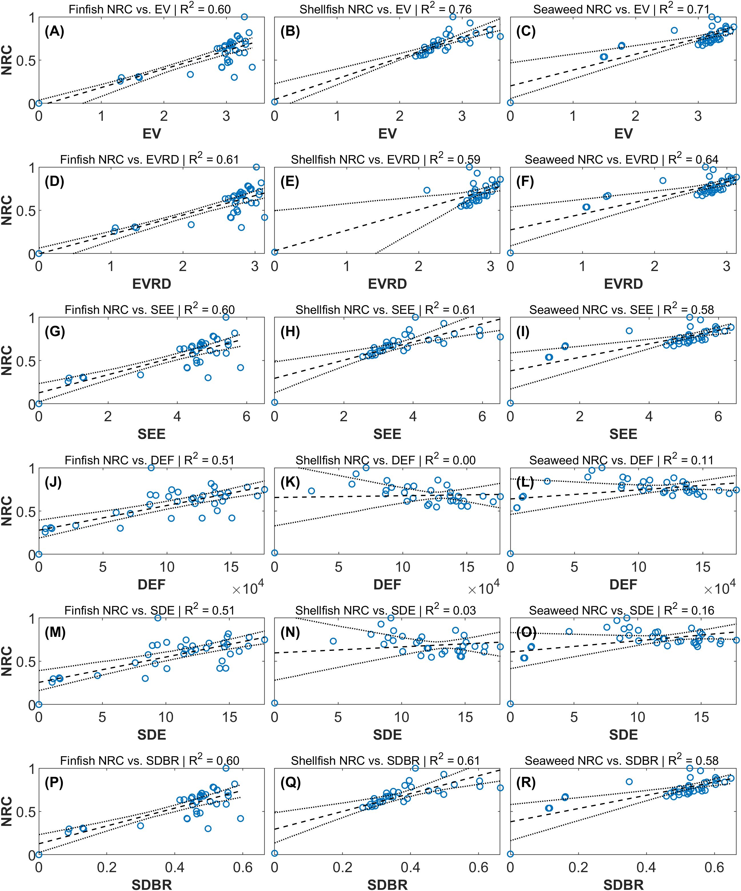
Figure 11. Linear regression of NRC against exposure indices; in (A–R) the samples are blue circles, the line of best fit is the dashed black line, and the bootstrapped 95% confidence interval estimates are the dotted black lines. Results are grouped as NRC against: (A–C) Exposure Velocity $EV$ in m/s, (D–F), Exposure Velocity at a Reference Depth $EVRD$ in m/s, (G–I) Specific Exposure Energy $SEE$ in J/kg, (J–L) Depth-integrated Energy Flux $DEF$ in W/m, (M–O) Structure-centered Depth-integrated Energy $SDE$ J kg/m³, (P–R) Structure-centered Drag-to-Buoyancy Ratio $SDBR$ (non-dimensional).

3.2.1 Significant wave height, depth, and distance to coast as NRC linear predictors

Overall, across the sample sites and structure designs considered, $H_s$, $d$, and distance to coast were not found to be linear predictors of NRC. The relationship between $H_s$ and finfish NRC was the one exception, with the line of best fit explaining up to 60% of the variance. The $R^2$ of remaining relationships was poor, ranging from 0.00 to 0.36 (Figures 10B–I). Near-zero values of ${\beta }_1$ indicates that there is not a linear relationship between $x$ and NRC—as shown in Figures 10B, C, F, G, H, I). Further, confidence intervals of ${\beta }_1$ that cross 0 indicates both uncertainty about the nature of the relationship between $x$ and NRC and that the linear model does not describe the relationship between variables adequately. This pattern is present in linear regression results for shellfish NRC against $H_s$ and seaweed NRC against $H_s$ and $d$. Within the region of German Bight considered, $H_s$, $d$, and distance to coast were not found to be good linear predictors of the finfish, shellfish, and seaweed structures NRC.

3.2.2 Exposure indices as NRC linear predictors

The linear relationships between proposed exposure index and the NRC of finfish, shellfish, and seaweed cultivation structures are shown in Figure 11. Linear regression of NRC against EV, EVRD, SEE, and SDBR explained the greatest proportion of the variance. Across structure types, mean $R^2$ values were 0.69 for EV, 0.61 for EVRD, 0.60 for SEE and SDBR, 0.23 for SDE, and 0.21 for DEF. While all best-fit relationships yielded positive ${\beta }_1$ values, there exists uncertainty about the true values of ${\beta }_1$ as ranges in confidence intervals are of similar magnitudes as the best-fit values. Linear regression of shellfish and seaweed NRC against DEF was not found to generate a suitable model, as noted by the low $R^2$ values and ${\beta }_1$ estimates alternating sign within the 95% confidence interval. Similarly, there is uncertainty surrounding ${\beta }_0$ estimates, with a suggested lack of significance for regressions of finfish NRC against EV and EVRD and shellfish NRC against EV and EVRD. Visual assessment of residuals (not shown) and the p-values of the Anderson-Darling test for the normality of residuals indicate that the linear regression did not satisfy the assumptions of residual homoscedasticity and normality. Bootstrapped 95% confidence intervals for the line of best fit show considerable uncertainty, with greater ranges associated with lower values of the predictor.

4 Discussion

One purpose of an exposure index is to provide a single metric that is approximately proportional to maximum loads on an aquaculture structure. Thus, the efficacy of such an index depends on its positive linear relation to maximum loads on a structure. While structural and operational costs would be more indicative of the relative implications of selecting one site over another, in the absence of a comprehensive costing analysis, the required structural capacity is a reasonable proxy for relative capital expenditure for aquaculture structures. Often mooring line loads are the highest-loaded structural members of a farm. Because component costs are generally proportional to their load capacity, and installation costs are related to the size of the component, the relative structural costs are approximated by mooring line loads.

Previous attempts to define the challenges of “offshore aquaculture” or site exposure have relied heavily on water depth, significant wave height, and distance from the coast (Ryan, 2004; Lovatelli et al., 2013; Froehlich et al., 2017). While these factors may be more influential with respect to operation and maintenance challenges, these metrics were found to be poor predictors of the structural requirements for aquaculture cultivation structures (Figure 10). Required structural capacity and significant wave height demonstrated a linear relationship for finfish structures, yet the same relationship did not exist for shellfish or seaweed structures. Within the region of the German Bight considered, the required structural capacity was found to be negatively related to water depth for shellfish structures, weakly positively related for finfish structures, and independent of depth for seaweed structures. This is because (1) ocean currents are often higher near estuary outlets and nearshore constrictions due to tidal hydrodynamics, and (2) when wind waves with large heights and long wavelengths enter shallow water depths, the resulting horizontal wave-induced particle velocities increase, creating large loads on the cultivation structures considered. The wave shoaling process is captured by the linear relationship between significant wave heights and the required capacities on finfish structures. No similar relation was found for shellfish or seaweed structures, which may be related to the shorter peak wave periods associated with smaller 50-year significant wave heights as defined by the wave steepness limits used in this analysis (DNV, 2010). In regions of the world where extreme wave environments are better characterized by longer peak wave periods, a different relationship may exist. Future work is needed to better define the relationship between the wave environment and structural requirements for aquaculture cultivation structures. Likewise, Depth-integrated Energy Flux (DEF) and Structure-centered Depth-integrated Energy (SDE) were not found to be good predictors of structural requirements and the resulting capital expenditure.

The Exposure Velocity (EV), Exposure Velocity at Reference Depth (EVRD), Specific Exposure Energy (SEE), and Structure-centered Drag-to-Buoyancy Ratio (SDBR) were found to predict design loads on aquaculture structures through a positive linear relationship. Of the sample sites considered in the German Bight, linear models based on EV, EVRD, SEE, or SDBR explained 58% to 76% of the variance in NRC, whereas the classical definitions of offshore sites (greater depths, significant wave heights, and distances to coast) explained 0% to 36% of the variance (with the exception of finfish NRC against $H_s$ which explained 60%). All four of these indices are proportional to the combined wave and current fluid velocities or the square of velocity. The EV was the best predictor of required structural capacity in general, though the uncertainty associated with model coefficients still needs improvement (Table 4). The EV performed better than EVRD since the EV was evaluated at a structure-dependent position in the water column whereas the EVRD was evaluated at the constant reference depth of 5 m. Conversely, depth and distance to coast served as poor predictors for structural load in an easily interpretable way.

The linear relationships between all independent variables and shellfish, finfish, and seaweed structure NRCs reflect the nature of the extreme hydrodynamic conditions of the German Bight. Lower values of the independent variables, such as $H_s$ samples less than 4 m or EV samples less than 2 m/s, implicitly carry more weight in the linear regression. However, all variables considered exist over a continuum; in other seas or coastal ocean regions of the world, extreme values of hydrodynamic variables and their associated exposure indices exist within the lower ranges omitted from this analysis. Further exploration across this full parameter space would better characterize the nature of relationships with NRCs, either through a systematic study of synthetic but feasible site conditions or through repeating this analysis procedure across dynamically different regions of the coastal ocean.

Again—the basis of the exposure indices is such that it should provide a positive linear indication of exposure. In this context, a negative linear relationship is clearly undesirable, as is a non-linear relationship. Hence, the linear regression used for evaluation and the favoring of results that best characterize positive linear relationships. Though more work is needed to more accurately characterize the nature of the relationship of exposure indices with design loads on aquaculture structures, this study provides evidence that the EV, EVRD, SEE, and SDBR can support or improve site suitability assessment methods.

Inherent assumptions of the HS-DFEA analysis method could bias agreement towards certain variables or indices over others. Assumptions about hydrodynamic interaction with the structure and the physics incorporated in these models may be better replicated by some indices. While the aquaculture systems chosen for this analysis were selected based on their representative qualities, the specific design choices inherent to these systems may bias the results of this study. Substantial differences in system characteristics, such as mooring line axial stiffness, can result in significantly different loading in the same environmental conditions. The computational resources required to simulate a wide variety of system designs for all sites and load cases were prohibitive in the context of this study. Further, exposure indices do not account for loads related to system inertia in the dynamic scenarios. Due to these nuances and specific design choices, use of exposure indices to estimate structural load does not replace a true engineering study.

5 Conclusion

The Exposure Velocity (EV), Exposure Velocity at Reference Depth (EVRD), Specific Exposure Energy (SEE), and Structure-centered Drag-to-Buoyancy Ratio (SDBR) can provide a coarse estimate of the required capacity of an aquaculture structure across a range of sites. These exposure indices yielded the strongest performance as a positive linear predictor of the normalized required capacities of finfish, shellfish, and macroalgae aquaculture structures at potential sites within the German Bight of the North Sea, with $R^2$ values of 0.69, 0.61, 0.60, and 0.60 for EV, EVRD, SEE, and SDBR, respectively. Though none of the linear relationships exhibit adequate precision to be used as the basis for engineering design or detailed cost estimation, the findings suggest that EV, EVRD, SEE, and SDBR and other proposed indices based on fluid speed hold significantly more meaning than depth, distance from shore, or significant wave height when communicating about a site's exposure between developers, regulators, investors, insurers, farmers, and technology providers. Structural loads and costs are only a part of the larger siting process; these factors are often misinterpreted or completely left out of the decision-making framework due to the practical barrier of a comprehensive engineering evaluation of all potential sites and structure designs of interest. Though they do not replace a true engineering study, these indices can be generated quickly from widely available public data to inform siting, risk assessment, and relative costs of aquaculture structures.

Data availability statement

The original contributions presented in the study are included in the article/supplementary material. Further inquiries can be directed to the corresponding author.

Author contributions

TD: Conceptualization, Data curation, Formal analysis, Funding acquisition, Investigation, Methodology, Project administration, Resources, Software, Supervision, Validation, Visualization, Writing – original draft, Writing – review & editing. SR: Data curation, Formal analysis, Investigation, Methodology, Visualization, Writing – original draft, Writing – review & editing. MM: Data curation, Formal analysis, Investigation, Methodology, Software, Validation, Visualization, Writing – original draft, Writing – review & editing. NB: Formal analysis, Software, Validation, Visualization, Writing – original draft, Writing – review & editing. ZM: Formal analysis, Investigation, Software, Validation, Visualization, Writing – original draft, Writing – review & editing.

Funding

The author(s) declare financial support was received for the research, authorship, and/or publication of this article. The authors thank Innovasea Systems Inc. for funding the publishing fee for this article.

Conflict of interest

The authors declare that the research was conducted in the absence of any commercial or financial relationships that could be construed as a potential conflict of interest.

Publisher’s note

All claims expressed in this article are solely those of the authors and do not necessarily represent those of their affiliated organizations, or those of the publisher, the editors and the reviewers. Any product that may be evaluated in this article, or claim that may be made by its manufacturer, is not guaranteed or endorsed by the publisher.

References

ABS (2011). Guidance Notes on the Application of Fiber Rope for Offshore Mooring. August 2011 (Updated March 2012) (Houston, TX: American Bureau of Shipping).

Google Scholar

API R. (2005). Design and analysis of station keeping systems for floating structures (Washington, D.C.: American Petroleum Institute, API Publishing Services).

Google Scholar

Bonardelli J. C., Kokaine L., Ozolina Z., Aigars J. (2019). Technical evaluation of submerged mussel farms in the Baltic sea Kurzeme planning region Kalmar municipality. SUBMARINER Network, Berlin, Germany. Available Online at: https://2020.submariner-network.eu/images/BBG_submerged_V1.pdf.

Google Scholar

Browdy C. L., Hargreaves J. A. eds. (2009). Overcoming Technical Barriers to the Sustainable Development of Competitive Marine Aquaculture in the United States. U.S. Department of Commerce, Silver Spring, MD USA: NOAA Technical Memo NMFS F/SPO100. 114pp.

Google Scholar

Buck B. (2007). Farming in a high energy environment : potentials and constriants of sustainable offshore aquaculture in the German Bight (North Sea). Bremerhaven, Germany: Alfred Wegener Institute - Reports on Polar and Marine Research. Available Online at: https://core.ac.uk/download/pdf/11769689.pdf.

Google Scholar

Buck B. H., Krause G., Michler-Cieluch T., Brenner M., Buchholz C. M., Busch J. A., et al. (2008). Meeting the quest for spatial efficiency: progress and prospects of extensive aquaculture within offshore wind farms. Helgoland Mar. Res. 62 (3), 269–281. doi: 10.1007/s10152-008-0115-x

Crossref Full Text | Google Scholar

Buck B. H., Troell M. F., Krause G., Angel D. L., Grote B., Chopin T. (2018). State of the art and challenges for offshore integrated multi-trophic aquaculture (IMTA). Front. Mar. Sci. 5. doi: 10.3389/fmars.2018.00165

Crossref Full Text | Google Scholar

Buck B. H., Bjelland H. V, Bockus A., Chambers M., Costa-Pierce B. A., Dewhurst T., et al. (2024). Resolving the term “offshore aquaculture” by decoupling “exposed” and “distance from the coast”. Front. Aquaculture 3. doi: 10.3389/faquc.2024.1428056

Crossref Full Text | Google Scholar

Buck B., Langan R. (2017). Aquaculture perspective of multi-use sites in the open ocean: the untapped potential for marine resources in the anthropocene, aquaculture perspective of multi-use sites in the open ocean: the untapped potential for marine resources in the anthropocene. Cham, Switzerland: Springer Nature. doi: 10.1007/978-3-319-51159-7

Crossref Full Text | Google Scholar

Byrne M. (2011). Impact of ocean warming and ocean acidication on marine invertebrate life history stages: Vulnerabilities and potential for persistence in a changing ocean, in Oceanography and Marine Biology. 1st edn (Boca Raton: CRC Press), 1–42. Available Online at: https://www.taylorfrancis.com/books/edit/10.1201/b11009/oceanography-marine-biology-gibson-atkinson-gordon?refId=a7aae774-a9b1-4cd1-8619-843791ea5d0c&context=ubx.

Google Scholar

Clawson G., Kuempel C. D., Frazier M., Blasco G., Cottrell R. S., Froehlich H. E., et al. (2022). Mapping the spatial distribution of global mariculture production. Aquaculture 553, 738066. doi: 10.1016/j.aquaculture.2022.738066

Crossref Full Text | Google Scholar

Coleman S., Dewhurst T., Fredriksson D. W., St. Gelais A. T., Cole K. L., MacNicoll M., et al. (2022). Quantifying baseline costs and cataloging potential optimization strategies for kelp aquaculture carbon dioxide removal. Front. Mar. Sci. 9. doi: 10.3389/fmars.2022.966304

Crossref Full Text | Google Scholar

Coles S. (2001). An introduction to statistical modeling of extreme values (Springer-Verlag London: Springer).

Google Scholar

Dewhurst T. (2016). Dynamics of a submersible mussel raft. PhD dissertation (Durham, New Hampshire: University of New Hampshire).

Google Scholar

Dewhurst T., Hallowell S. T., Newell C. (2019). “Dynamics of an array of submersible mussel rafts in waves and current,” in Proceedings of the international conference on offshore mechanics and arctic engineering - OMAE. Glasgow, Scotland, UK: American Society of Mechanical Engineers. doi: 10.1115/OMAE2019-96388

Crossref Full Text | Google Scholar

DNV (2010). Environmental conditions and environmental loads, Dnv. Oslo, Norway: DNV or Det Norske Veritas. doi: 10.1109/INTLEC.1993.388591

Crossref Full Text | Google Scholar

Duarte C. M., Holmer M., Olsen Y., Soto D., Marbà N., Guiu J., et al. (2009). Will the oceans help feed humanity. BioScience 59, 967–976. doi: 10.1525/bio.2009.59.11.8

Crossref Full Text | Google Scholar

Falconer L., Hunter D.-C., Scott P.C., Telfer T., Ross L. (2013). Using physical environmental parameters and cage engineering design within GIS-based site suitability models for marine aquaculture. Aquaculture Environ. Interact. 4, 223–237. doi: 10.3354/aei00084

Crossref Full Text | Google Scholar

FAO, IFAD, UNICEF, WFP, WHO. (2020). “The state of food security and nutrition in the world 2020,” in Transforming food systems for affordable healthy diets(Rome: FAO). doi: 10.4060/ca9692en

Crossref Full Text | Google Scholar

Fox J. (2002). Bootstrapping regression models, appendix to an R and S-PLUS companion to applied regression. Available online at: https://artowen.su.domains/courses/305a/FoxOnBootingRegInR.pdf (Accessed 23 October 2024).

Google Scholar

Fredriksson D. W., Beck-Stimpert J. (2019). Basis-of-design technical guidance for offshore aquaculture installations in the gulf of Mexico, Vol. 2019. U.S. Department of Commerce, Silver Spring, MD USA. doi: 10.25923/r496-e668

Crossref Full Text | Google Scholar

Fredriksson D. W., St. Gelais A. T., Dewhurst T., Coleman S., Brady D. C., Costa-Pierce B. A. (2023). Mooring tension assessment of a single line kelp farm with quantified biomass, waves, and currents. Front. Mar. Sci. 10. doi: 10.3389/fmars.2023.1178548

Crossref Full Text | Google Scholar

Froehlich H. E., Smith A., Gentry R. R., Halpern B. S. (2017). Offshore aquaculture: I know it when I see it. Front. Mar. Sci. 4. doi: 10.3389/fmars.2017.00154

Crossref Full Text | Google Scholar

Gansel L. C., Oppedal F., Birkevold J., Tuene S. A. (2018). Drag forces and deformation of aquaculture cages—Full-scale towing tests in the field. Aquacultural Eng. 81, 46–56. doi: 10.1016/j.aquaeng.2018.02.001

Crossref Full Text | Google Scholar

Gephart J. A., Pace M. L., DOdorico P. (2014). Freshwater savings from marine protein consumption. Environ. Res. Lett. 9, 14005. doi: 10.1088/1748-9326/9/1/014005

Crossref Full Text | Google Scholar

Gimpel A., Stelzenmüller V., Grote B., Buck B. H., Floeter J., Núñez-Riboni I., et al. (2015). A GIS modelling framework to evaluate marine spatial planning scenarios: Co-location of offshore wind farms and aquaculture in the German EEZ. Mar. Policy 55, 102–115. doi: 10.1016/j.marpol.2015.01.012

Crossref Full Text | Google Scholar

Goseberg N., Chambers M., Haesmann K., Fredriksson D., Fredheim A., Schlurmann T. (2017). Technological approaches to longline- and cage-based aquaculture in open ocean environments. Cham, Switzerland: Springer Nature, 71–95. doi: 10.1007/978-3-319-51159-7_3

Crossref Full Text | Google Scholar

Hagen R., Plüß A., Freund J., Ihde R., Kösters F., Schrage N., et al. (2020). EasyGSH-DB: themengebiet - hydrodynamik [Data set]. Karlsruhe, Germany: Bundesanstalt für Wasserbau (BAW). doi: 10.48437/02.2020.K2.7000.0003

Crossref Full Text | Google Scholar

Hagen R., Plüß A., Ihde R., Freund J., Dreier N., Nehlsen E., et al. (2021). An integrated marine data collection for the German Bight – Part 2: Tides, salinity, and waves, (1996–2015). Earth System Sci. Data 13, 2573–2594. doi: 10.5194/essd-13-2573-2021

Crossref Full Text | Google Scholar

Hannemann O. (2024). OpenSeaMap version 0.1.23. Available online at: https://map.openseamap.org/ (Accessed 19 August 2024)).

Google Scholar

Hartigan J. A., Wong M. A. (1979). Algorithm AS 136: A K-means clustering algorithm, journal of the royal statistical society. Ser. C (Applied Statistics) 28, 100–108. doi: 10.2307/2346830

Crossref Full Text | Google Scholar

Hilborn R., Hilborn U. (2012). Overfishing: what everyone needs to know (New York, NY: Oxford University Press).

Google Scholar

Klein H., Frohse A. (2008). Oceanographic processes in the german bight. In: Die Küste 74. Heide, Holstein: Boyens. S., 60–76. Available at: https://henry.baw.de/items/7c47dc78-47e1-44e8-aea3-38202ee4d5d0 (Accessed September 1, 2024).

Google Scholar

Limburg K. E., Waldman J. R. (2009). Dramatic declines in north atlantic diadromous fishes. BioScience 59, 955–965. doi: 10.1525/bio.2009.59.11.7

Crossref Full Text | Google Scholar

Lojek O., Goseberg N., Føre H. M., Dewhurst T., Bölker T., Haesman K. G., et al. (2024). Hydrodynamic exposure -On the quest to deriving quantitative metrics for mariculture sites. Front. Aquaculture. 3. doi: 10.3389/faquc.2024.1388280

Crossref Full Text | Google Scholar

Lovatelli A., Aguilar-Manjarrez J., Soto D. (2013). Expanding mariculture farther offshore: Technical, environmental, spatial and governance challenges (Orbetello, Italy). Available online at: https://www.fao.org/4/i3092e/i3092e.pdf (Accessed 23 October 2024).

Google Scholar

Marra J. (2005). When will we tame the oceans. Nature 436, 175–176. doi: 10.1038/436175a

PubMed Abstract | Crossref Full Text | Google Scholar

Ministerial Group for Sustainable Aquacultures Scottish Technical Standard Steering Group (2015). A technical standard for scottish finfish aquaculture. Available online at: https://www.gov.scot/binaries/content/documents/govscot/publications/advice-and-guidance/2015/06/technical-standard-scottish-finfish-aquaculture/documents/00479005-pdf/00479005-pdf/govscot%3Adocument (Accessed May 5, 2024).

Google Scholar

Montgomery D., Peck E., Vining G. (2012). Introduction to linear regression analysis. 5th edn (Hoboken, New Jersey: John Wiley & Sons).

Google Scholar

Morison J. R., Johnson J. W., Schaaf S. A. (1950). The force exerted by surface waves on piles. J. Petroleum Technol. 2, 149–154. doi: 10.2118/950149-G

Crossref Full Text | Google Scholar

Moscicki Z., Swift M. R., Dewhurst T., MacNicoll M., Chambers M., Tsukrov I., et al. (2024). Design, deployment, and operation of an experimental offshore seaweed cultivation structure. Aquacultural Eng. 105, 102413. doi: 10.1016/j.aquaeng.2024.102413

Crossref Full Text | Google Scholar

Moscicki Z., Swift M. R., Dewhurst T., MacNicoll M., Fredriksson D. W., Chambers M., et al. (2024a). Evaluation of an experimental kelp farms structural behavior using regression modelling and response amplitude operators derived from in situ measurements. Ocean Eng. 305, 117877. doi: 10.1016/j.oceaneng.2024.117877

Crossref Full Text | Google Scholar

Nijdam D., Rood T., Westhoek H. (2012). The price of protein: Review of land use and carbon footprints from life cycle assessments of animal food products and their substitutes. Food Policy 37, 760–770. doi: 10.1016/j.foodpol.2012.08.002

Crossref Full Text | Google Scholar

NOAA (2016). Fisheries of the caribbean, gulf, and south atlantic; aquaculture; final rule. Federal Register 81 (8), 1765–1787. Available Online at: https://www.govinfo.gov/content/pkg/FR-2016-01-13/pdf/2016-00147.pdf.

Google Scholar

NOAA (2017). Understanding fisheries management in the United States. Available online at: https://www.fisheries.noaa.gov/insight/understanding-fisheries-management-united-states (Accessed 19 August 2024).

Google Scholar

Oremus K. L. (2019). Climate variability reduces employment in New England fisheries. PNAS 116, 26444–26449. doi: 10.1073/pnas.1820154116

PubMed Abstract | Crossref Full Text | Google Scholar

Pawlowicz R. (2020). M_Map: A mapping package for MATLAB version 1.4m, [Computer software]. Available online at www.eoas.ubc.ca/~rich/map.html.

Google Scholar

Porporato E. M. D., Pastres R., Brigolin D. (2020). Site suitability for finfish marine aquaculture in the central mediterranean sea. Front. Mar. Sci. 6. doi: 10.3389/fmars.2019.00772

Crossref Full Text | Google Scholar

Przedrzymirska J., Zaucha J., Calado H., Lukic I., Bocci M., Ramieri E., et al. (2021). Multi-use of the sea as a sustainable development instrument in five EU sea basins, sustainability, Basel, Switzerland: MDPI Sustainability. Vol. 13 (15). doi: 10.3390/su13158159

Crossref Full Text | Google Scholar

Puniwai N., Canale L., Haws M., Potemra J., Lepczyk C., Gray S. (2014). Development of a GIS-based tool for aquaculture siting. ISPRS Int. J. Geo-Information 3, 800–816. doi: 10.3390/ijgi3020800

Crossref Full Text | Google Scholar

Rosenthal H., Hilge V. (2000). Aquaculture production and environmental regulations in Germany. J. Appl. Ichthyology 16, 163–166. doi: 10.1046/j.1439-0426.2000.00272.x

Crossref Full Text | Google Scholar

Ryan J. (2004). Farming the deep blue. Available online at: https://bim.ie/wp-content/uploads/2021/02/Farming,the,Deep,Blue.pdf (Accessed 23 October 2024).

Google Scholar

Sanchez-Jerez P., Karakassis I., Massa F., Fezzardi D., Aguilar-Manjarrez J., Soto D., et al. (2016). Aquacultures struggle for space: the need for coastal spatial planning and the potential benefits of Allocated Zones for Aquaculture (AZAs) to avoid conflict and promote sustainability. Aquaculture Environ. Interact. 8, 41–54. doi: 10.3354/aei00161

Crossref Full Text | Google Scholar

Sievers J., Karakassis I., Massa F., Fezzardi D., Aguilar-Manjarrez J., Soto D., et al. (2021). An integrated marine data collection for the German Bight – Part 1: Subaqueous geomorphology and surface sedimentolog 2016). Earth System Sci. Data 13, 4053–4065. doi: 10.5194/essd-13-4053-2021

Crossref Full Text | Google Scholar

Sievers J., Rubel M., Milbradt P. (2020). “EasyGSH-DB: bathymetrie,” in Bundesanstalt für wasserbau. Karlsruhe, Germany: Bundesanstalt für Wasserbau (BAW). doi: 10.48437/02.2020.K2.7000.0002

Crossref Full Text | Google Scholar

Standards Norway (2022). NS 9415:2021 (en) Floating aquaculture farms Site survey, design, execution and use. Oslo, Norway: Standards Norway (Standard Norge).

Google Scholar

Stephens M. A. (1974). EDF statistics for goodness of fit and some comparisons. J. Am. Stat. Assoc. 69, 730–737. doi: 10.2307/2286009

Crossref Full Text | Google Scholar

The MathWorks I. (2024). Linear regression. Available online at: https://www.mathworks.com/help/matlab/data_analysis/linear-regression.html (Accessed October 2024).

Google Scholar

Theuerkauf S. J., Barrett L. T., Alleway H. K., Costa-Pierce B. A., St. Gelais A., Jones R. C. (2022). Habitat value of bivalve shellfish and seaweed aquaculture for fish and invertebrates: Pathways, synthesis and next steps. Rev. Aquaculture 14, 54–72. doi: 10.1111/raq.12584

Crossref Full Text | Google Scholar

Troell M., Metian M., Beveridge M., Verdegem M., Deutsch L. (2014). Comment on “Water footprint of marine protein consumption—aquacultures link to agriculture. Environ. Res. Lett. 9, 109001. doi: 10.1088/1748-9326/9/10/109001

Crossref Full Text | Google Scholar

Trujillo-Ortiz A. (2007). AnDartest. MATLAB central file exchange. Available online at: https://www.mathworks.com/matlabcentral/fileexchange/14807-andartest (Accessed 23 October 2024).

Google Scholar

Wessel P., Smith W. H. F. (1996). A global, self-consistent, hierarchical, high-resolution shoreline database. J. Geophysical Research: Solid Earth 101, 8741–8743. doi: 10.1029/96JB00104

Crossref Full Text | Google Scholar