From lithological descriptions to geological models: an example from the Upper Aare Valley

Introduction: Geological models provide a critical foundation for hydrogeological models and significantly influence the spatial distribution of key hydraulic parameters such as hydraulic conductivity, transmissivity, or porosity. The conventional modeling workflow involves a hierarchical approach that simulates three levels: stratigraphical units, lithologies, and finally properties. Although lithological descriptions are often available in the data (boreholes), the same is not true for unit descriptions, leading to potential inconsistencies in the modeling process.

Methodology: To address this challenge, a geostatistical learning approach is presented, which aims to predict stratigraphical units at boreholes where this information is lacking, primarily using lithological logs as input. Various standard machine learning algorithms have been compared and evaluated to identify the most effective ones. The outputs of these algorithms are then processed and utilized to simulate the stratigraphy in boreholes using a sequential approach. Subsequently, these boreholes contribute to the construction of stochastic geological models, which are then compared with models generated without the inclusion of these supplementary boreholes.

Results: This method is useful for reducing uncertainty at certain locations and for mitigating inconsistencies between units and lithologies.

Conclusion: This approach maximizes the use of available data and contributes to more robust hydrogeological models.

1 Introduction

The foundation of groundwater models is largely based on conceptual models and derived geological models, as they constrain most of the key parameters such as hydraulic conductivity (K), boundary conditions, and layer geometries [1]. Typically, the established approach involves delineating the geometry of major stratigraphical units (unit model), populating these units with facies (or lithologies) using suitable facies modeling methods, and subsequently assigning physical properties to the facies (property model). Note here that the concept of stratigraphical units is considered in its strict sense, which means that the units are differentiated by their age, not by their lithologies that they contain or their sedimentological setting. Although these information often provide important information that helps in their definition and identification. Throughout these steps, various data sources, including borehole and geophysical data, play a pivotal role. This workflow, widely adopted in the geosciences for decades [2–5], is due to its robustness, flexibility, and ability to replicate diverse geological contexts effectively.

One major drawback of this approach is that it generally involves different algorithms and softwares due to the large complexity of the problem, this is particularly true for Quaternary formations which are still difficult to model today, despite a rich geological modeling history (e.g. [3, 6, 7]).

To address these issues, Schorpp et al. [5] recently introduced ArchPy, a semi-automated hierarchical approach. ArchPy operates across the three aforementioned levels (units, facies, and properties), with a specific capability to consider unit hierarchies. This concept, common in sedimentology, involves smaller subunits contained within larger units, a feature generally lacking in other modeling software. Additionally, ArchPy can reach any level of unit hierarchy, the only limitation is the geological concept and the interpreted data that need to be consistent with it. At the core of the ArchPy approach lies the use of the Stratigraphic Pile (SP), serving as a container for all expert knowledge pertinent to a specific geological problem. The SP encompasses not only the different units for simulation and the corresponding facies, but also all algorithms and associated parameters for modeling these geological entities. Once the SP is defined, subsequent modeling processes, including data processing, simulations, and validation, become streamlined and predominantly automated. The philosophy is to shift the focus of modelers toward conceptualizing the SP, emphasizing the geological concept, and minimizing the manual effort required for data processing. Furthermore, ArchPy allows one to generate stochastic simulations, a critical capability for tasks such as uncertainty quantification and inverse modeling. The successful application of ArchPy in these contexts, combined with geophysical data, has been demonstrated in recent studies [8, 9].

However, a significant challenge with ArchPy, like many geostatistical methods, is the requirement for a significant amount of geological data, primarily obtained from boreholes, to generate accurate and reliable models. Boreholes can provide information regarding units (stratigraphic log), facies (lithological log), and/or properties (e.g. pump test values). Although lithological logs are commonly easier to obtain, determining stratigraphic units is a harder task, often resulting in the absence of stratigraphic logs. The issue here is that, as units and facies steps are simulated separately (but not independently), inconsistencies can arise.

Even though there may be no simple relationship between units and lithologies, the definition of stratigraphic units often adheres to a logic that tends to separate geological time periods with different climatic and sedimentological settings, resulting in the deposition of different types of sediments [10]. As a consequence, some units can be mainly composed of coarse sediments (gravels, sand) or, conversely, fine sediments (clay, silt). In cases where stratigraphic logs are missing, simulations may yield inconsistent facies models compared to unit models, as illustrated in Figure 1. In this simple example, the absence of the unit log for borehole B2 leads to an inaccurate representation of the interface between A and B. Subsequently, the simulated facies will be partially erroneous, and a portion of the facies log for B2 will not be respected. Note that while this is a simplified illustration, determining the true unit log is not challenging in this case. In reality, more complex relations emerge, where dozens of units and facies can be combined.

Figure 1

Figure 1. Illustrative example demonstrating a possible consequence of the absence of the unit log. Borehole B2 is excluded from the simulation of the surface (green line), leading to inconsistent results. The surface must pass at the interface between unit B and A, corresponding to the interface between the facies clay, silt vs. gravel, sand (indicated by the asterisk).

Recently, machine learning (ML) algorithms have emerged as an interesting alternative to traditional methods for dealing with spatial data in various applications (e.g. [11–16]). In particular, one can cite Rigol et al. [11] who have used an artificial neural network as an interpolator for temperature data with very good prediction results, comparable to standard geostatistical techniques such as kriging. Several authors have studied and reported the differences between parametric and nonparametric methods when applied to spatial data (e.g. [14, 15, 17, 18]). All these comparative studies have shown that ML algorithms can deliver similar or even superior results to geostatistical methods. It is interesting to note, however, that methods such as random forests often show superior predictive qualities in terms of confidence intervals and hence uncertainty [18]. However, such results must be viewed with caution, as they are highly dependent on the situation, the sampling strategy, the amount of data, etc.

There have also been attempts to use machine learning to predict geology. For example, Aliouane et al. [19] evaluated the performance of various ML algorithms for the prediction of lithology. Similarly, Hammond and Allen [20] employed Artificial Neural Networks in conjunction with Self-Organizing Maps to predict the spatial distribution of lithofacies in a large and intricate glacial aquifer, using a substantial database of more than 13,000 boreholes. Another notable example is the work of Sahoo and Jha [21], who applied a similar approach on a smaller scale, achieving highly accurate prediction results with precisions reaching 90%. Furthermore, Zhou et al. [22] suggested the application of a recurrent neural network, a form of Deep Learning network, to directly model sequences of geological units (i.e., boreholes) based on geographical coordinates.

However, it is crucial to note that these methodologies were developed to model specific geological entities (such as units or facies) in isolation, without an explicit consideration of the interdependence between them. Addressing this limitation, Li et al. [23] have introduced a sequential approach in which a stratigraphic ML model is initially trained on spatial coordinates only. Subsequently, the results of this model are used to constrain a facies ML model, ensuring coherence between stratigraphic and facies representations and avoiding the challenges depicted in Figure 1.

To fill this gap, our study introduces a novel approach for inferring stratigraphical units using lithological descriptions and geographical coordinates. This methodology is applied to the Upper Aare Valley. A stochastic geological model is generated and compared with a similar model that integrates these new sources of information. The paper is organized as follows. Section 2 presents the material and methods, consisting of the definition of the problem, an overview of the study area and the available data, the construction of the geological model, and finally the details about the methodology used to infer the stratigraphy. Finally, Sections 5 and 6 present and discuss the results, along with an exploration of potential limitations and opportunities for improvement within the current workflow.

2 Materials and methods

2.1 Problematic

The objective is to predict the stratigraphy at a specific depth in a borehole where it is missing. This is achieved by utilizing a set of input explanatory variables, which consist of the lithology in the borehole at this depth, as well as the lithologies above and below this point, and geographical coordinates.

Mathematically, we define a set of boreholes $B$ and for each borehole $b_i\in B$, we have geographical coordinates g_i = (x_i, y_i), where (x_i, y_i) represents the borehole horizontal position. In addition, each borehole has vertical information about the lithological data l_i (e.g. clay, gravel, sand) and the stratigraphy s_i. These are given at different heights z_j and depths d_j, where the subscript j indicates a particular interval in b_i. Boreholes are separated in two groups, those who have an information about the stratigraphy ${\text{S}}_{\mathrm{\text{known}}}=\left\{{\text{s}}_i\mid b_i\in B_{\mathrm{\text{known}}}\right\}$, where $B_{\mathrm{\text{known}}}\subset B$, and those who do not have the stratigraphy and are defined as the rest of the boreholes $B_{\mathrm{\text{missing}}}=B\backslash B_{\mathrm{\text{known}}}$. The aim here is to predict the stratigraphy s_k for boreholes $b_k\in B_{\mathrm{\text{missing}}}$. This can be viewed as a supervised problem where a set of inputs X_i = (g_i, l_i): combined geographical and lithological features for borehole b_i are used to predict an output y_i = s_i, which corresponds to the stratigraphy for borehole b_i. Given a certain training dataset $D_{\mathrm{\text{train}}}=\left\{({\text{X}}_i,{\text{y}}_i)\mid b_i\in B_{\mathrm{\text{known}}}\right\}$, it is possible to train a function f as shown in Equation 1:

$\begin{array}{ll}f({\text{X}}_i)\approx {\text{y}}_i\text{for }{b}_i\in B_{\text{known}}& (1)\end{array}$

And using f, we can predict the stratigraphy as shown in Equation 2:

$\begin{array}{ll}{\text{s}}_j=f({\text{X}}_j)\text{ for }{b}_j\in B_{\text{missing}}& (2)\end{array}$

The final outputs of this procedure are series of stochastic simulated stratigraphic logs s_k for boreholes $b_k\in B_{\mathrm{\text{missing}}}$ that can eventually be used to constrain geologic models and help maintain consistency between stratigraphy and lithology.

In this paper, we propose to emulate the function f from Equations 1 and 2 with a two-step procedure: first, complex and non-linear relationships between inputs and outputs are learned using ML algorithms, and second, the probabilistic outputs of the ML algorithms are used in a well simulation step to ensure that the generated wells respect the stratigraphy. To test the feasibility of this method, a geological model based on real data was built and used. Finally, two models are compared, one without considering the boreholes $b_k\in B_{\mathrm{\text{missing}}}$ and one with them where the stratigraphy has been predicted. It should be noted that the present method does not necessitate the construction of a geological model for its implementation. Its purpose is to test the efficacy of our methodology and to ascertain the impact of integrating simulated boreholes with our methodology on the final geological models.

Before going into the details of the methodology, the study area, the available data and the construction of the geological model are presented.

2.2 Study area

2.2.1 Geological context

The test area selected for this methodology is the Upper Aare Valley, which is a Quaternary Alpine Valley situated between the cities of Thun and Bern in Switzerland (Figure 2). This valley has undergone a complex geological history primarily influenced by glacial and river processes [24, 25]. The main river in the valley is the Aare, which flows from south to north. Previous investigations focused on Quaternary deposits, regionally [26, 27], as well as locally [28, 29], have revealed complex relationships among various depositional and erosional processes, including fluvial, glacial, glacio-fluvial, and glacio-lacustrine. Consequently, the geology of the valley is diverse and exhibits a wide range of sediments and facies, such as tills/moraines, fluvial gravels, glacio-lacustrine deposits, lake deposits, and alluvial cones, contributing to the notable heterogeneity of these deposits. From a hydrogeological point of view, two primary aquifers have been identified: a shallow aquifer actively utilized for drinking water supply, shallow geothermal energy and local industries, and a deeper aquifer, which remains poorly understood due to its greater depth (with only a limited number of boreholes reaching it). The thickness of the shallow aquifer exhibits variation, ranging from 0 to 5 m in the north, where a local absence of the aquifer can be observed, to 50–80 m in the south.

Figure 2

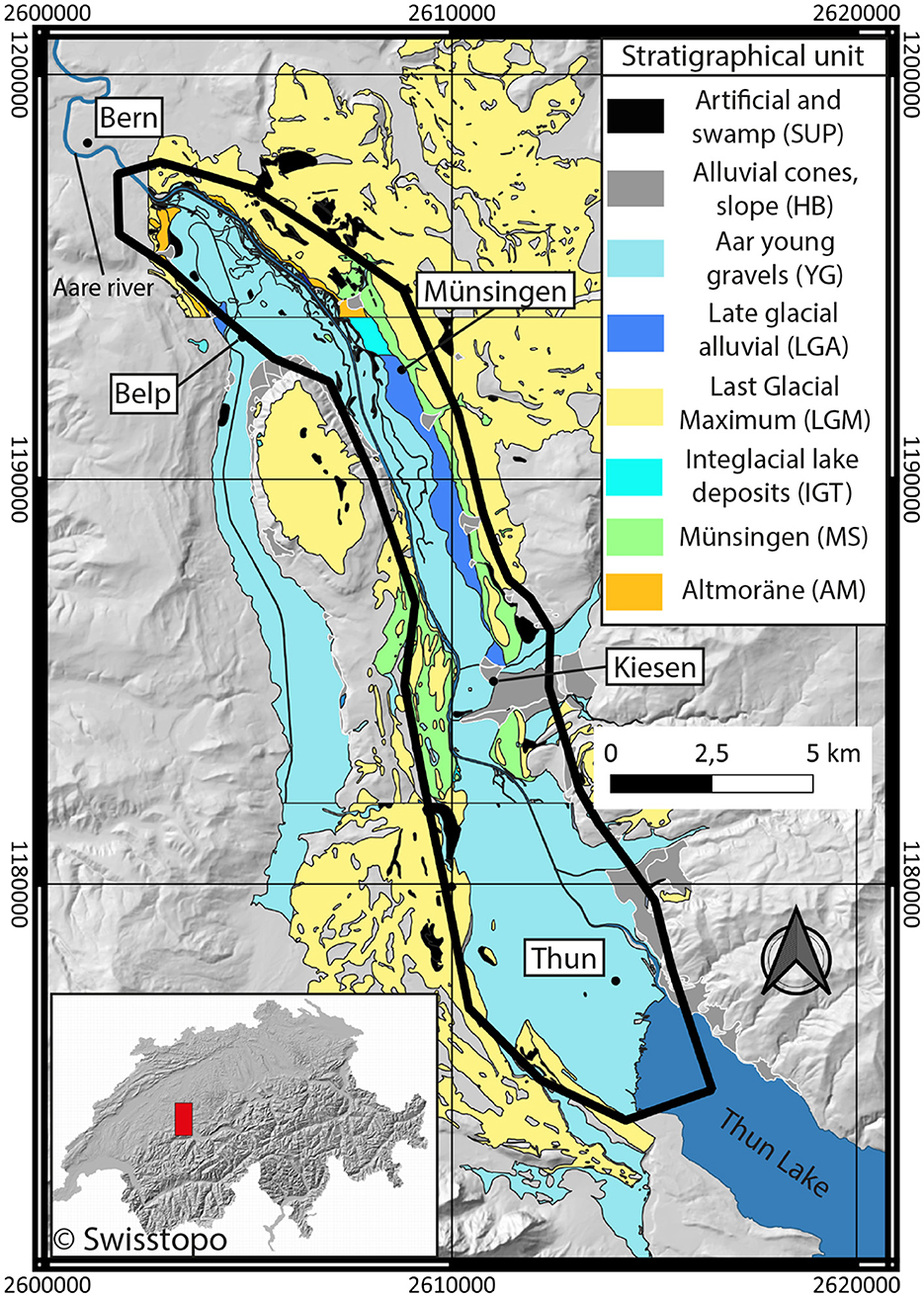
Figure 2. Geographical situation and simplified geological map of the Upper Aare Valley. Only unconsolidated deposits are shown. The coordinates are presented in CH1903+ - LV95 (epsg : 2056). All data used come from the Swiss Geological Survey (Swisstopo) and are freely accessible. The black polygon delimits the modeling area for the study.

A brief summary of the geological history is presented, but a more complete geological review can be found in Kellerhals et al. [24]. It begins in the Pleistocene, where the erosion of the Swiss Molasse (bedrock) by the glaciers has shaped the valleys that can be observed today. The earliest Quaternary sediments, locally denominated as “Alte Seetone” (AT), are old lacustrine deposits that make up the valley's predominant geological volume, presuming the presence of a large lake at that time. Locally, these deposits are overlain by Oppligen sands (OS), a unit mainly composed of sand (>70%), compared to the others. Ascending further, the Uttigen-Bümberg-Steghalde gravels (UBS), a fluvial deposit, rest atop AT and OS. This particular formation is known to be a major constituent of the deep aquifer. AT, OS, and UBS do not outcrop (Figure 2), and are shallower in the southern and lateral parts of the valley. Following these events, one or more glacial episodes were recorded, attributed to the previously named Riss glaciation. These episodes entailed the erosion of existing deposits and the deposition of new ones, specifically glaciolacustrine deposits (GL), “Altmoräne” (AM, Old Moraine, probably from Riss glaciation), and retreat fluviogravels, following a typical glacial sequence. The retreat gravels have practically all been eroded. This sequence is followed by an interglacial lacustrine clay (IGT). Outcrops and borehole observations of GL, AM, and IGT are limited, predominantly located on the northern sides of the valley.

Following the interglacial stage, a major gravel deposition event, Münsingen gravels (MS) can still be found across the whole valley. This occurs right before the last glacial maximum (LGM), during which large moraines have been deposited. After LGM, phases of late glaciation followed, with localized and anecdotal deposits of gravel and moraine. The conclusion of these late glacial phases is marked by post- to late-glacial lacustrine deposits (LGL). In addition to the LGLs, postglacial to lateglacial gravels (LGA) were also deposited. Subsequently, the Aare River contributed to the deposition of gravel (YG), forming a significant component of the upper aquifer. These gravels are occasionally overlain by slope deposits and lateral alluvial fans (HB), as well as swamp and artificial deposits (SUP). LGL, LGA, YG and HB are located in the center of the main and lateral valleys and are surrounded by the bedrock and the other units.

2.2.2 Available data

The Swiss Geological Survey has compiled and standardized a significant borehole database [30], resulting from a substantial data set that comprises 791 boreholes for the designated area. The distribution of the depths of the boreholes is highly uneven. The vast majority (>95%) of the depths of the boreholes range between a few and 50 m deep, while some outliers can reach up to 200 m. Each borehole is characterized by intervals containing information on granulometry (lithologies), stratigraphical units, and details regarding the quality and reliability of the interpretations. The rich geological history has contributed to the identification of many interpreted stratigraphical units (24 in total). However, it should be noted that only one third of the wells includes a unit description (266 out of 791 boreholes, see Figure 3), and certain units are absent within the modeling area. Granulometry information is described with one, two, or up to three distinct grain sizes, each defined following the USCS system [31].

Figure 3

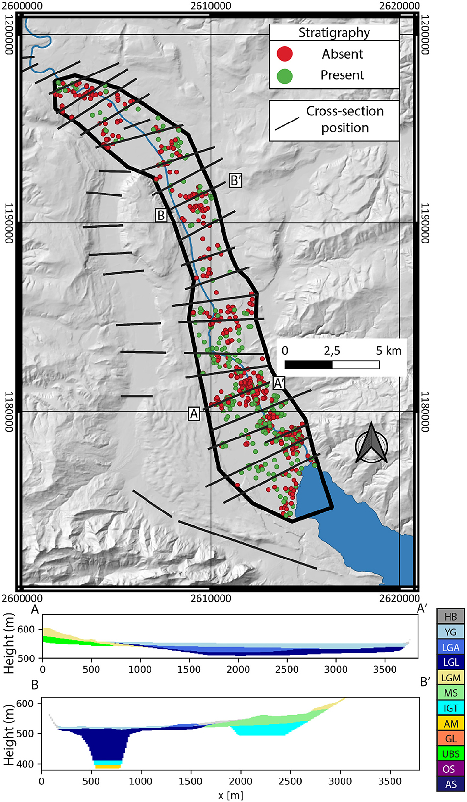
Figure 3. Borehole and cross-section positions over the modeling area. Boreholes with stratigraphic unit descriptions are colored in green while those without are colored in red. Two cross-sections, whose positions are marked by (A–A') and (B–B'), are also shown. The colors used in the cross-sections to represent the units are described in Figure 4.

In addition to boreholes, a set of geological cross sections has been drawn by Kellerhals et al. [24] (Figure 3), complemented by a geological map (Figure 2), derived from the GeoCover dataset of the Swiss Geological Survey. The cross sections do not reach the bottom of the valley and provide limited information about deep geology, but still provide constraints at shallow depths (< 50 m).

2.3 Geological model

Recently, several studies have tested different approaches to model the heterogeneity of the valley [5, 9, 30, 32], supported by recent geophysical data acquisition, nearly over the entire valley [33]. Neven et al. [32] proposed a clay fraction model that combined boreholes and geophysical data in a stochastic workflow. However, a limitation of their approach was the lack of geological consistency in the final model. This issue was addressed to some extent in a subsequent work, where ArchPy was integrated with a joint inversion workflow utilizing an Ensemble Smoother with Multiple Data Assimilation [9]. However, the geological model used in this refinement remained restricted (complete stratigraphy not considered, lacking a facies modeling step), leaving room for further enhancements. In response to these considerations, a comprehensive and stochastic geological model of the Upper Aare Valley is presented, drawing on available geological data.

The model is constructed using the ArchPy geological modeling package [5], which is based on the Geone¹ geostatistical library. ArchPy workflow is hierarchical and relies on three major steps: units, facies (lithologies), and properties. In the unit simulation, 2D surfaces are simulated to delineate the upper and lower boundaries of each unit. Subsequently, facies simulation employs 3D categorical methods (facies methods) to fill the previously simulated units with facies. Finally, independent continuous simulations are performed within each facies to obtain the property models.

2.3.1 ArchPy pile

The main ingredient of an ArchPy model is the definition of the Stratigraphic Pile (SP). The SP does not solely consist in defining the order of deposition of the units but also the interpolation (and related parameters) to use to delimit their lateral extent, the type of contact of their top surface, the lithologies that compose these units, etc. Alternatively, the SP can be viewed as the geological concept translated into a format comprehensible by the modeling package, in this case ArchPy. The SP for the present study is shown in Figure 4.

Figure 4

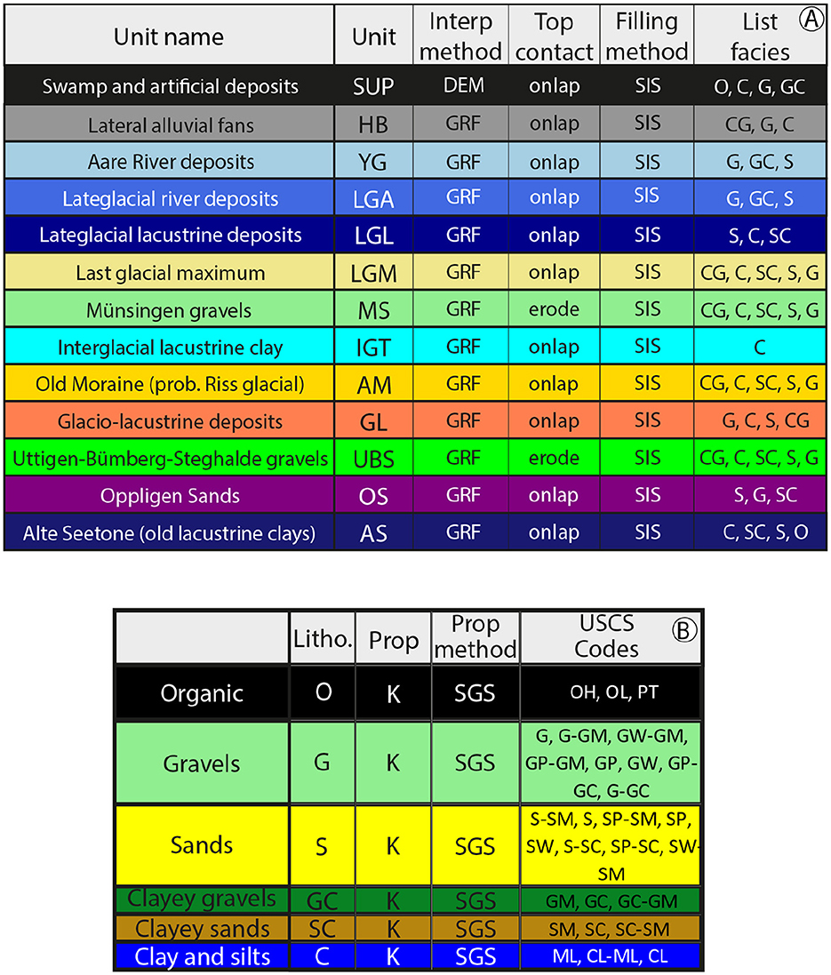
Figure 4. ArchPy Stratigraphic Pile for the Aar model. (A) Details about the stratigraphic unit such as interpolation method (GRF: Gaussian Random Function), contact of top surface, filling method for the facies step and the list of facies to model inside this unit. (B) Facies table containing details about the facies such as the property to simulate (K: hydraulic conductivity), Interpolation method (SGS: Sequential Gaussian Simulation) and USCS codes that correspond to the facies.

Compared to the 24 units identified in the GeoQuat database, 13 have been retained. This reduction mainly results from the absence of certain units in the boreholes, together with considerations for the simplification of the geological concept. The simulation of all unit surfaces (interp method column, Figure 4A) uses Gaussian Random Functions (GRF) [34], except for the SUP unit, where its top surface is simply set at the elevation of the Digital Elevation Model (DEM). Two surfaces, MS and UBS, are treated as erosive. This decision is based on the assumption that, at the conclusion of these units, a significant glaciation event occurred, suggesting a corresponding major erosive episode. To keep things simple, Sequential Indicator Simulation (SIS) [35] is used to model the distribution of the lithology.

Lithologies are categorized into six groups according to the main grain size, expressed in terms of USCS codes. The corresponding codes for each category are provided in Figure 4B. Sequential Gaussian simulation (SGS) [36] is used to simulate the hydraulic conductivity (K), the unique property considered in this study, but others can be easily and quickly integrated.

The assignment of facies to units is determined by their relative proportions (Figure 5). If a facies constitutes < 5%, it is supposed to be absent from the unit. The facies associations for each unit exhibit a degree of similarity, with similar units that showcase analogous facies compositions. For instance, LGM and AM, both moraines, encompass nearly all categories, aligning with the expectation that moraines exhibit very poor sorting. However, we can observe that the aquifer formations (YG, LGA, MS, UBS, and OS) mainly contain the most permeable categories (G, S, and GC). However, MS and UBS also include clay (C) and clayey sand (SC), which shows that the relationship between facies and units is not so straightforward.

Figure 5

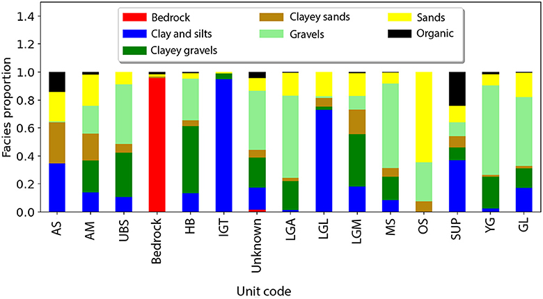
Figure 5. Lithologies group proportions in each of the stratigraphic units. In addition, proportions are also given for the bedrock unit and when the unit is unknown.

2.3.2 Data and modeling grid

Input data are the boreholes described in the previous section as well as the geological map (Figure 2) and the cross sections (Figure 3). To be used with ArchPy and take advantage of its automated processing step, these two data (map and cross-sections) are converted into fake boreholes. In practice, random locations are drawn on the geological map and at each of these locations, a small 10 cm borehole taking the stratigraphy at that location is created. For cross-sections, vertical stratigraphic information is extracted at several locations along the section and converted into ArchPy boreholes. In this way, the 2D array representing the section is transformed into a series of 1D representations (boreholes). The spacing between these boreholes must be small enough to retain the structures present in the section. In our case, a distance of 150 m was chosen.

The extent of the modeling considers the polygon shown in Figure 2, with a spatial resolution set at 25 × 25 × 2 m (sx×sy×sz). The origin of the z direction is established at 350 m above sea level, with the maximum elevation reaching 590 m above sea level. This configuration results in a grid size of 548 × 958 × 120 cells (nx×ny×nz). The top of the domain is defined by the Swiss DEM with a resolution of 25 × 25 m (DHM25, Swisstopo). At the same time, the bottom is determined by a raster map of the elevation of the bedrock (TopFels25, Swisstopo), which also has a resolution of 25 × 25 m. Both datasets are accessible through the Swiss Federal Office of Topography. Only the cells that lay between the top and the bottom surfaces are considered.

2.3.3 Modeling parameters

Once the SP, a grid, and the data are defined, ArchPy processes the boreholes which are analyzed and necessary data extracted. This step automatically determines the equality data (data points through which a surface must pass) and inequality data (data indicating that the surface must go above or below this point) for surface interpolation. The result is a list of coordinates for the equality and inequality data for each unit. More details on this procedure can be found in Schorpp et al. [5].

In order to use GRF, covariance models (variograms) must be specified for each top surface. For YG, LGA, and LGL, where no discernible anisotropy is apparent, isotropic models were automatically fitted (through least-square optimization) to their equality points. However, for the remaining units, a clear anisotropy is observed, aligned with the main axis of the valley. Unfortunately, the number of points is insufficient to estimate a reliable 2D variogram. Consequently, a default anisotropic variogram model was estimated using the elevation surface of the bedrock (TopFels25) as a surrogate, which is known and assumed to represent the general shape of the unit surfaces. The total variance for each unit was adjusted on the basis of the observed variance in the data. Additionally, this model incorporates a locally variable anisotropy through an rotation map that accounts for the orientation of the axis of the valley.

The facies modeling stage using SIS also necessitates variograms, one for each facies within each unit. These variograms were initially automatically fitted and then manually adjusted, assuming that there was no horizontal anisotropy (i.e., the variogram range in the x-direction equals the range in the y-direction) whenever the number of data points was sufficient. It was necessary to perform a manual adjustment to prevent the introduction of inconsistencies, such as variograms with very short ranges, which were likely the result of an inability to identify an optimized variogram. In some cases, the quantity of data was insufficient to permit an appropriate fitting. In such cases, variograms for the same facies in another unit were considered. Visualization of some variograms can be found in Supplementary Figures S4–S9.

For the simulation of hydraulic conductivity (K), no available data were used to estimate the variograms. Instead, they were defined on the basis of previous research in the area [5, 9] and the scientific literature related to similar lithologies [37, 38].

Complete details of the variograms for each unit, facies, and property, as well as the anisotropic map, are shown in Supplementary material.

2.4 Borehole stratigraphy inference

This section outlines the methodology used to predict stratigraphic unit information in boreholes where it is absent, relying on lithological and spatial information. The approach is divided into two distinct steps: first, a machine learning (ML) step where algorithms are trained and applied to derive probabilities of unit occurrences along the boreholes; and second, the utilization of these probabilities in a simulation step to generate plausible boreholes. The data considered for this analysis are boreholes from the GeoQuat database, simplified according to the ArchPy Pile (Figure 4), resulting in 13 units for six lithofacies. Two more classes, not used in the geological model, have been considered in the ML process, which are Bedrock and None. None represents a gap in the unit log interpretation.

2.4.1 Machine learning step

Initially, the boreholes are divided into two datasets, a training set and a test set, for the validation of the present methodology. Of the 791 existing boreholes, only 266 contain stratigraphic information (Figure 3), forming the total data set. From these 266 boreholes, a training set is generated, consisting of 75% (200) of the boreholes, while the test set comprises the remaining 25% (66) of the boreholes. The spatial distribution of the two sets are shown in the Supplementary Figure S1. This partition is achieved through iterative stratified sampling, ensuring a similar unit proportion distribution in both sets. The iterative process has been run until the disparity in class distribution between the two sets was below 2%. It is important to note that some units, such as AM or IGT, are very rare and are present in only a few boreholes. This rarity posed challenges for stratified sampling, resulting in a less straightforward and imperfect process.

To integrate borehole information into the ML process, it is essential to transform training and test sets into data structures consisting of features (inputs) and labels (outputs). ML algorithms, operating on each data point characterized by multiple features, generate predictions for a single label or assign probabilities to each potential label. Obviously, algorithms are trained to give the best possible predictions. Features can take a variety of forms, including continuous or categorical values, but each data point must consistently have the same number of features. Figure 6 illustrates how a training borehole is transformed into a collection of multiple data points, each with its list of features and the resulting labels.

Figure 6

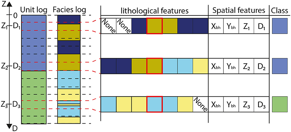
Figure 6. Schematic representation of the features and label creation of training borehole for the machine learning algorithm. For the sake of clarity, only three data are shown, but each interval in the borehole, separated by the dashed lines, is transformed. For each interval i, there is a datum defined by seven categorical lithological features that correspond to the three lithologies above and below the interval, as well as the lithology in the interval (surrounded in red). If no lithology data are available above or below, the feature is set as “none.” Furthermore, four additional numerical features are considered, which are: the x and y coordinates of the borehole (X_bh and Y_bh, respectively), the elevation (Z_i) and depth (D_i) of the interval.

Boreholes are initially segmented into intervals of uniform thickness (e), and for each interval, a data point is constructed using a list of lithological and spatial features that vary along the boreholes. The spatial features consist of four elements: the x, y, and z coordinates of the interval (X_bh, Y_bh, and Z_i), along with its depth relative to the top of the borehole (D_i). Regarding lithological features, they encompass the lithology observed within the interval (red square in Figure 6), as well as a specified number of lithologies above (n_a) and below (n_b). In Figure 6, three intervals are considered above and below (n_a = n_b = 3). If multiple lithologies are observed within a single interval, the most dominant one is considered (see Figure 6).

The inclusion of lithologies both above and below a given interval serves a crucial purpose in mitigating potential errors in predictions arising from the presence of rare or inconsistent lithology/unit associations.To illustrate this, consider a scenario involving an aquifer unit primarily composed of gravel and sands. In the presence of thin sporadic clay layers (with a thickness of e), relying solely on the lithology within the specific interval can lead to inaccuracies in ML predictions, such as incorrectly predicting that these intervals belong to another unit, possibly one that is more clay rich. However, if we integrate a larger picture of the situation by considering the lithologies above and below, this effect can be mitigated.

e, n_a and n_b are user inputs of the methodology that need to be defined. e should be low enough to capture vertical variability in terms of lithologies in the modeling area. On the contrary, n_a and n_b should be high enough to encompass a sufficient number of lithological variations above and below each interval. Conceptually, these parameters act as a viewing window through which the algorithm can gain insight into the prediction problem. For this study, the selected parameters are e = 20 cm, n_a = n_b = 10, indicating the consideration of a 2 m span above and below each interval with a resolution of 20 cm. This roughly corresponds to the finest level of detail that can be obtained from the geological description of this area.

Different standard ML algorithms have been tested in order to select the one that gives the best predictions; these include: Random Forest (RF, [39]), adaptive boost (Adaboost, [40]), gradient boost (Gboost, [41]), multilayer perceptron (MLP, [42]) and finally support vector classifier (SVC, [43]). These algorithms were implemented and used through the Pedregosa et al. [44] python package. They are compared based on metrics including precision, recall, F-score, and Brier score for each class (unit). Given our focus on probability predictions, conventional machine learning metrics such as precision, recall, and F-score might not provide the nuanced insights we require. For these reasons, we also rely on the Brier score, which is a metric commonly used for evaluating the accuracy of probabilistic predictions, particularly for classification problems.

Brier score [45] was recently proposed as a metric to validate categorical models in geosciences [46]. It is defined as Equation 3:

$\begin{array}{ll}BS=\frac{1}{N}{\displaystyle \sum _{i=1}^N}{\displaystyle \sum _{j=1}^M}{(P_{ij}-O_{ij})}^2& (3)\end{array}$

where BS is the Brier Score, N is the number of data points, M is the number of classes, P_ij is the predicted probability for the j-th class of the i-th data point, and O_ij is an indicator variable (0 or 1) that represents whether the j-th class is the true class for the i-th data point. A lower Brier score indicates better performance, 0 being a perfect score, which means that the model predicts with precision 100%. On the contrary, a score of 1 indicates the worst performance, where the predicted probabilities are completely inaccurate, implying a prediction of 100% in any other class. Brier score is useful because it has the ability to evaluate both the correctness of the predicted class and the confidence in that prediction. It strongly penalizes overconfident predictions that are incorrect, in contrast to predictions that are wrong but marked by uncertainty. This feature underlines the importance of conservative forecasts and provides a more reliable quantification of uncertainty.

Each ML algorithm is tuned by a set of hyperparameters (HP). Their choice is important because an improper combination of HP can lead to imprecise predictions and over-fitting. For the five algorithms tested (RF, SVC, MLP, Adaboost, Gboost), various sets of hyperparameters have been adjusted using a five-fold cross-validation using the RandomizedSearchCV function from the scikit-learn Python package [44]. It is also this package that has been used to manipulate, train, and test the algorithms. The optimized HP are given in the Supplementary material.

2.4.2 Borehole simulation step

With the inputs outlined in the previous subsection, the algorithms predict the unit for each interval independently, rather than considering the entire borehole as a whole. This approach can result in predictions that do not adhere to the expected stratigraphy, which should ideally remain consistent throughout the borehole. To address this issue, the borehole simulation step introduces a stochastic method to alleviate these inconsistencies.

Many ML algorithms are able to predict not only one class per data, but they can also propose probabilities for each class. Taking advantage of this, the idea is then to use this information to simulate boreholes that are consistent with the stratigraphy. Figures 7A, B show two examples of this procedure, where five plausible boreholes are shown. The procedure is illustrated in Figure 7C, and now we detail its different steps.

Figure 7

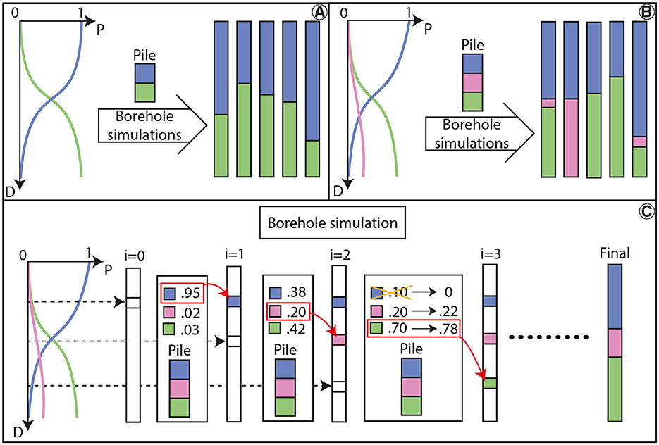
Figure 7. (A, B) Illustrated are examples of borehole simulation under two distinct settings. The curves depict the ML outputs, representing probabilities for each class as a function of depth. It is important to note that simulated boreholes are purely for illustrative purposes and do not reflect equiprobable simulations from the given curves. (C) Schematic representation of the workflow. The methodology iteratively identifies vacant intervals within the borehole and simulates the corresponding unit based on probabilities derived from ML. Notably, probabilities are adjusted in accordance with the existing stratigraphy, ensuring that units deemed impossible are assigned a probability of 0 (blue unit at iteration 2).

The adopted methodology follows the sequential algorithm proposed by Journel and Alabert [35], using ML for probability predictions. The process starts with an empty borehole, segmented into intervals identical to those in the facies log (refer to Figure 6). Subsequently, a random empty interval is chosen, and the trained ML algorithm is employed to obtain the predicted probabilities. On the basis of these probabilities, a unit is randomly drawn and assigned to the interval. This sequence is repeated iteratively, with additional intervals selected and filled until the entire borehole is populated. The particularity here is that probabilities are adapted according to the stratigraphic pile. This means that impossible to simulated units have a probability set to 0, while the others are rescaled. This step is shown in Figure 7C, iteration 2 where the only possible units are pink and green due to the previously simulated units (blue cannot be located below pink).

Note that, this simulation procedure might encounter a deadlock when all probabilities are reduced to 0. In such instances, the simulation is stopped and a new empty borehole is generated. To avoid being stuck, if the number of these errors exceeds a specified value (n_e, user defined), the borehole is deemed impractical to simulate.

Furthermore, ML predictions can exhibit significant noise, especially when dealing with a large number of units, resulting in numerous small probabilities assigned to a vast array of units. This noise can adversely affect the performance of the simulation algorithm, leading to artifacts characterized by numerous occurrences of units with small thickness. To address this issue, a filtering mechanism is implemented to remove probabilities below a certain threshold (τ, user-defined). This threshold should be set high enough to reduce noise, but a too large value reduces the variations in the simulated boreholes and can even lead to impossible simulations. After some trial and error, a value of 0.15 was identified as a suitable compromise for the boreholes within the study area.

3 Results

3.1 Machine learning

In Figure 8A, the mean metric values for different algorithms are compared. This shows the metrics of the ML algorithms on the test set based on the features (lithological and geographical) described in the previous subsection. Overall, all models exhibit reasonable performance, except Adaboost, which demonstrates notably low precision (20%) and a high Brier score (0.9). The remaining models show precision, recall, F-score, and Brier score values in the range of 0.5–0.6. In particular, MLP is marginally less accurate compared to others, exhibiting a higher Brier score that exceeds 0.6, while RF, SVC, and Gboost maintain scores below 0.55. This indicates that predictions made with MLP are overconfident, compared to the others. Figures 8B–D provide a detailed summary of the scores for each class for RF, SVC, and Gboost. It is blatant that certain classes, such as AM, OS, AS, or HB, are not accurately modeled. This discrepancy can be attributed to the low number of boreholes in the test set that contain these units, making the validation step less reliable. A similar situation is observed for IGT, which, despite having very good results, is represented by only one borehole in the test set. Consequently, assessing the reliability of the predictions for these units is not feasible. Fels unit, which represents the bedrock, has a perfect prediction for the only reason that this unit is characterized by a single and unique “lithology,” not integrated in the geological model, as it defines the bottom of the geological model. The other units exhibit decent results with precisions around 0.6 and 0.8. The Brier score is a bit more variable and can be near 0 (for GS) but can reach 0.75 (for UBS, Figure 8D).

Figure 8

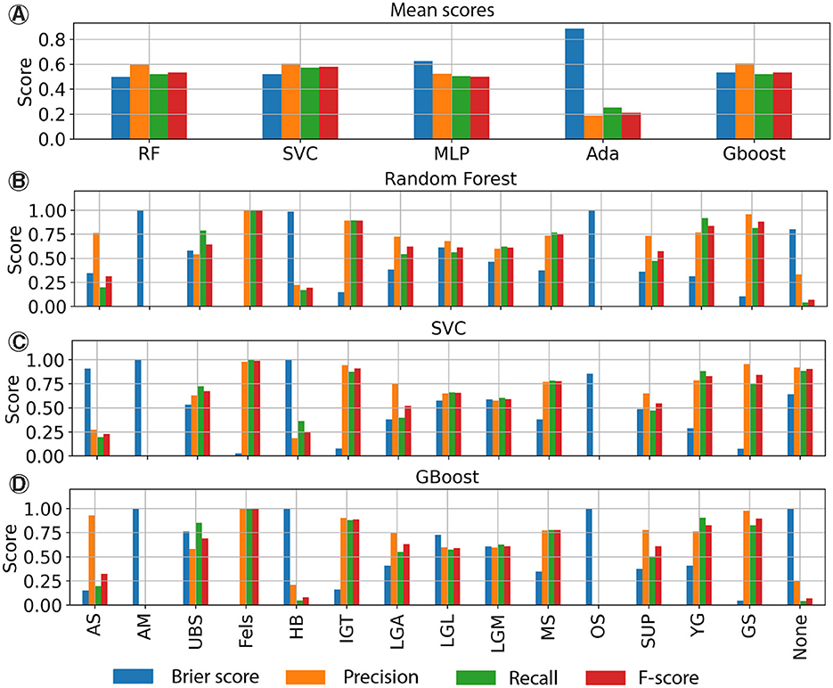
Figure 8. The following tables present the scores achieved by the ML algorithms on the test set. (A) Mean scores for all models. Each class was assigned the same weight. (B–D) Detailed scores for each class for the RF, SVC and Gboost algorithms.

We can add to this analysis the results obtained on testing ML algorithms on the training dataset, which is shown on Supplementary Figure S10. All methods give nearly perfect results on the training dataset, except again Adaboost and also SVC which exhibits an accuracy around 90%. These differences could indicate a potential over-fitting of the algorithms, despite the cross-validation, or that the data used for the training are not representative enough to capture all the non-linear relations between lithologies and stratigraphies.

To go further into depth and control that the borehole simulations produce reasonable results, Figure 9 shows the simulations for one borehole. 20 boreholes were simulated in each case and can be compared with the reference unit and facies logs. Predictions are close to the reference and three out of four methods are able to predict the reference borehole correctly. Only MLP predicts the SUP unit base too deep as compared to the reference. However, all methods were able to determine the transition between the aquifer and the aquiclude (YG and LGL) which is clear on the facies log. Note how the method is able to consider that there is a certain variety of lithologies in the YG aquifer unit where we find sands, clayey sands, gravels, and clayey gravels.

Figure 9

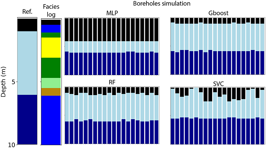
Figure 9. Borehole simulations for a 10 m depth borehole. Reference and facies log are shown to the left while simulations are shown to the right, each distinct bar corresponds to one simulation. The threshold used was set at 0.15, but if simulations were not feasible with this value, it was decreased until simulations were feasible. See Figure 4 for corresponding colors for unit and facies.

Figure 10 shows less satisfactory results from another borehole. The observations reveal that MLP and Gboost offer minimal variations, with outputs exhibiting near-deterministic behavior, in contrast to RF or SVC predictions. This is particularly visible on the predicted probabilities (Figure 10B). It is also quite clear that RF has more smooth probability transitions between different classes compared to the other methods. The reasons for these deterministic predictions are unclear and could be related to a possible over-fitting of these two methods (MLP and Gboost) and thus to the choice of hyperparameters, and/or directly related to the structure of these methods. For example, the sequential training of Gboost and MLP could lead to more rigid models and overconfident predictions, compared to parallel training of RF. The high number of layers (4) and neurons (nearly 1,000) in the MLP could also be the cause of over-fitting. With regard to the gradient boosting method, it corrects errors during training in order to improve accuracy on the training dataset [41]. However, this can cause over-fitting, leading to overconfident predictions. In the case of RF, the bagging (bootstrap sample of the training data) strategy for the learning process may assist in achieving more accurate probability predictions [47]. For SVC, it is known that it works well in high-dimensional problems [47, 48] and is less susceptible to over-fitting. This may account for the less certain, but more accurate probability predictions.

Figure 10

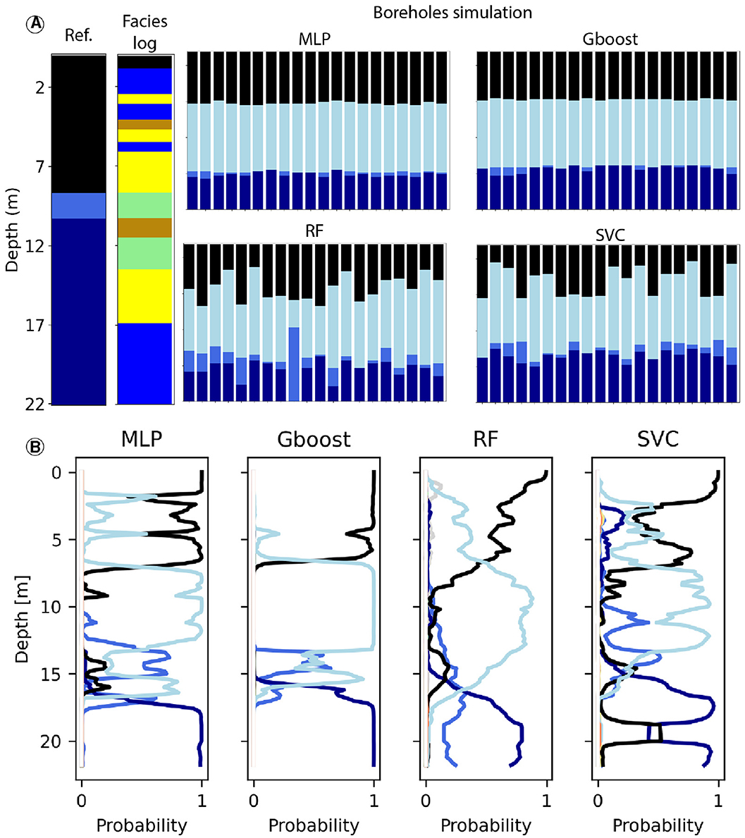
Figure 10. Simulations of another borehole. (A) Simulated boreholes by the different algorithms and comparison with the reference. (B) Predicted probabilities for all of the classes by the ML algorithms at the different depths of the borehole. The classes are represented by the colored squares on top of each subplots. See Figure 4 for corresponding colors for unit and facies.

None of the methods predict the reference borehole in any simulation (Figure 10A), as well as on the ML probability outputs (Figure 10B), but they provide reasonable results if we look at the lithological log. All methods predict the SUP unit from the surface to a depth of 5–7 m, similar to the reference. The lithologies, shown in the facies log, significantly influence the prediction of this unit, with clay, sand, and clayey sand, which is a common assemblage of lithologies for this unit. All models predict the main aquifer unit, young Aar gravels (YG), and a transition to late lacustrine deposits (LGL) around 17 m in depth. RF and SVC additionally forecast a thin layer of the LGA unit, albeit deeper than indicated by the reference borehole. Although the predictions do not align with the reference borehole, they make sense based on the lithological log that shows a clear transition between sand and clay lithologies around 17 m in depth.

For the sake of brevity, only simulations for two boreholes are shown, but several others can be found in the Supplementary material. For example, Supplementary Figures S12, S13 show that algorithms can give very different results that are completely different from each other. In the former case, algorithms predict two distinct units for the clay-rich layer at 7 m, where Gboost and RF suggest IGT while SVC proposes LGL (which is ultimately correct). Just above, Gboost and RF also suggest a blend of YG and MS with occasional LGA, while SVC predicts solely YG (which is also correct). In the case of Supplementary Figure 13, MLP and SVC anticipate a sequence of HB and LGL, while Gboost and RF foresee a sequence of YG and LGL (which aligns with the correct succession, as per the interpreted log).

In certain cases, the facies log provides limited information, as shown in Supplementary Figure S14, where the predominance of gravels complicates the differentiation between units. The models anticipate a succession of MS and UBS, both predominantly composed of gravels, with SVC even indicating some LGA at the top. Distinguishing between these units based on lithologies proves impractical, prompting models to depend on spatial features constrained by other boreholes. The UBS predictions in all models are likely attributed to one or more other boreholes containing a similar succession of units and facies.

Simulations in Supplementary Figures S15, S16 show that the algorithm is also able to predict the correct units (YG, LGA) even when the facies log provides limited information. Determining the transition between these two units is not straightforward as they both globally have the same proportions of facies (Figure 5). In such cases, the predictions are probably dictated by other boreholes that help to find the transition between two similar units such as YG and LGA.

It is also worth mentioning the effect of the extrapolation on the predicted results. Based on the map showing the spatial distribution of the test and training sets (Supplementary Figure S1), two boreholes are particularly outside the convex hull defined by the training boreholes. The results of these two boreholes are shown in Figures S18, S19. Excluding the red unit (Fels unit), which is simple to predict because it contains only one facies, the predictions are very different between the methods. On the two boreholes, MLP and Gboost have an accuracy of about 5%–10%, while RF has an accuracy of 57%, which is comparable to the average accuracy obtained on the other test data (see next section). However, SVC has a higher accuracy, reaching 72%. However, even if the fact that these data are outside the convex hull could partly explain some of the poor results obtained, the results obtained with SVC and RF show that the integration of non-spatial data (lithology) could help to mitigate the difficulty of extrapolate. However, the number of extrapolated wells is too small to draw any conclusions.

Despite the adoption of a flexible approach for simulating boreholes based on probabilities, there is no guarantee that a borehole can be successfully simulated if the predictions lack consistency. In particular, with RF models, only one borehole from the test set encountered this situation. In contrast, other models exhibited less favorable outcomes, with three failed simulations for SVC, six for Gboost, and a more substantial 15 for MLP. The root cause of these failures can be traced to overconfident predictions that restrict the necessary flexibility required for successful simulation.

Taking these findings into account, it appears that there are no large differences between SVC, Gboost, and RF in terms of standard metrics. However, RF shows a slightly lower Brier score than the others (0.49 vs. 0.53), while SVC excels in precision, recall, and F-score. Furthermore, visual inspection of the simulated boreholes seems to allow us to show that RF proposes better predictions with greater variability, compared to MLP and Gboost. RF also seems to propose more accurate simulations than SVC.

Based on these results, the preference is to continue with the RF algorithm over SVC, despite its lower recall and F-score. This choice aligns with the priority of favoring models that are not overly confident and retain a degree of uncertainty in their predictions. Since probability predictions are the focus rather than the most probable ones, it is deemed more appropriate to continue with models that demonstrate superior performance in terms of the Brier score.

3.2 Geological models

3.2.1 Comparison

In this section, we present the geological models obtained with and without the newly added ML boreholes, and compare the models using the test set boreholes. Moreover, the number of inconsistencies between facies data and simulated stratigraphic units are also compared. Two models are developed following the specifications detailed in Section 2.3: a basis model (ArchPy-BAS) that relies solely on boreholes from the training set, complemented by geological maps and cross-sections; and an ML-augmented model (ArchPy-ML) that is enhanced through the integration of ML-generated boreholes utilizing the tuned RF model described in the previous section.

It is important to note that the SUP unit may unintentionally fill the simulation grid near the surface, depending on the surface simulations. This is due to how ArchPy defines the unit domains, which depend on the top and bottom surfaces of each unit. For the SUP unit, the top surface is set at DEM to prevent unsimulated cells. However, this can result in a significant exaggeration of the SUP unit's thickness, depending on how the older unit surfaces (HG, YG, etc.) have been simulated. For consistency reasons, the final geological models excluded this unit as it was deemed irrelevant. In such cases the SUP unit simulated cells were assigned the unit of the nearest non-SUP unit cell.

The confusion matrix between the two models is shown in Figures 11A, B. Most of the units are relatively well simulated, except for AM, OS, and SUP. The main reason is the same as for ML algorithms validation, as the poor number of boreholes in the test set containing these units, particularly for AM and OS. Another reason is also the scarcity of the deposits which are only located in some part of the simulation domain. ArchPy-BAS model is slightly better than ArchPy-ML in terms of global predictions (66% vs. 64%), primarily due to BAS's better accuracy in reproducing the YG unit, while ArchPy-ML is better with LGL, LGA, and SUP units. However, ArchPy-BAS exhibits a worse Brier score (0.56 vs. 0.50), suggesting that the ML-enriched model offers less confident simulations and enhances uncertainty quantification.

Figure 11

Figure 11. Comparisons metrics between ArchPy-BAS and ArchPy-ML Aar geological models. (A, B) Show the normalized confusion matrix of the predicted classes against true (observed) classes in the test set for ArchPy-BAS and ArchPy-ML, respectively. (C, D) Depict the frequency of inconsistencies found in terms of lithological data within each unit domain.

ArchPy-ML models also decrease the number of “errors” (or inconsistencies) between facies data and simulated units as shown in the Figure 1. Inconsistencies can arise when a stratigraphic unit is missing from borehole logs. These errors can be quantified by comparing the number of cells where facies data are found within inconsistent, simulated stratigraphic units, as shown in SP (Figure 4). This is shown in Figures 11C, D. In total, the number of discrepancies decreases from 536 for the ArchPy-BAS model to 374 for the ArchPy-ML model. However, errors remain after the integration of ML boreholes. This is because the SP was constructed with the assumption that lithologies present in < 5% proportion were absent from a unit. This can lead to errors, as a lithology present in small proportions may cause these errors. This is clearly visible for the YG unit, which has low proportions of C and SC lithologies. These lithologies have not been considered as part of the unit, but their exclusion results in a high number of errors (Figures 11C, D), even with ML model. Therefore, these errors are included in the data and cannot be eliminated with the current approach. Possible causes of these occurrences include rare lithology inclusions in specific units or misinterpretation of either lithologies or units.

3.2.2 Final models

The previous results show that ML techniques can enhance geological modeling. To optimize the model's performance, the RF model was retrained, but using all the existing borehole data and utilized to simulate the boreholes. This subsection presents the models (ArchPy-BAS and ArchPy-ML) integrated with all available borehole data. A total of 50 realizations were made for each model, for each realization, one different ML borehole simulation is made.

Figure 12 provides information on the internal structures of the unit for the two models. In some cases, the boreholes shown on the cross sections do not exactly match the simulated values. This is because the boreholes shown are not exactly on the section, but at a maximum distance of 100 m from the section. In general, both models exhibit similar geological structures at shallower depths and greater depths. The shallow aquifer appears closer to the surface in the northern regions (~5–10 m) and gradually deepens toward the south (up to 50 m, locally reaching 100 m). Southern areas show low variability in geology, with a shallow aquifer overlaying LGM deposits, which in turn rest on older clay deposits (AS), indicating the absence of a deep aquifer in the south. On the contrary, the northern regions display more intricate stratigraphic sequences, suggesting the presence of aquifer formations (UBS, OS, MS) at intermediate depths, beneath the shallow aquifer (YG, LGA). Intermediate layers typically comprise LGL and IGT units. MS is not necessarily in contact with UBS, suggesting that the deep heterogeneity in this area is more complex than just a two-layered aquifer.

Figure 12

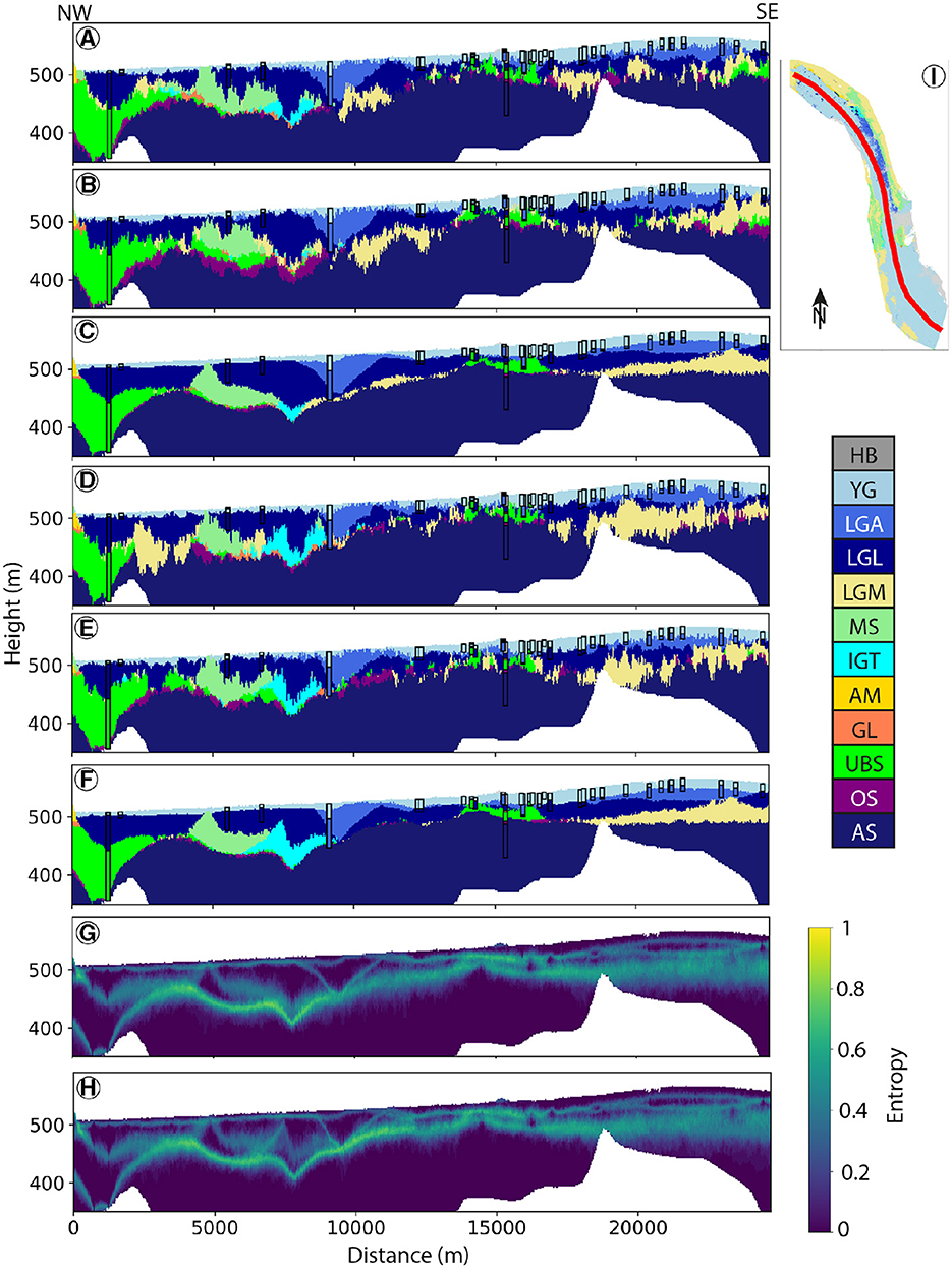
Figure 12. Longitudinal cross-section across two realizations of the ArchPy-BAS (A, B) and ArchPy-ML model (D, E). Cross-sections of highest indicator facies value for both models are also shown [(C) for ArchPy-BAS and (F) for ArchPy-ML]. Closest boreholes of the cross-section are displayed. The Shannon entropy is also shown for both models ((G) and (H) for ArchPy-BAS and ArchPy-ML, respectively). Location of the cross-section is illustrated in (I).

Although the two models share common features, discrepancies emerge particularly in the intermediate depths in the northern part of the area. ArchPy-ML simulations indicate a thicker presence of IGT compared to ArchPy-ML simulations in this region. This is more clear when observing the “most probable” models (Figures 12C, F for ArchPy-BAS and ArchPy-ML, respectively) that show the most probable unit in each cell according to the realizations. We see that the mean models are very close except around 7,500 m of distance, where the IGT layer is clearly thicker and present in ArchPy-BAS than in ArchPy-BAS model. Locally, we can note differences for the transition between YG-LGA-LGL units, but these are relatively rare.

Entropy values appear visually similar (Figures 12G, H); they do not indicate any significant reduction or increase in uncertainty. The only noticeable difference is that the ArchPy-ML model entropy is higher at intermediate depth between a distance of 10,000 and 13,000 m, suggesting a wider diversity in terms of units.

Transverse cross-sections (Supplementary Figures S20A–I and Figures 13A–I) offer more detailed insights. Similarly to previous observations (Figure 12, the ArchPy-ML model consistently depicts the IGT as thicker and more extensive in the northern part, compared to the ArchPy-BAS model (Figure 13D vs. Supplementary Figure S20D). Furthermore, small and very thin occurrences of certain units, particularly at the interface between two thick units (e.g., IGT vs. AS in Figure 13C), are more common in the ArchPy-BAS simulations compared to the ArchPy-ML model. Although only one simulation is presented per model here, these trends are observable across other realizations as well. Both models clearly show that the north appears to be more complex than the south, which is mainly represented by a succession of YG-LGA-LGL-LGM and AS, with some local deposits of OS and UBS. On the contrary, in the north, all units can be present, according to the models.

Figure 13

Figure 13. (A–I) Transversal cross-sections in one realization of the ArchPy-ML unit model. Corresponding locations are shown in (J). (K) 3D visualization of the realization. Corresponding color for units are given in Figure 4.

The two models exhibit minimal disparity in terms of lithologies and properties, with the primary distinction being the incorporation of unit logs. In particular, it is difficult to visually discern between the two facies models (see Supplementary Figure 21 and Figure 14). The 3D views (Supplementary Figure S21K vs. Figure 14K) suggest that clay facies (C) are more present at depth in ArchPy-ML than in ArchPy-BAS model. Although, despite employing a relatively straightforward facies modeling technique such as SIS, complex, intricate, and constrained facies and property simulations can be obtained.

Figure 14

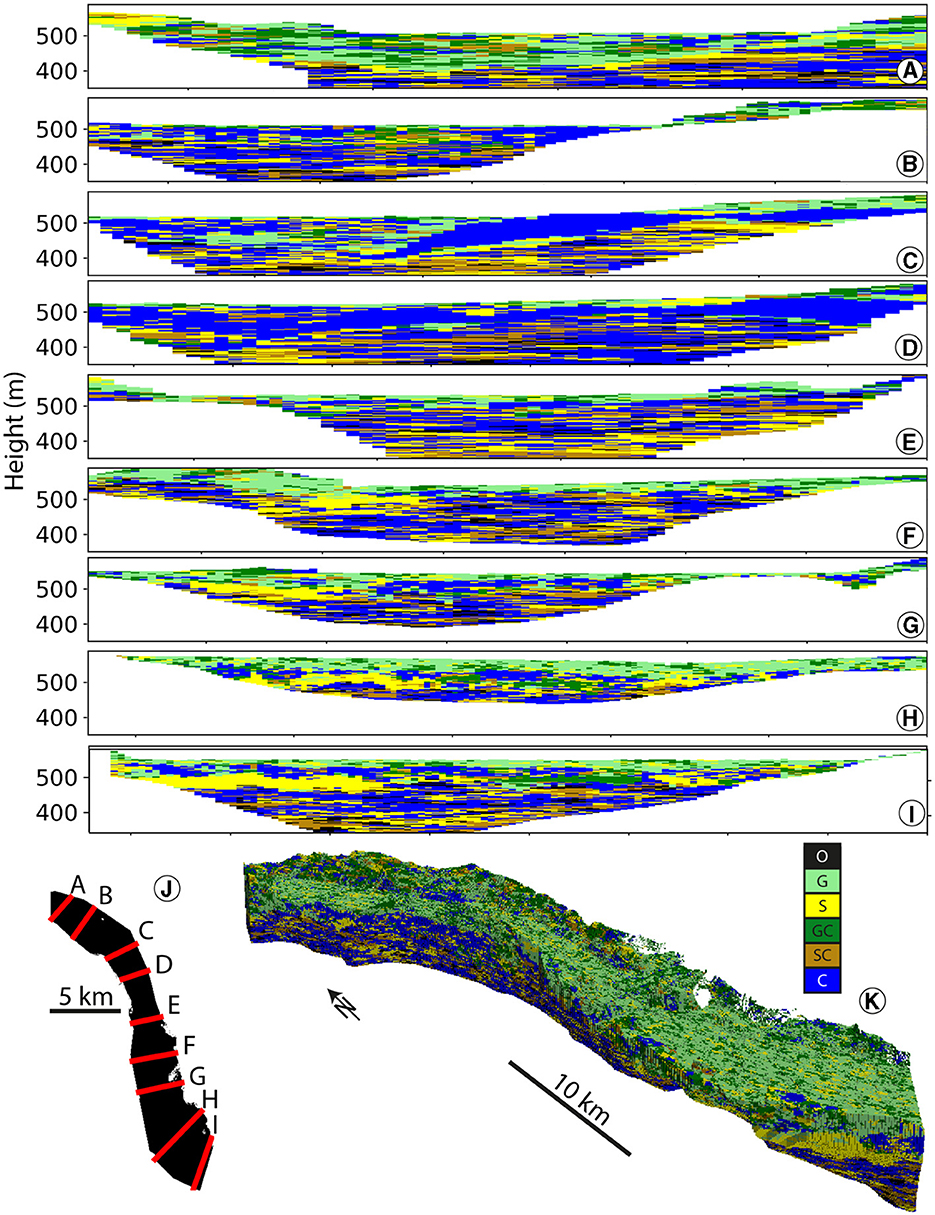
Figure 14. (A–I) Transversal cross-sections in one realization of the ArchPy-ML facies model. Corresponding locations are shown in (J). (K) 3D visualization of the realization. Corresponding color for facies are given in Figure 4.

Property models (see Supplementary Figure S22 and Figure 15) offer valuable information on the potential distribution of hydrogeological characteristics (aquifers and aquitards). The average hydraulic conductivity within the valley is ~$10^{-5}\left[\frac{m}{s}\right]$, but it greatly varies in space, both vertically and horizontally. The shallow aquifer is discernible near the surface with a conductivity of more than $10^{-3}\left[\frac{m}{s}\right]$, particularly in the southern region, where it exhibits a greater thickness (over 50 m). The presence of an impermeable layer between the superficial aquifer and the potential deep aquifer is clearly visible in the north and seems to have disappeared almost completely in the south. Although some deeper conductive lenses are observable (e.g., Figures 15F or C), conclusive evidence of a deep aquifer over the entire valley is lacking. In the south, the models suggest the presence of only one shallow and thick (50 m) aquifer. The geology in the north seems more complex, and possible vertical interactions between shallow and deep water reservoirs can be considered. It is essential to note that these models represent only averages and do not capture the complete heterogeneity of the subsurface. They provide information on areas that are likely to be more conductive to groundwater flow than others.

Figure 15

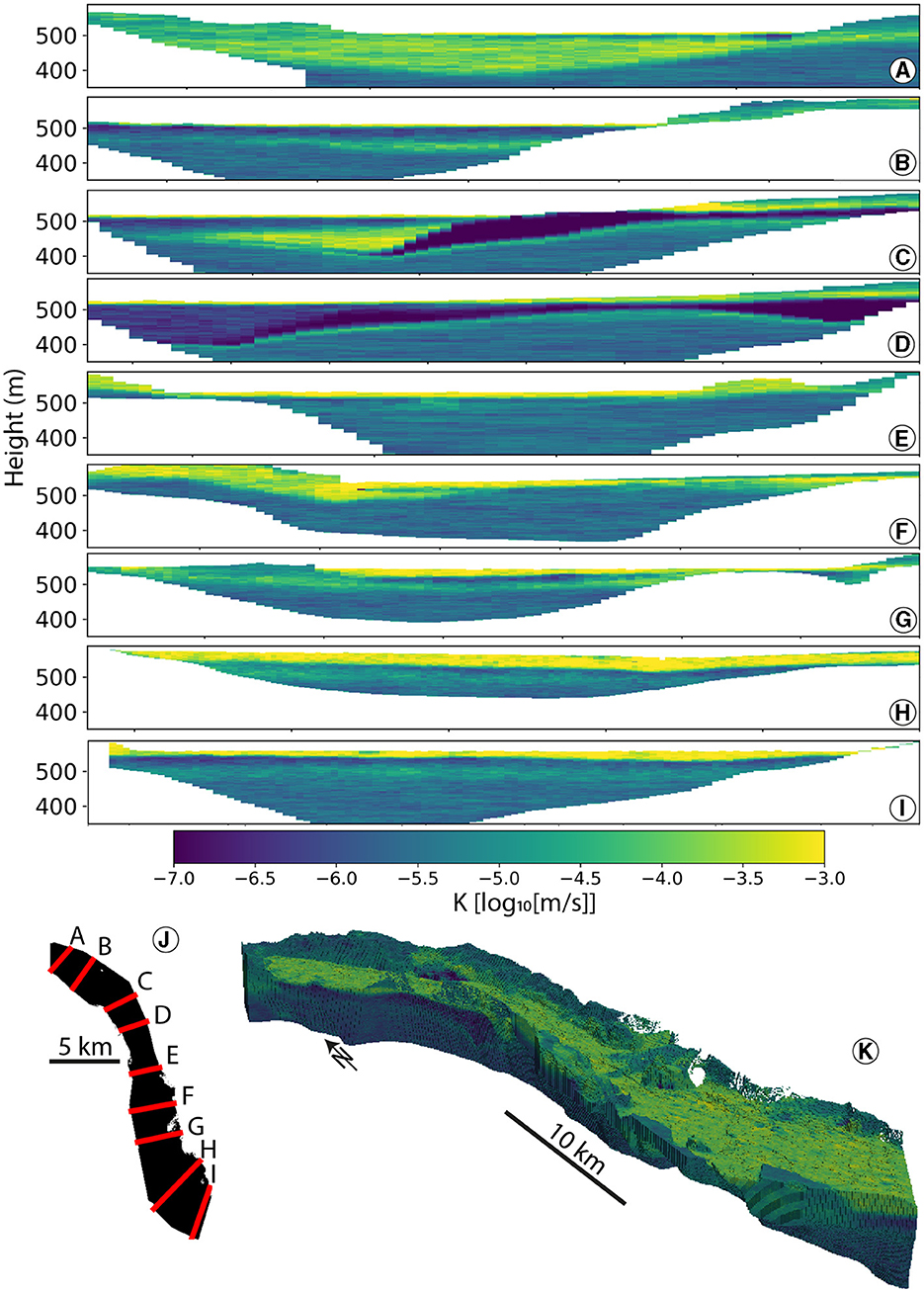
Figure 15. (A–I) Transversal cross-sections in mean of all property realizations of ArchPy-ML. Corresponding locations are shown in (J). (K): 3D visualization.

Between the two models, ArchPy-ML models exhibit a larger contrast, mainly due to the conductivity of the AS unit, which is lower than for ArchPy-BAS models. The reason is the proportion of the lithologies that are different between the two models. The integration of new unit ML generated logs has changed the proportions of the facies for each units. For rare units, such as AS, this was sufficient to provoke a reduction of the mean hydraulic conductivity by nearly one order of magnitude.

We can also compare models based on their “mean” unit and facies models (Supplementary Figures S23–S26). In these figures, the unit (or facies) that is shown in each cell is the one that has the most probability to appear according to the 50 realizations.

Unit models are very similar and only differ in some specific locations, particularly in the Northern part where the first cross-section with ArchPy-ML (Supplementary Figure S24A) shows a thicker GL unit than with BAS model (Supplementary Figure S23A). IGT unit is also thicker and widespread in ML model (Supplementary Figurer S24D) than in BAS model (Supplementary Figure S23D).

Mean facies models (Supplementary Figures S25, S26) are really useful as facies with highest proportions in each unit are presented which shows the difficulty to obtain a mean facies model and the risk to aggregate realizations using the “most probable” method. Nevertheless, aquifer, aquitards and aquicludes are clearly discernible which can help to identify zones with higher groundwater potential. Overall, the gravel facies is present close to the surface, with clay and silts at depth. There are no notable differences between the ML and BAS models.

4 Discussion

4.1 Geostatistical learning methodology

The methodology used to infer geological units was able to simulate reasonable stratigraphic units based on lithology information. Despite the complexity of the task, ML algorithms yield relatively decent results. In particular, the use of probabilistic ML outputs rather than deterministic predictions allowed us to introduce a level of uncertainty and preserve it through the modeling process.

Integration of a larger number of boreholes has improved the geological model, allowing better capture the spatial statistics of the surfaces that bound these units. Another interest of this methodology is that it can help detect or correct potentially erroneously interpreted wells, thereby improving the accuracy of geological models.

However, there are several challenges and areas of improvement remaining. In particular, the limited dataset size poses challenges in performing comprehensive cross-validation to assess the method's viability accurately. If the number of boreholes is consequent (791 in total and 266 labeled), they are not equally distributed over the modeling area and rarely exceed 50 m depth. This eventually reduces the quality of ML predictions for deep boreholes and also increases the uncertainty of geological models at intermediate and high depths. Grouping of lithologies and units also requires careful consideration to mitigate potential biases. It is possible that grouping all lithologies into six groups could remove patterns useful for predicting units. It is also important to mention that the definition of the facies and their grouping have to be done according to the modeling facies methods. Here we used SIS which is flexible and makes no supposition on deposit conditions, but if more advanced methods would have been employed such as Object-based or Rule-based methods, it is clear that a more detailed description of the data would be required.

In fact, the quality and homogenization of the data is another critical consideration. It is evident that improperly homogenized lithological logs can misguide ML algorithms. Specifically, the level of detail in descriptions varies widely because they originate from different companies, individuals, times, and purposes, complicating the homogenization process. In the case of the upper Aare Valley, these discrepancies exist and were not filtered or corrected prior to algorithm training, likely influencing the predictions. It is crucial to bear this in mind when interpreting the results.

Another clear limitation is that, overall, the simulation on the boreholes does not provide satisfactory results in all cases, which points to some limitations of the current approach. The roots of this problem can be partly attributed to the ML predictions that are on average quite low (around 50%–60%), with a high variability between the predicted classes. The reason for this are multiple. The lithologies were aggregated into six groups, which may have impacted the ML predictions, making them more difficult to estimate. Additionally, the approach involves a scanning window that provides lithological information 2 m above and below each elevation. Although this approach has the advantage of neglecting small facies occurrences, it also provides unnecessary information that makes it difficult to determine the transition between two units. Finally, the borehole simulation approach is not very robust and has limited global applicability. It requires the selection of a parameter (τ) and may generate artifacts in cases where multiple thin layers are simulated based on ML predictions. Furthermore, the method is predicated on the probabilistic outputs of ML algorithms, which are taken as truth. This may misguide some parts of the workflow and result in erroneous outcomes. A more thorough investigation into the integration of probabilistic ML outputs with existing or similar workflows could be beneficial.

However, it should also be noted that the prediction problem in this case is difficult where the relations between the 13 units with the lithologies and spatial coordinates are hard to make. It would be interesting to use this approach or an improved version on simpler synthetic cases to see in which situations the methodology works best, or on the contrary when it does not and how it can be improved. Overall, the problem addressed in this paper is of primal importance and the results obtained, despite unsatisfactory, are encouraging.

To address these issues, several improvements can be explored. Alternative feature strategies, such as integrating more lithologies above and below the target layers, adjusting layer thicknesses of each feature, and incorporating additional features (e.g., distance from the center of the valley, orientation data, geophysical data, predicted units at borehole location using ArchPy), could enhance model performance. Data augmentation, such as generating synthetic boreholes with ArchPy, could also be an option to adhere to stratigraphic rules and improve machine learning predictions. Investigating the SHapley Additive exPlanations (SHAP) [49] values could also help to investigate the impact of different features on the final results and may be an area for future research. In addition, instead of predicting units layer by layer, a direct prediction of surface elevation could provide a more efficient approach when coupled with the ArchPy borehole preprocessing algorithm [5]. To enhance the robustness of the borehole simulation step, a more robust and general approach should be taken. For instance, instead of using a random path, a deterministic path, going from the top to the bottom of the boreholes could be used. In a similar way, a Markov process could be employed, where transition probabilities are determined by the machine learning predictions. Alternatively, directly predicting the elevation of each unit's surfaces would eliminate the need for this step. Other ML methods could also be considered, such as neural networks, in particular Recurrent Neural Networks (RNN) [50], which are particularly useful for predicting a series of labels where outputs influence subsequent predictions, as is the case in a well log.

However, it is worth noting that the algorithm can make reasonable predictions in a good number of cases. For example, in the borehole depicted in Supplementary Figure S11, the transition between YG and LGL at a depth of 10 m is characterized by the appearance of a sand layer. However, since clays dominate the LGL, algorithms do not predict the transition at this depth. The same comment can be made in Supplementary Figure S12 where the transition between YG and LGL is predicted some meters below the reference (~10 m depth) because the lithological log shows a transition between sandy deposits to clayey deposits around 10 m depth. In such instances, the relevance of the data itself comes into question, prompting discussions of whether it is reasonable to pinpoint the transition at this precise depth or whether it would be more consistent to provide a range.

4.2 Geological models

The geological models show an intermediate uncertainty but that greatly varies in space. It is particularly high at intermediate depths (between 30 and 100 m), as shown by the entropy values (Figures 12G, H). This is logical because at shallow depth, geology is well known thanks to the numerous boreholes. On the opposite, in the deepest part, there is only one dominant unit, the AS. In between, the other units have a certain probability of appearing, depending on the boreholes and their covariance model. Although this uncertainty may seem high, it should be remembered that the geological complexity of the study area (13 units). Moreover, models provide stochastic simulations that consider this uncertainty and allow to propagate it through the subsequent modeling steps.

Indeed, it is important to emphasize that the prediction of geological units should not be viewed as an end in itself, but rather as a means to understanding the larger geological context. Imperfections in unit modeling are acceptable as long as they do not compromise the accuracy of the facies model (lithologies), which exert significant control over the distribution of properties in the subsurface. Therefore, it becomes imperative to dive deeper into this aspect to propose facies models that more accurately reflect the geological setting.

In this study, only the SIS method was considered for facies modeling. However, it should be noted that the inferring of variograms, particularly in the horizontal direction, posed significant challenges. Variogram parameters were determined primarily by trial and error, supplemented with expert knowledge of lithologies in the area. Unfortunately, such knowledge remains critically lacking for many units, leaving uncertainties that are difficult to address comprehensively.

As a result, the facies models can seem very uncertain, but it should be recalled that the resolution of the model is 25 m by 25 m, and it is very likely that the lithology heterogeneity displays a spatial range of heterogeneity below this value. Additionally, the SIS simulations were constrained in terms of facies proportions in each unit based on borehole data, but there is a high probability that these proportions are wrong due to a sampling bias. Drillers and local companies generally look for areas that have a high conductivity to better extract the water, as a consequence, the borehole generally stops when they reach large and thick clay and silty lithologies. Therefore, the proportions of sand and gravel in low permeable units are more likely to be overestimated.

The existence of a deep aquifer has been suggested and used as a working basis in several studies in the area [9, 24]. From the results obtained in this study (Figures 12, 13, 14, 15), it is difficult to assess the existence of a deep aquifer throughout the valley. However, we can clearly see that in the northern part of the area some conductive units (MS, UBS) seem to be present locally. YG and LGA, which are part of the shallow aquifer, are separated from these deeper units by LGL and IGT, suggesting that there are little to no exchanges between these two. These units seem to vanish as soon as the cross section in Supplementary Figure S22D. Some other deep conductive lenses (50–70 m) can be observed, such as the one in Supplementary Figure S22F but they are not widespread and are not observed in the other cross sections. All of this suggests that a second aquifer is likely to exist beneath the shallow one, but its extent is limited to the northern area. Its hydraulic conductivity is also expected to be lower as a result of the presence of more clayey deposits (SC, GC) compared to those of YG or LGA. To further characterize this lower aquifer, thresholds could be applied to hydraulic conductivity models to identify permeable areas. Probabilities of exceeding these thresholds could then be calculated. Or a numerical flow model could be used to study regional three-dimensional flows using these geological models.

In comparison of the ArchPy-BAS and ArchPy-ML models, both exhibit similar geological features. However, a notable difference emerges, particularly evident in property models (Supplementary Figure S22 and Figure 15): variable hydraulic conductivity for identical units. This discrepancy arises from the addition of ML-generated boreholes, which altered the lithological proportions within each unit. Consequently, certain units, such as AS, display a nearly one-order-of-magnitude difference in the simulated properties.

Hence, there is a great deal of room for improvement regarding geological models, mostly on the facies modeling part. Apart from other more complex methods (Multiple Point Statistics [51], Surface-based [52]) that can be employed, we can also imagine defining a more solid and complete geological conceptual model of the area, use of analogs for each unit, consider locally varying lithology proportions, etc. However, all of these steps would require an important amount of work that is beyond the scope of this research.

5 Conclusion

We presented a novel methodology for inferring stratigraphical unit logs based on lithological data using Machine Learning (ML). Several algorithms were tested, and it turned out that the Random Forest (RF) and Support Vector Machine (SVC) gave the best results in terms of accuracy and Brier score. The RF model was used to simulate consistent boreholes in areas where local stratigraphy data were missing. These simulated boreholes were then integrated into a geological model (ArchPy-BAS), resulting in an enhanced version (ArchPy-ML). The geological model operates on three hierarchical levels: stratigraphical units, lithologies (facies), and hydraulic conductivity properties. Although ArchPy-BAS exhibits marginally better accuracy than ArchPy-ML, the latter demonstrates superior performance in quantifying uncertainty, as indicated by its improved Brier score.

Visually, both models yield similar results, albeit with ArchPy-ML showing a greater presence of certain units, notably IGT. Analysis of these results enabled the determination of the lateral and vertical extent of potential deep aquifers. Our models suggest that their lateral spatial extent is limited and that there are uncertain connections between them. Furthermore, their hydraulic conductivity appears to be lower than that of the shallow aquifer, particularly in the south, where the aquifer is thicker. Exploiting these potential aquifers requires further investigation to obtain accurate estimates of their petrophysical properties.

This work also shows that there is room for further improvements. Identifying consistent stratigraphic data from lithological logs could be improved by involving probabilistic information or by using more advanced statistical learning techniques. It was also not possible during the timeframe of the research to integrate completely the geophysical data acquired by Neven et al. [33] in a large part of the valley. However, our approach still offers valuable information on the integration of ML with traditional geostatistical methods to improve the reliability of geological models. Ultimately, these advances contribute to improving the quality of groundwater models and understanding subsurface heterogeneity.

Data availability statement

The data analyzed in this study is subject to the following licenses/restrictions. The data used are the property of the Swiss Geological Survey (Swisstopo). Requests to access these datasets should be directed at: info@swisstopo.ch.

Author contributions

LS: Conceptualization, Investigation, Methodology, Software, Writing – original draft, Writing – review & editing. JS: Software, Supervision, Validation, Writing – review & editing. PR: Conceptualization, Funding acquisition, Methodology, Supervision, Validation, Writing – review & editing.

Funding

The author(s) declare that financial support was received for the research, authorship, and/or publication of this article. This research was funded by the Swiss National Science Foundation under the contract 200020_182600/1 (PheniX project).

Acknowledgments

The authors would like to thank the three reviewers who helped to improve the quality of this article.

Conflict of interest

The authors declare that the research was conducted in the absence of any commercial or financial relationships that could be construed as a potential conflict of interest.

Publisher's note

All claims expressed in this article are solely those of the authors and do not necessarily represent those of their affiliated organizations, or those of the publisher, the editors and the reviewers. Any product that may be evaluated in this article, or claim that may be made by its manufacturer, is not guaranteed or endorsed by the publisher.

Supplementary material

The Supplementary Material for this article can be found online at: https://www.frontiersin.org/articles/10.3389/fams.2024.1441596/full#supplementary-material

Footnotes

1. ^http://www.github.com/randlab/geone

References

1. Anderson MP, Woessner WW, Hunt RJ. Applied Groundwater Modeling: Simulation of Flow and Advective Transport. Cambridge, MA: Academic Press (2015).

Google Scholar

2. Pyrcz MJ, Deutsch CV. Geostatistical Reservoir Modeling. Oxford: Oxford University Press (2014).

Google Scholar

3. Koltermann CE, Gorelick SM. Heterogeneity in sedimentary deposits: a review of structure-imitating, process-imitating, and descriptive approaches. Water Resour Res. (1996) 32:2617–58. doi: 10.1029/96WR00025

Crossref Full Text | Google Scholar

4. Ringrose P, Bentley M. Reservoir Model Design, Vol. 467. Berlin: Springer (2016). doi: 10.1007/978-94-007-5497-3

Crossref Full Text | Google Scholar

5. Schorpp L, Straubhaar J, Renard P. Automated hierarchical 3D modeling of quaternary aquifers: the ArchPy approach. Front Earth Sci. (2022) 10:884075. doi: 10.3389/feart.2022.884075

Crossref Full Text | Google Scholar

6. Matheron G. Principles of geostatistics. Econ Geol. (1963) 58:1246–66. doi: 10.2113/gsecongeo.58.8.1246

Crossref Full Text | Google Scholar

7. Wellmann F, Caumon G. 3-D Structural geological models: concepts, methods, and uncertainties. In:Schmelzbach C, , editor. Advances in Geophysics, Vol. 59. Amsterdam: Elsevier (2018), p. 1–121. doi: 10.1016/bs.agph.2018.09.001

Crossref Full Text | Google Scholar

8. Neven A, Schorpp L, Renard P. Stochastic multi-fidelity joint hydrogeophysical inversion of consistent geological models. Front Water. (2022) 4:989440. doi: 10.3389/frwa.2022.989440

Crossref Full Text | Google Scholar

9. Neven A, Renard P. A novel methodology for the stochastic integration of geophysical and hydrogeological data in geologically consistent models. Water Resour Res. (2023) 59:e2023WR034992. doi: 10.1029/2023WR034992

Crossref Full Text | Google Scholar

10. Teles V, Bravard J, De Marsily G, Perrier E. Modelling of the construction of the Rhône alluvial plain since 15 000 years BP. Sedimentology. (2001) 48:1209–24. doi: 10.1046/j.1365-3091.2001.00419.x

Crossref Full Text | Google Scholar

11. Rigol JP, Jarvis CH, Stuart N. Artificial neural networks as a tool for spatial interpolation. Int J Geogr Inf Sci. (2001) 15:323–43. doi: 10.1080/13658810110038951

Crossref Full Text | Google Scholar

12. Kanevski M, Timonin V, Pozdnukhov A. Machine Learning for Spatial Environmental Data: Theory, Applications, and Software. Lausanne: EPFL Press (2009). doi: 10.1201/9781439808085

Crossref Full Text | Google Scholar

13. Zhang C, Sargent I, Pan X, Li H, Gardiner A, Hare J, et al. An object-based convolutional neural network (OCNN) for urban land use classification. Remote Sens Environ. (2018) 216:57–70. doi: 10.1016/j.rse.2018.06.034

Crossref Full Text | Google Scholar

14. Schratz P, Muenchow J, Iturritxa E, Richter J, Brenning A. Hyperparameter tuning and performance assessment of statistical and machine-learning algorithms using spatial data. Ecol Modell. (2019) 406:109–20. doi: 10.1016/j.ecolmodel.2019.06.002

PubMed Abstract | Crossref Full Text | Google Scholar

15. Fouedjio F, Klump J. Exploring prediction uncertainty of spatial data in geostatistical and machine learning approaches. Environ Earth Sci. (2019) 78:38. doi: 10.1007/s12665-018-8032-z

PubMed Abstract | Crossref Full Text | Google Scholar

16. Nikparvar B, Thill JC. Machine learning of spatial data. ISPRS Int J Geo-Inf . (2021) 10:600. doi: 10.3390/ijgi10090600

Crossref Full Text | Google Scholar

17. Szatmári G, Pásztor L. Comparison of various uncertainty modelling approaches based on geostatistics and machine learning algorithms. Geoderma. (2019) 337:1329–40. doi: 10.1016/j.geoderma.2018.09.008

Crossref Full Text | Google Scholar

18. Veronesi F, Schillaci C. Comparison between geostatistical and machine learning models as predictors of topsoil organic carbon with a focus on local uncertainty estimation. Ecol Indic. (2019) 101:1032–44. doi: 10.1016/j.ecolind.2019.02.026

Crossref Full Text | Google Scholar

19. Aliouane L, Ouadfeul S, Djarfour N, Boudella A. Lithofacies prediction from well logs data using different neural network models. In: Proceedings of the 2nd International Conference on Pattern Recognition Applications and Methods - Volume 1: PRG, (ICPRAM 2013). Setbal: SCITEPRESS (2013). p. 702–6. doi: 10.5220/0004380707020706

Crossref Full Text | Google Scholar

20. Hammond Z, Allen DM. Evaluating the feasibility of using artificial neural networks to predict lithofacies in complex glacial deposits. Hydrogeol J. (2024) 32:509–26. doi: 10.1007/s10040-023-02726-2

Crossref Full Text | Google Scholar

21. Sahoo S, Jha MK. Pattern recognition in lithology classification: modeling using neural networks, self-organizing maps and genetic algorithms. Hydrogeol J. (2017) 25:311. doi: 10.1007/s10040-016-1478-8

Crossref Full Text | Google Scholar

22. Zhou C, Ouyang J, Ming W, Zhang G, Du Z, Liu Z, et al. stratigraphic prediction method based on machine learning. Appl Sci. (2019) 9:3553. doi: 10.3390/app9173553

Crossref Full Text | Google Scholar

23. Li H, Wan B, Chu D, Wang R, Ma G, Fu J, et al. progressive geological modeling and uncertainty analysis using machine learning. ISPRS Int Geo-Inf . (2023) 12:97. doi: 10.3390/ijgi12030097

Crossref Full Text | Google Scholar

24. Kellerhals P, Haefeli C, Tröhler B. Grundlagen für Schutz und Bewirtschaftung der Grundwasser des Kantons Bern Hydrogeologie Aaretal, zwischen Thun und Bern. Bern: Wasser- u. Energiewirtschaftsamt des Kantons Bern (1981).

Google Scholar

25. Haeuselmann P, Granger DE, Jeannin PY. Lauritzen SE. Abrupt glacial valley incision at 08 Ma dated from cave deposits in Switzerland. Geology. (2007) 35:143–6. doi: 10.1130/G23094A

Crossref Full Text | Google Scholar

26. Schlüchter C. The most complete quaternary record of the Swiss Alpine Foreland. Palaeogeogr Palaeoclimatol Palaeoecol. (1989) 72:141–6. doi: 10.1016/0031-0182(89)90138-7

Crossref Full Text | Google Scholar

27. Preusser F, Schlüchter C. Dates from an important early late pleistocene ice advance in the Aare Valley, Switzerland. Eclogae Geol Helv. (2004) 97:245–53. doi: 10.1007/s00015-004-1119-4

Crossref Full Text | Google Scholar

28. Preusser F, Graf HR, Keller O, Krayss E, Schlüchter C. Quaternary glaciation history of Northern Switzerland E&G. Quat Sci J. (2011) 60:282–305. doi: 10.3285/eg.60.2-3.06

Crossref Full Text | Google Scholar

29. Graf HR, Burkhalter R. Quaternary deposits: concept for a stratigraphic classification and nomenclature—an example from Northern Switzerland. Swiss J Geosci. (2016) 109:137–47. doi: 10.1007/s00015-016-0222-7

Crossref Full Text | Google Scholar

30. Volken S, Preisig G, Gaehwiler M. GeoQuat: Developing a system for the sustainable management, 3D modelling and application of quaternary deposit data. Swiss Bull Appl Geol. (2016) 21:3–16. doi: 10.5169/seals-658182

Crossref Full Text | Google Scholar

31. Casagrande A. Classification and identification of soils. Trans Am Soc Civil Eng. (1948) 113:901–30. doi: 10.1061/TACEAT.0006109

Crossref Full Text | Google Scholar

32. Neven A, Christiansen AV, Renard P. Automatic stochastic 3D clay fraction model from tTEM survey and borehole data. Sci Rep. (2022) 12:17112. doi: 10.1038/s41598-022-21555-z

PubMed Abstract | Crossref Full Text | Google Scholar

33. Neven A, Maurya PK, Christiansen AV, Renard P. tTEM20AAR: a benchmark geophysical data set for unconsolidated fluvioglacial sediments. Earth Syst Sci Data. (2021) 13:2743–52. doi: 10.5194/essd-13-2743-2021

Crossref Full Text | Google Scholar

34. Chiles JP, Delfiner P. Geostatistics: Modeling Spatial Uncertainty, Vol 713. Hoboken, NJ: John Wiley & Sons. (2012). doi: 10.1002/9781118136188

Crossref Full Text | Google Scholar

35. Journel AG, Alabert FG. New method for reservoir mapping. J Pet Technol. (1990) 42:212–8. doi: 10.2118/18324-PA

PubMed Abstract | Crossref Full Text | Google Scholar

36. Deutsch CV, Journel AG. Geostatistical Software Library and User's Guide, Vol 119, 1st Edn. Oxford: Oxford University Press. (1992).

Google Scholar

37. Das BM, Sobhan K. Principles of Geotechnical Engineering. Boston, MA: PWS-Kent Publishing Company (1990).

Google Scholar

38. Fogg GE, Noyes CD, Carle SF. Geologically based model of heterogeneous hydraulic conductivity in an alluvial setting. Hydrogeol J. (1998) 6:131–43. doi: 10.1007/s100400050139

Crossref Full Text | Google Scholar

39. Breiman L. Random forests. Mach Learn. (2001) 45:5–32. doi: 10.1023/A:1010933404324

Crossref Full Text | Google Scholar

40. Freund Y, Schapire RE. A desicion-theoretic generalization of on-line learning and an application to boosting. In:Vitnyi P, , editor. European Conference on Computational Learning Theory. Berlin: Springer (1995), p. 23–37. doi: 10.1007/3-540-59119-2_166

Crossref Full Text | Google Scholar

41. Friedman JH. Greedy function approximation: a gradient boosting machine. Ann Stat. (2001) 29:1189–32. doi: 10.1214/aos/1013203451

PubMed Abstract | Crossref Full Text | Google Scholar

42. Haykin S. Neural Networks: A Comprehensive Foundation. Upper Saddle River, NJ: Prentice Hall (1998).

Google Scholar

43. Cortes C, Vapnik V. Support-vector networks. Mach Learn. (1995) 20:273–97. doi: 10.1007/BF00994018

Crossref Full Text | Google Scholar

44. Pedregosa F, Varoquaux G, Gramfort A, Michel V, Thirion B, Grisel O, et al. Scikit-learn: machine learning in Python. J Mach Learn Res. (2011) 12:2825–30. doi: 10.48550/arXiv.1201.0490

Crossref Full Text | Google Scholar

45. Brier GW. Verification of forecasts expressed in terms of probability. Monthly weather review. (1950) 78:1–3.2. doi: 10.1175/1520-0493(1950)078&lt;0001:VOFEIT&gt;2.0.CO;2

PubMed Abstract | Crossref Full Text | Google Scholar

46. Juda P, Renard P, Straubhaar J. A framework for the cross-validation of categorical geostatistical simulations. Earth Space Sci. (2020) 7:e2020EA001152. doi: 10.1029/2020EA001152

Crossref Full Text | Google Scholar

47. Hastie T, Tibshirani R, Friedman JH, Friedman JH. The Elements of Statistical Learning: Data Mining, Inference, and Prediction, Vol 2. Berlin: Springer (2009). doi: 10.1007/978-0-387-84858-7

Crossref Full Text | Google Scholar

48. Sarker IH. Machine learning: Algorithms, real-world applications and research directions. SN Comput Sci. (2021) 2:160. doi: 10.1007/s42979-021-00592-x

PubMed Abstract | Crossref Full Text | Google Scholar

49. Lundberg SM, Lee SI. A unified approach to interpreting model predictions. In:Guyon I, Luxburg UV, Bengio S, Wallach H, Fergus R, Vishwanathan S, et al., , editors. Advances in Neural Information Processing Systems 30. Red Hook, NY: Curran Associates, Inc. (2017), p. 4765–74. Available online at: http://papers.nips.cc/paper/7062-a-unified-approach-to-interpreting-model-predictions.pdf

Google Scholar

50. Rumelhart DE, Hinton GE, Williams RJ. Learning internal representations by error propagation, parallel distributed processing, explorations in the microstructure of cognition, ed. DE Rumelhart, J McClelland, Vol. 1. Biometrika. (1986) 71:599–607.

Google Scholar

51. Mariethoz G, Renard P, Straubhaar J. The direct sampling method to perform multiple-point geostatistical simulations. Water Resour Res. (2010) 46. doi: 10.1029/2008WR007621

Crossref Full Text | Google Scholar

52. Schorpp L, Straubhaar J, Renard P. A novel surface-based approach to represent aquifer heterogeneity in sedimentary formations. ESS Open Archive. doi: 10.22541/essoar.170612218.80961459/v1

PubMed Abstract | Crossref Full Text | Google Scholar