New alpha power transformed beta distribution with its properties and applications

The main purpose of this paper is to introduce a new alpha power transformed beta probability distribution that reveals interesting properties. The studuy provide a comprehensive explanation of the statistical characteristics of this innovative model. Various properties of the new distribution were derived, using the baseline beta distribution, statistical techniques, and probabilistic axioms. These include the probability density, cumulative distribution, survival function, hazard function, moments about the origin, moment generating function, and order statistics. For parameter estimation, the maximum likelihood estimation method using Newton Raphson numerical technique is employed. To evaluate the performance of our estimation method, the mean squared errors of the estimated parameters for different simulated sample sizes are used. In addition simulation studies of the new distribution are conducted to demonstrate the behavior of the probability model. To demonstrate the practical utility and flexibility of the alpha power transformed beta distribution, it is fitted to two real-life datasets and compared to commonly known probability distributions such as the Weibull, exponential Weibull, Beta, and Kumaraswamy beta distributions. It offers a superior fit to the data considered. The distribution reviales of the microbes reveald a wide range of shapes of probability density functions and flexible hazard rates. The distribution is a new contribution to the field of statistical and probability theory. The findings of the study can be used as a basis for future research in the area of statistical science and health.

1 Introduction

The beta distribution is a versatile tool in statistical modeling, known for its flexibility in reflecting various phenomena. It is defined by shape parameters a and b, ideal for modeling values between 0 and 1 like probabilities and proportions [1]. This distribution is valuable in reliability analysis of engineering systems, lifetime analysis and quality control in manufacturing [31]. In Bayesian statistics, the beta distribution is the conjugate prior for event probabilities in binomial processes [2, 3]. Scholars have parametrized it in different ways for effective modeling. The beta distribution is versatile, modeling various uncertainties with characteristics like unimodal or uniantimodal shapes, depending on shape parameters [2, 4].

The two-parameter beta distribution is not recommended for accurate data fitting [31], prompting the need for more adaptable forms to comprehensively represent data [5]. Expanding classic distributions, especially for lifetime data analysis, is essential [5]. Recent advancements in distribution theory, introducing additional parameters, have enhanced flexibility in modeling positive fraction numbers between zero and one [5]. Adding an extra parameter improves data fitting accuracy and reliability in statistical models [35], with approaches including modifying existing generators [5, 30] or developing new techniques for more extensive modifications [5, 30].

Researchers have introduced various exponentiated distributions, such as those by Gupta et al. [32] and Marshall and Olkin [30]. Different techniques, like the T-X class by Aljarrah et al. [6] and models using the logit function by Al-Aqtash et al. [7], have been proposed. Cordeiro et al. [8] introduced a new family using the quantile function of the generalized lambda distribution. The Muth-G distribution was proposed by Almarashi and Elgarhy [9], and Khalil et al. [35]) introduced the modified Frechet distribution for new continuous probability distributions.

Recently, Mahdavi and Kundu [10] developed a method for proposing a new probability distribution which is referred to as the alpha power transformation (APT) of the base distribution. Given the base cumulative distribution function G(x) and probability density function g(x) of the random variable X, the new commulative density function (CDF) and the corresponding probability density function (PDF) of the transformed random variable Y can be expressed as follows:

$\begin{array}{ll}G(y;\alpha )=\{\begin{array}{c}\frac{{\alpha }^{F(y)}-1}{\alpha -1}if\alpha >0,\alpha \ne 1\\ F(y)elseif\alpha =1\end{array}& (1)\end{array}$

$\begin{array}{ll}g(y;\alpha )=\{\begin{array}{c}\frac{ln(\alpha )}{\alpha -1}{\alpha }^{F(y)}f(y)if\alpha >0,\alpha \ne 1\\ f(y)elseif\alpha =1\end{array}& (2)\end{array}$

Researchers have introduced modifications like the three-parameter model by Chotikapanich et al. [11] and the four-parameter generalized beta model by Ng et al. [2] to enhance its applicability in data fitting. McDonald and Richards [12] and Libby and Novick [13] have also proposed alternative parameterizations of the beta distribution. Exton [33] introduced a generalized beta distribution with (2n + 2) parameters.

This study introduces the APT_beta distribution, a new generalization of the beta distribution using the alpha power transformation method. By addressing limitations of existing distributions, it enhances flexibility in data fitting with an additional parameter and relies on standard distribution's cumulative distribution for effectiveness [10, 36].

2 The alpha power transformation of the beta distribution

The base beta distribution of random variable X we want to consider has two parameters a, b > 0 and assumes values between 0 and 1 and has a probability density function (PDF) and commulative density function (CDF) respectively given by:

$\begin{array}{ll}f(x;a,b)=\frac{1}{B(a,b)}{x}^{a-1}{(1-x)}^{b-1}& (3)\end{array}$

$\begin{array}{ll}F(x;a,b)=\frac{1}{B(a,b)}{\displaystyle {\int }_0^x}{t}^{a-1}{(1-t)}^{b-1}dt& (\mathrm{4a})\end{array}$

Note that the beta distribution function F(x; a, b) has alternative representations that are suitable for computations as well. The commulative density function (CDF) is related to the beta function B(.), gamma function Γ(.), incomplete beta function B_y(.), and incomplete beta function ratio I_y(.) as follows:

$\begin{array}{r}B(a,b)={\displaystyle {\int }_0^1}{(1-t)}^{b-1}{t}^{a-1}dt=\frac{\Gamma (a)\Gamma (b)}{\Gamma (a+b)}\\ B_x(a,b)={\displaystyle {\int }_0^x}{t}^{a-1}{(1-t)}^{b-1}dt,I_x(a,b)=\frac{B_x(a,b)}{B(a,b)}\\ F(x;a,b)=\frac{1}{B(a,b)}{\displaystyle {\int }_0^x}{t}^{a-1}{(1-t)}^{b-1}dt\\ =\frac{B_x(a,b)}{B(a,b)}=I_x(a,b)& (\mathrm{4b})\end{array}$

The beta CDF can also be represented by using the Gauss hypergeometric function ₂F₁(.) as:

$\begin{array}{ll}F\left(x;a,b\right)=y^a{}_2{{\displaystyle F}}_1\left(a,1-b,1+a,x\right)/aB(a,b)& (\mathrm{4c})\end{array}$

where the Gauss hypergeometric function defined in Rainville [37] as follows:

$\begin{array}{l}{}_2{{\displaystyle F}}_1\left(a,1-b,1+a,x\right)=\frac{{\left(a\right)}_n{\left(1-b\right)}_n{x}^n}{{\left(1+a\right)}_{n}n!},\left|x\right|<1\end{array}$

A new random variable Y is generated by the alpha power transformation of the base beta distribution in Equations 3, 4 and it has a cumulative distribution function F_APT(y; a, b, α) and density function f_APT(y; a, b, α) given in Equations 5, 6. We call this the alpha power transformed beta (APT_Beta) distribution.

Definition: The cumulative distribution and density functions of the alpha power transformed beta (APT_Beta) distribution of the trandformed random variable Y based on Equations 1, 2 by 10 are given by:

$\begin{array}{ll}{F}_{APT}(y;a,b,\alpha )=\frac{{\alpha }^{\frac{1}{B(a,b)}{\displaystyle {\int }_0^y}{t}^{a-1}{(1-t)}^{b-1}dt}-1}{\alpha -1}& (5)\end{array}$

$\begin{array}{ll}{f}_{APT}(y;a,b,\alpha )=\frac{{ln(\alpha )\alpha }^{I_y(a,b)}{y^{(a-1)}(1-y)}^{(b-1)}}{(\alpha -1)B(a,b)}& (6)\end{array}$

where 0 < y < 1, a > 0, b > 0, and, α > 0, α ≠ 1.

$I_y(a,b)=\frac{1}{B(a,b)}{\int }_0^y{t}^{a-1}{(1-t)}^{b-1}dt$ is an incomplete beta function ratio, and $B(a,b)={\int }_0^1{t^{a-1}(1-t)}^{b-1}dt$ is the beta function. When α = 1 the APT_Beta distribution assumes the base CDF and PDF in Equations 3, 4.

Note that an alternative representation of the new CDF in Equation 5 and PDF in Equation 6 can be represented using the Gauss hypergeometric function. The new CDF can be represented using the Gauss hypergeometric function as follows:

$\begin{array}{ll}{F}_{APT}(y;a,b,\alpha )=\frac{{(\alpha )}^{\frac{y^{a}2F1(a,1-b,1+\alpha ,y)}{aB(a,b)}}}{(\alpha -1)}& (7)\end{array}$

The PDF of the APT_Beta distribution can be expressed interms of the Gaussian hypergeometric function from Wolfram computation as follows:

$\begin{array}{ll}{f}_{APT}(y;a,b,\alpha )=\frac{{ln(\alpha )(\alpha )}^{\frac{y^{a}2F1(a,1-b,1+\alpha ,y)}{aB(a,b)}}{(1-y)}^{b-1}{y}^{a-1}}{(\alpha -1)B(a,b)}& (8)\end{array}$

3 Plots of the APT_Beta probability distribution

The probability density function (PDF), cumulative density function (CDF), survival and hazard rate function plots for the APT_Beta distribution are given in list of figures in Appendix specifically in Figures 1–3, Supplementary Figure 3 respectively, for several different parameter values.

Figure 1

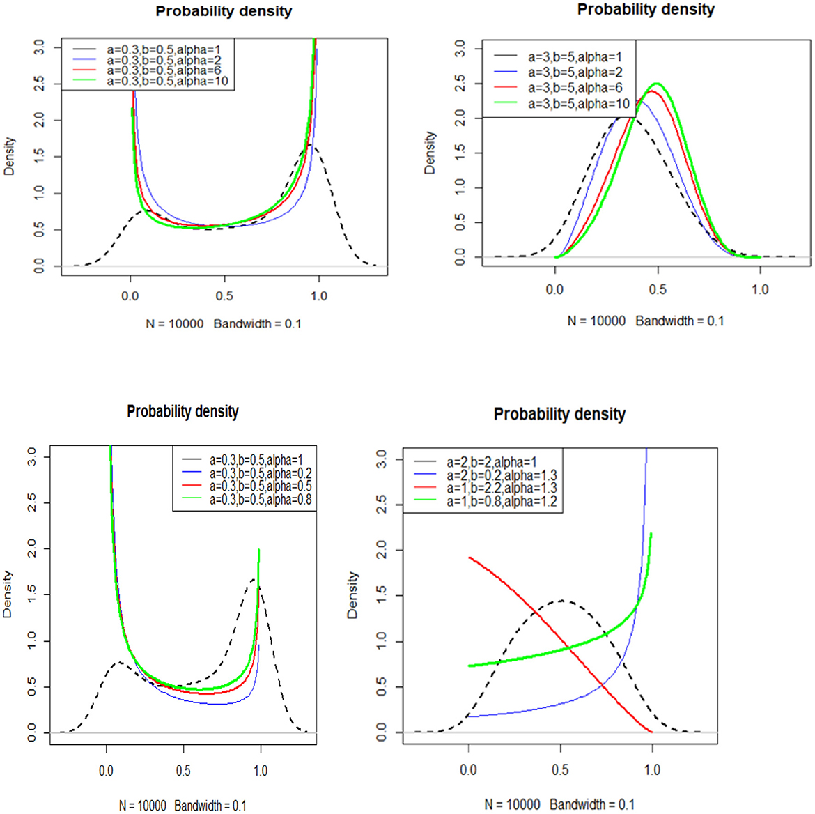
Figure 1. Plots of the APT_Beta density function for various values of parameters a, b, and α.

The density function has increasing, decreasing, left-skewed, right-skewed, J- shaped, U- shaped and approximately symmetric shapes, as shown in Figure 1. Our model's advantage is that it provides a wide range of shapes without requiring any additional parameters in its formulation. The new distribution provides more flexible shapes (see color plots) than does the base beta distribution (see black dotted plot) in the above density function plots at several values of a, b, and α. Especially the last three plots of Figure 1 shows that complete flexibility of the new distribution.

3.1 Plots of cumulative function of APT_Beta

The cumulative function plot in Figure 2 shows a twisted increasing graph that represents the cumulative distribution.

Figure 2

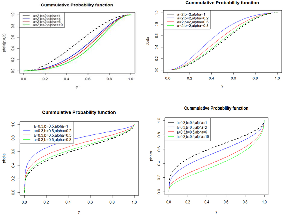
Figure 2. Cumulative distribution of APTB for various a, b, and alpha values.

4 Special cases of APT-Beta distribution

Case 1: If we consider the random variable Y, which follows the APT_Beta distribution with parameters a = 1 and b = 1, and a new parameter α ≠ 1, then the resulting distribution in Equation 6 exhibits the properties of an exponential function with a constant α as follows

$\begin{array}{l}{f}_{APT}(y;a=1,b=1,\alpha )=\frac{ln(\alpha )}{\alpha -1}{\alpha }^y;\\ a=1,b=1,\alpha \ne 1,\alpha >0,\left|y\right|<1& (9)\end{array}$

Proof

consider α be any real number such that α > 0 and α ≠ 1, then for any real number Y, a function of the form f(y) = α^y is called an exponential function [14].

$\begin{array}{r}{f}_{APT}(y;a=1,b=1,\alpha )=\frac{ln(\alpha )}{\alpha -1}\left({\alpha }^{I_Y(a=1,b=1)}\right)\\ \frac{1}{B(a=1,b=1)}{y}^{a-1}{(1-y)}^{b-1};\alpha \ne 1,\left|y\right|<1\\ f_{APT}(y;a=1,b=1,\alpha )=\frac{ln(\alpha )}{\alpha -1}{\alpha }^y\end{array}$

Case 2: Assume that the random variable Y has an APT_Beta distribution with b = 1, a ∈ (2, 3,…..) and α > 0, α ≠ 1 positive integer number, then the APT_Beta distribution simplifies and is defined as

$\begin{array}{r}{f}_{APT}(y;a,b=1,\alpha )=\frac{a^{*}ln(\alpha )}{\alpha -1}({\alpha }^{y^a})y^{a-1};\\ (a,\alpha >0),b=1,\alpha \ne 1,\left|y\right|<1& (10)\end{array}$

when α = 1 it is simplified to a polynomial function with |y| < 1 as follows

$\begin{array}{ll}{f}_{APT}(y;a,b=1,\alpha =1)=a{y}^a& (11)\end{array}$

Proof

When α = 1, then the distribution becomes basic beta and b = 1 provides the polynomial function expressed as f(y) = ay^a [15]

$\begin{array}{l}{f}_{APT}(y;a,b=1,\alpha =1)=\frac{1}{B(a,b=1)}{y}^{a-1}=a{y}^a\end{array}$

When the alpha value is different from one, the probability density of the APT_Beta distribution is defined as follows

$\begin{array}{r}{f}_{APT}\left(y;a,b,\alpha \right)=\frac{ln\left(\alpha \right)}{\alpha -1}\left({\alpha }^{I_Y\left(a,b=1\right)}\right)\\ \frac{1}{B\left(a,b=1\right)}{y}^{a-1}{\left(1-y\right)}^{1-1};ifa\ne 1,b=1,\alpha \ne 1,\left|y\right|<1\\ f_{APT}\left(y;a,b,\alpha \right)=\frac{ln\left(\alpha \right)}{\alpha -1}\left({\alpha }^{\frac{1}{B\left(a,b=1\right)}{\displaystyle {\int }_0^y}{x}^{a-1}dx}\right)\\ \frac{1}{B\left(a,b=1\right)}{y}^{a-1};ifa\ne 1,b=1,\alpha \ne 1,\left|y\right|<1\end{array}$

where B(a, b = 1)$={\int }_0^1{y}^{a-1}dy=1/a$ and ${\int }_0^y{x}^{a-1}dx=y^a/a$

Therefore $f_{APT}(y;a,b=1,\alpha )=\frac{a^{*}ln(\alpha )}{\alpha -1}({\alpha }^y)y^{a-1}$

the proof is complete. The corresponding cumulative function becomes

$\begin{array}{r}{F}_{APT}(y;a,b=1,\alpha \ne 1)\\ ={\displaystyle {\int }_0^{\infty }}\frac{a^{*}ln(\alpha )}{\alpha -1}({\alpha }^{y^a})y^{a-1}dy=\frac{{\alpha }^{y^a}-1}{\alpha -1}\\ F_{APT}(y;a,b=1,\alpha \ne 1)=\frac{{\alpha }^{y^a}-1}{\alpha -1};\\ a,\alpha >0,a\ne 1,\alpha \ne 1,\left|y\right|<1\\ F_{APT}(y;a,b=1,\alpha =1)=\frac{a{y}^{a+1}}{a+1}\end{array}$

Case 3: For a random variable Y with a ≠ 1, b ≠ 1 and α = 1, the distribution becomes a basic beta distribution as shown in Equation 4.

Case 4: Consider a random variable Y having the APT_Beta distribution with exponent a as the whole number a = (2, 3, 4, ….) and b = 1, then the Weibull G-family expression of the APT_Beta distribution is [16]

$\begin{array}{c}{F}_{APTWG(y)}\\ =\{\begin{array}{c}({\alpha }^{y^n}-1)/(\alpha -{\alpha }^{y^n});if\alpha \ne 1,a,b,\alpha >0,0<y<1\\ \frac{F\left(y;a,b,\alpha \right)}{1-F\left(y;a,b,\alpha \right)}=\frac{y^a}{1-y^a}=\frac{y^n}{1-y^n};if\alpha =1,b=1,\alpha >0,\left|y\right|<1\end{array}& (12)\end{array}$

Proof

For any given continuous baseline distribution with commulative distribution F(y), one can drive the Weibull-G family distribution by F(y)/(1-F(y)) (Equation 16). Therefore the APT_Beta Weibull-G family commulative becomes

$\begin{array}{r}odsratio=\frac{F(y;a,b,\alpha )}{1-F(y;a,b,\alpha )}=\frac{\frac{1}{B(a,b)}{\displaystyle {\int }_0^y}{x}^{a-1}{(1-x)}^{b-1}dx}{1-\frac{1}{B(a,b)}{\displaystyle {\int }_0^y}{x}^{a-1}{(1-x)}^{b-1}dx}\\ \frac{F(y;a,b,\alpha )}{1-F(y;a,b,\alpha )}=\frac{y^a}{1-y^a}=\frac{y^n}{1-y^n}\end{array}$

and

$\begin{array}{l}\frac{F_{APT}\left(y;a,b,\alpha \right)}{1-F_{APT}\left(y;a,b,\alpha \right)}=\frac{\frac{{\left(\alpha \right)}^{\frac{1}{B\left(a,b\right)}{\displaystyle {\int }_0^y{x}^{a-1}{\left(1-x\right)}^{b-1}dx}}-1}{\alpha -1}}{1-\frac{{(\alpha )}^{\frac{1}{B(a,b)}{\displaystyle {\int }_0^y{x}^{a-1}{(1-x)}^{b-1}dx}}-1}{\alpha -1}},\\ if\alpha \ne 1,a,b,\alpha >0,0<y<1\\ =\frac{\frac{{\left(\alpha \right)}^{\frac{1}{B\left(a,b\right)}{\displaystyle {\int }_0^y{x}^{a-1}{\left(1-x\right)}^{b-1}dx}}-1}{\alpha -1}}{\frac{\alpha -{(\alpha )}^{\frac{1}{B(a,b)}{\displaystyle {\int }_0^y{x}^{a-1}{(1-x)}^{b-1}dx}}}{\alpha -1}}\\ =\frac{{\left(\alpha \right)}^{\frac{1}{B\left(a,b\right)}{\displaystyle {\int }_0^y{x}^{a-1}{\left(1-x\right)}^{b-1}dx}}-1}{\alpha -{(\alpha )}^{\frac{1}{B(a,b)}{\displaystyle {\int }_0^y{x}^{a-1}{(1-x)}^{b-1}dx}}}\\ F_{APT}(y)=({\alpha }^{y^a}-1)/(\alpha -{\alpha }^{y^a})=({\alpha }^{y^n}-1)/(\alpha -{\alpha }^{y^n})\end{array}$

Case 5: The beta distribution is a conjugate prior distribution in the Bayesian model for the binomial distribution (Christian P. 17). Similarly if the random variable with success p = Y has a binomial distribution, then the APT_Beta distribution is a conjugate prior distribution for binomatically distributed events.

Bin(n,y)$=\left(\begin{array}{c}n\\ k\end{array}\right)y^k{(1-y)}^{n-k}$ is the likelihood function of the random variable.

$\begin{array}{l}APT\text{\_}Beta(y;a,b,\alpha )=\frac{ln(\alpha )}{\alpha -1}({\alpha }^{I_Y(a,b)})\\ \frac{1}{B(a,b)}{y}^{a-1}{(1-y)}^{b-1};\alpha \ne 1,|y|<1\end{array}$

the prior distribution.

$\begin{array}{r}\pi (\theta /y)\propto \left(\begin{array}{c}n\\ k\end{array}\right)y^k{(1-y)}^{n-k*}\frac{ln(\alpha )}{\alpha -1}({\alpha }^{I_Y(a,b)})\\ \frac{1}{B(a,b)}{y}^{a-1}{(1-y)}^{b-1}\\ \pi (\theta /y)=\left(\begin{array}{c}n\\ k\end{array}\right)\frac{ln(\alpha )}{\alpha -1}({\alpha }^{I_Y(a,b)})\\ \frac{1}{B(a,b)}{y}^{a+k-1}{(1-y)}^{n-k+b-1}& (13)\end{array}$

According to the Bayesian approach proposed by Robert [17], this equation suggests that the posterior distribution resembles the APT_Beta distribution. However, it possesses different parameter values. Hence, the posterior distribution for θ can be regarded as another APT_Beta distribution, characterized by the parameters a+k and n-k+b. Notably, when a = 1 and b = 1, this posterior distribution takes the form of an exponential function multiplied by a binomial function.

Considering the b = 1, a ≠ 1, a > 0, α = 1 case, the APT_Beta posterior function becomes

$\begin{array}{l}\pi (\theta /y)=a{\displaystyle \sum _{k=0}^n}\left(\begin{array}{c}n\\ k\end{array}\right)y^{a+k-1}{(1-y)}^{n-k}\end{array}$

and if the alpha value is different from one the APT_Beta posterior distribution expressed as

$\begin{array}{r}(\theta /y)={\displaystyle \sum _{k=1}^n}\left(\begin{array}{c}n\\ k\end{array}\right)\frac{ln(\alpha )}{\alpha -1}({\alpha }^{I_y(a,b)})\frac{1}{B(a,b)}{y}^{a+k-1}{(1-y)}^{n-k+b-1}\\ \pi (\theta /y)=a{\displaystyle \sum _{k=1}^n}\left(\begin{array}{c}n\\ k\end{array}\right)\frac{ln(\alpha )}{\alpha -1}({\alpha }^{y^a})y^{a+k-1}{(1-y)}^{n-k}\end{array}$

5 Derivation of survival and hazard functions of the APT_Beta distribution

Let Y ≥ 0 denote the lifetime random variable having f_y(y) and $F_y(y)={\int }_0^y{f}_Y(t)dt$ as probability density function (pdf) and cdf, respectively. S(y) = 1-F_y(y) is defined as reliability or survival function (sf) [5, 18]. It is obvious that S(y) is a monotone decreasing function with S(0) = 1 and S(∞) = S(y) = 0.

The survivor function of the alpha power transformed beta function can be derived using survival and hazard rate concepts formulated by Lawless [18], Moore [19], and Gauss et al. [5] as follows:

$\begin{array}{r}{S}_{APT}(y)=Prob(Y\ge y)=1-F_{APT}(y;a,b,\alpha )=Prob((t,\infty ))\\ S_{APT}(y;a,b,\alpha )=1-\left\{\frac{{(\alpha )}^{\frac{1}{B(a,b)}{\displaystyle {\int }_0^y}{x}^{a-1}{(1-x)}^{b-1}dx}-1}{\alpha -1}\right\},\\ if\alpha \ne 1,a>0,b>0,\alpha >0& (14)\end{array}$

For b = 1 the APT_Beta distribution has the following corresponding survival function:

$\begin{array}{r}{S}_{APT}(y;a,b,\alpha )=1-\left\{\frac{{(\alpha )}^{y^a}-1}{\alpha -1}\right\},\\ if\alpha \ne 1,a>0,b>0,\alpha >0\\ S_{APT}(y;a,b,\alpha )=\left\{\frac{{\alpha -(\alpha )}^{Y^a}}{\alpha -1}\right\},\\ if\alpha \ne 1,a>0,b>0,\alpha >0\end{array}$

When α = 1, the survival function becomes

$\begin{array}{r}{S}_{APT}(y;a,b,\alpha )\\ =1-a{\displaystyle {\int }_0^Y}{x}^{a-1}dx,if\alpha =1,b>0,a>0,\alpha >0\\ S_{APT}(y;a,b,\alpha )=1-y^a\end{array}$

Because $\frac{1}{B(a,b)}{\int }_0^y{x}^{a-1}{(1-x)}^{b-1}dx=\frac{1}{{\int }_0^1{Y}^{a-1}}{\int }_0^y{x}^{a-1}dx={\frac{y^a}{a}}^{*}a=y^a$

The corresponding hazard rate function based on Equation 4

$\begin{array}{l}{h}_{APT}(y;a,b,\alpha )=\frac{f_{APT}(y;a,b,\alpha )}{S_{APT}(y;a,b,\alpha )}\\ =\frac{\frac{ln(\alpha )}{\alpha -1}({\alpha }^{I_Y(a,b)})\frac{1}{B(a,b)}{y}^{a-1}{(1-y)}^{b-1}}{\frac{\alpha -{(\alpha )}^{I_Y(a,b)}}{\alpha -1}},\\ if\alpha \ne 1,a,b,\alpha >0\\ h_{APT}(y;a,b,\alpha )=\frac{ln\alpha }{\alpha -{\alpha }^{I_Y(a,b)}}({\alpha }^{I_Y(a,b)})\\ \frac{1}{B(a,b)}{y}^{a-1}{(1-y)}^{b-1},if\alpha \ne 1,a,b,\alpha >0\\ ={\frac{ln(\alpha )}{\alpha -{(\alpha )}^{I_Y(a,b)}}}^{*}\frac{1}{B(a,b)}({(\alpha )}^{I_Y(a,b)})\\ y^{a-1}{(1-y)}^{b-1},if\alpha \ne 1,a,b,\alpha >0,\left|y\right|<1& (15)\end{array}$

Consider a special case when b = 1, then the hazard function of the APT_Beta distribution is

$\begin{array}{l}{h}_{APT}=\frac{aln(\alpha )}{\alpha -{(\alpha )}^{y^a}}({(\alpha )}^{y^a})y^{a-1},if\alpha \ne 1,a,b,\alpha >0,|y|<1\end{array}$

Various plots of the hazard function of the APT-Beta distribution have increasing, J-shaped, U-shaped, and bathtub-shaped hazard rates as shown in Figure 3.

Figure 3

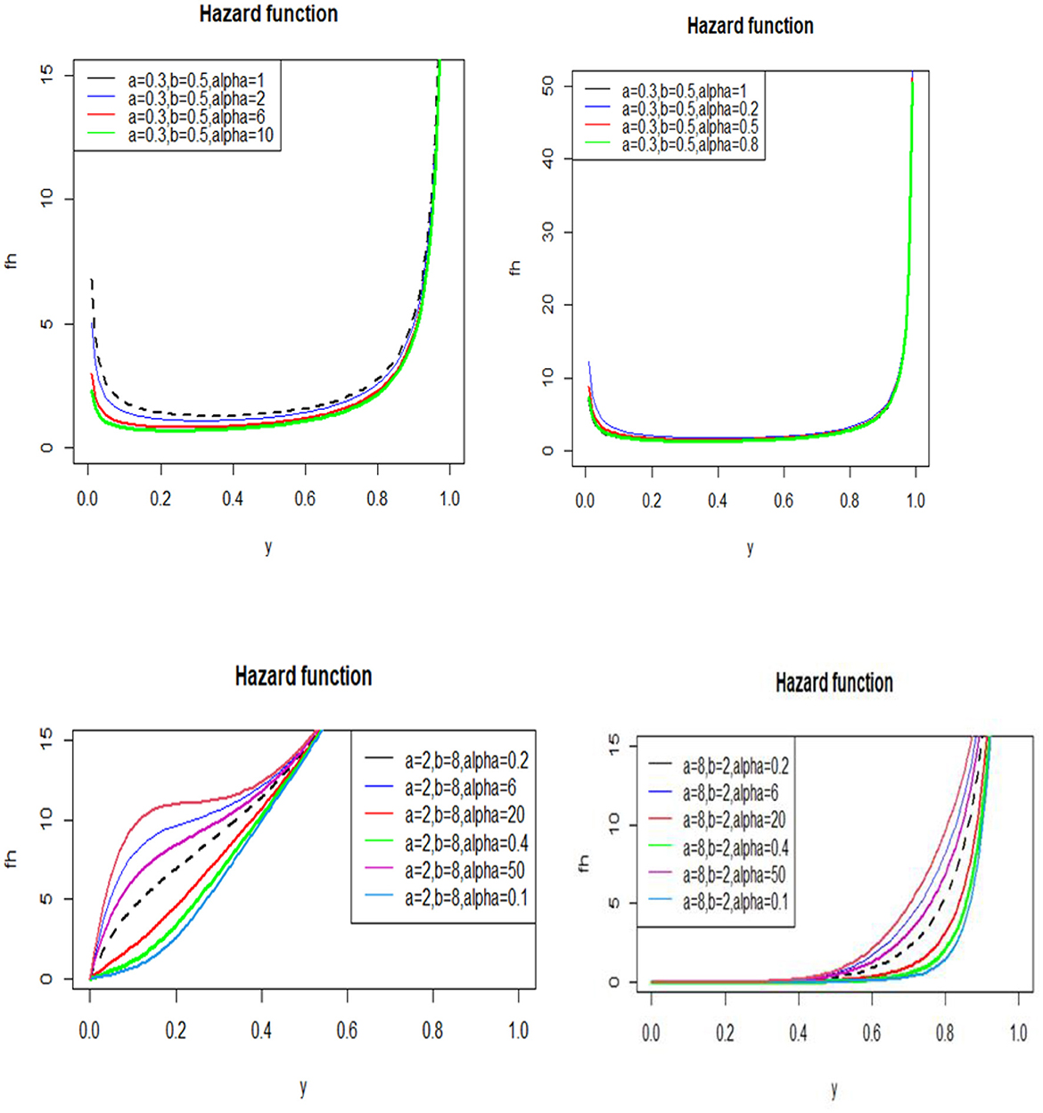
Figure 3. Hazard function plots for various values of the parameters a, b, and α.

6 Linear representation of the APT_Beta distribution

The PDF of Y has a linear representation for α > 0 and α ≠ 1 which is highly useful when deriving the statistical properties of generalized distributions and expanded using the power series as follows [20].

$\begin{array}{rr}{(\alpha )}^z={\displaystyle \sum _{k=0}^{\infty }}\frac{{(log(\alpha ))}^k}{k!}{z}^k& (16)\end{array}$

$\begin{array}{c}{(\alpha )}^{\frac{1}{B(a,b)}{\displaystyle {\int }_0^y}{x}^{a-1}{(1-x)}^{b-1}dx}={\displaystyle \sum _{k=0}^{\infty }}\frac{{(log(\alpha ))}^k}{k!}\\ {\left(\frac{1}{B(a,b)}{\displaystyle {\int }_0^y}{x}^{a-1}{(1-x)}^{b-1}dx\right)}^k\end{array}$

Thus the alpha power transformed beta distribution density can be linearly expressed as

$\begin{array}{ll}{f}_{APT}(y;a,b,\alpha )=\frac{log(\alpha )}{\alpha -1}{\displaystyle \sum _{k=0}^{\infty }}\frac{{(log(\alpha ))}^k}{k!}f(y){F(y)}^k& (17)\end{array}$

7 Properties of the APT_Beta distribution

This portion presents some important statistical characteristics of the APT_Beta distribution such as the mean residual life function, moment function shape measurments (skewness, kurtosis) and moment generating function.

7.1 Quantile function

Assume that Y ~APT_Beta (a,b,α); then the quantile function is given by

F(y) = M and we can solve explicitly for Y using the inverse of the CDF function

$\begin{array}{r}{F}^{-1}(Q(p))=y\\ F_{APT}(y;a,b,\alpha )=\frac{{(\alpha )}^{\frac{1}{B(a,b)}{\displaystyle {\int }_0^y}{x}^{a-1}{(1-x)}^{b-1}dx}-1}{\alpha -1}=Q(p)& (18)\end{array}$

where M is a random variable quantile function of the APT_Beta model and is given as

$\begin{array}{l}{B}_y(a,b)={\displaystyle {\int }_0^y}{x}^{a-1}{(1-x)}^{b-1}dx=B(a,b)\frac{log\left\{Q(p)(\alpha -1)+1\right\}}{log(\alpha )}\end{array}$

where B_y(a, b) is the incomplete beta function which according to Equation (21) can be expressed as an integer of Gauss hypergeometric function as follows

$\begin{array}{l}{B}_y(a,b)={\frac{y^a}{a}}_2{F}_1(a,1-b;a+1;y)\end{array}$

where ₂F₁(a, c; γ; y) = $\sum _{i=0}^{\infty }\frac{{(a)}_i{(b)}_i^{*}{y}^i}{{(\gamma )}_i^{*}i!}$

For mathematical simplification, the incomplete beta function and beta function ratio, which is the CDF of the beta distribution, can be expressed as a quantile function as follows:

$\begin{array}{l}{I}_y(a,b)=\frac{B_y(a,b)}{B(a,b)}=\frac{log\left\{Q(p)(\alpha -1)+1\right\}}{log(\alpha )}\end{array}$

Without this special case we cannot determine the quantile of Y explicitly due to the iinherent nature of the incomplete beta function.

7.2 Mean residual life function

The mean residual lifetime is the expected remaining lifespan of individuals at age t or the area of the survival curve to the right of time t divided by the survival function. Let the lifetime of an individual/object be represented by Y having an alpha power transformed beta distribution, then, the corresponding mean lifetime expression is

$\begin{array}{l}\mu (t)=\frac{{\displaystyle {\int }_0^{\infty }}(t-y)f(t)dt}{S(t)}=\frac{{\displaystyle {\int }_0^{\infty }}S(t)}{S(t)}=\frac{{\displaystyle {\int }_0^{\infty }}\frac{\alpha -{(\alpha )}^{I_y(a,b)}}{\alpha -1}dy}{\frac{\alpha -{(\alpha )}^{I_y(a,b)}}{\alpha -1}}\\ =\frac{{\displaystyle {\int }_0^{\infty }}\alpha -{\alpha }^{I_Y(a,b)}dy}{\alpha -{(\alpha )}^{I_Y(a,b)}}\\ \mu (t)=\frac{{\displaystyle {\int }_0^{\infty }}\alpha -{(\alpha )}^{\left[\frac{y^{a}2F1(a,1-b;1+a,y)}{aB(a,b)}\right]}dy}{\alpha -{\alpha }^{\left[\frac{y^{a}2F1(a,1-b;1+a,y)}{aB(a,b)}\right]}}& (19)\end{array}$

where 2F1(a, 1 − b; 1 + a, y) is the hypergeometric function.

7.3 Moment function

The moments of random variables correspond to the expected values of different powers. The first moment, also known as the expectation, holds significant importance in the field of probability and statistics. Additionally, the second moment, specifically the second central moment or variance, plays a crucial role in these domains.

Theorem 1: According to the definition of the r^th moment of Y, we have moments of the alpha power transformed beta distribution formulated by the principle of Equation 22 as for any r, a positive integer and if Y ∈ l^r, the r^th moment of Y is E(y^r).

$\begin{array}{r}E(y^r)={\displaystyle {\int }_0^1{y}^r}{f}_{APT}\left(y,a,b,\alpha \right)dy\\ E(y^r)=\frac{\ln (\alpha )}{(\alpha -1)}\frac{1}{B(a,b)}{\displaystyle {\int }_0^1\left({(\alpha )}^{{\displaystyle {\sum }_{k=0}^{b-1}{y}^{a+k}}}\right)}\\ {\displaystyle \sum _{k=0}^{b-1}\left(\frac{b-1}{k}\right)y^{a+r+k-1}}dy;if\alpha \ne 1& (20)\end{array}$

Proof

$\begin{array}{l}E(y^r)={\displaystyle {\int }_0^1{y}^r}\frac{\ln (\alpha )}{\alpha -1}\left({(\alpha )}^{\frac{1}{B(a,b)}{\displaystyle {\int }_0^y{x}^{a-1}{(1-x)}^{b-1}dx}}\right)\\ \frac{1}{B(a,b)}{y}^{a-1}{(1-y)}^{b-1}dy\\ E(y^r)={\displaystyle {\int }_0^1\frac{\ln (\alpha )}{\alpha -1}}\left({\alpha }^{I_Y(a,b)}\right)\frac{1}{B(a,b)}{y}^{a+r-1}{(1-y)}^{b-1}dy;\\ if\alpha \ne 1,a,b,\alpha >0,0<y<1\\ E(y^r)=\frac{\ln (\alpha )}{\alpha -1}\frac{1}{B(a,b)}{\displaystyle {\int }_0^1\left({(\alpha )}^{I_Y(a,b)}\right)y^{a+r-1}{(1-y)}^{b-1}dy};\\ if\alpha \ne 1,a,b,\alpha >0,0<y<1\\ E(y^r)=\frac{\ln (\alpha )}{(\alpha -1)}\frac{1}{B(a,b)}{\displaystyle {\int }_0^1\left({(\alpha )}^{{\displaystyle {\sum }_{k=0}^{b-1}{y}^{a+k}}}\right)y^{a+r-1}{(1-y)}^{b-1}dy};\\ if\alpha \ne 1,a,b,\alpha >0,0<y<1\end{array}$

where

$\begin{array}{c}{I}_Y(a,b)=\frac{1}{B(a,b)}{\displaystyle {\int }_0^y}{x}^{a-1}{(1-x)}^{b-1}dx\\ =\frac{{\displaystyle {\int }_0^y}{x}^{a-1}{\displaystyle {\sum }_{k=0}^{b-1}}(\frac{b-1}{k}){(1^{b-1-k})x}^{k}dy}{{\displaystyle {\int }_0^1}{y}^{a-1}{\displaystyle {\sum }_{k=0}^{b-1}}(\frac{b-1}{k}){(1^{b-1-k})y}^{k}dy}=\frac{{\displaystyle {\sum }_{k=0}^{b-1}}(\frac{b-1}{k}){{\displaystyle {\int }_0^y}x}^{a+k-1}dy}{{\displaystyle {\sum }_{k=0}^{b-1}}(\frac{b-1}{k}){\displaystyle {\int }_0^1}{y}^{a+k-1}dy}\\ =\frac{{\displaystyle {\sum }_{k=0}^{b-1}}(\frac{b-1}{k})\frac{y^{a+k}}{a+k}}{{\displaystyle {\sum }_{k=0}^{b-1}}(\frac{b-1}{k})\frac{1}{a+k}}={\displaystyle {\sum }_{k=0}^{b-1}}{y}^{a+k}\end{array}$

Therefore the moment becomes

$\begin{array}{l}E(y^r)=\frac{\ln (\alpha )}{(\alpha -1)}\frac{1}{B(a,b)}{\displaystyle {\int }_0^1\left({(\alpha )}^{{\displaystyle {\sum }_{k=0}^{b-1}{y}^{a+k}}}\right)}\\ {\displaystyle \sum _{k=0}^{b-1}\left(\frac{b-1}{k}\right)y^{a+r+k-1}}dy;if\alpha \ne 1 \end{array}$

Therefore, after some arithmetical employment, we have the desired proof.

Corollary 1. The mean of the alpha power transformed beta (APT_Beta) distribution computed for any y; If y ∈ l¹, where l¹ are all values in the interval integrable space, then the mean of y is E[y], the expectation of y [21] and formulated as follows:

$\begin{array}{l}E(y)=\frac{ln(\alpha )}{\alpha -1}\frac{1}{B(a,b)}{\displaystyle {\int }_0^1}({(\alpha )}^{{\displaystyle {\sum }_{k=0}^{b-1}}{y}^{a+k}}){\displaystyle {\sum }_{k=0}^{b-1}}(\frac{b-1}{k})y^{a+k}dy;\\ if\alpha \ne 1,0<y<1& (21)\end{array}$

Assuming that y ∈ l², where l² is the values integrable space, the variance of y is the second central moment:

$\begin{array}{l}var(y){=E\left[y^2\right]-\left[E(y)\right]}^2\end{array}$

To compute the variance in y that is distributed under the APT_Beta distribution, first, compute expectation of Y² as follows:

$\begin{array}{l}Var(y)=\frac{ln(\alpha )}{(\alpha -1)}\frac{1}{B(a,b)}{\displaystyle {\int }_0^1}({(\alpha )}^{{\displaystyle {\sum }_{k=0}^{b-1}}{y}^{a+k}}){\displaystyle {\sum }_{k=0}^{b-1}}(\frac{b-1}{k})y^{a+k+1}dy\\ -{\left[\frac{ln(\alpha )}{(\alpha -1)}\frac{1}{B(a,b)}{\displaystyle {\int }_0^1}({(\alpha )}^{{\displaystyle {\sum }_{k=0}^{b-1}}{y}^{a+k}}){\displaystyle {\sum }_{k=0}^{b-1}}(\frac{b-1}{k})y^{a+k}dy\right]}^2& (22)\end{array}$

Mode: A mode of the distribution of a r.v. Y is any point, if such points exist, that maximizes the probability density function of Y [34]. The mode is obtained by taking the first derivative of the probability density function.

Corollary 2: Let Y have the APT_Beta distribution, then the mode can be derived as follows.

$\begin{array}{r}\frac{\partial }{\partial y}{f}_{APT}(y,a,b,\alpha )=0\\ mode=\frac{\partial }{\partial y}\left[\frac{ln(\alpha )}{(\alpha -1)}({(\alpha )}^{I_y(a,b)})\frac{1}{B(a,b)}{y}^{a-1}{(1-y)}^{b-1}\right];\\ if\alpha \ne 1,0<y<1\end{array}$

Therefore the mode becomes

$\begin{array}{ll}Mode=\left[\frac{1}{\alpha -1}\right];if\alpha \ne 1,\alpha >0,0<y<1& (23)\end{array}$

Skewness

Skewness (the third central moment) represent the peakness of the distribution.

Corollary 3: assume that Y is distributed as an APT_Beta distribution; hence, the skewness can be expressed as

$\begin{array}{l}{\mu }_3={E(y-E(y))}^3=E(y^3)-3E(y^2)E(y)+2{\left[E(y)\right]}^3\\ {\mu }_3=\frac{ln(\alpha )}{(\alpha -1)}\frac{1}{B(a,b)}{\displaystyle {\int }_0^1}({(\alpha )}^{I_y(a,b)})y^{a+2}{(1-y)}^{b-1}dy\\ -3\frac{ln(\alpha )}{(\alpha -1)}\frac{1}{B(a,b)}{\displaystyle {\int }_0^1}({\alpha }^{I_y(a,b)})y^{a+1}{(1-y)}^{b-1}dy\\ \left[\frac{ln(\alpha )}{(\alpha -1)}\frac{1}{B(a,b)}{\displaystyle {\int }_0^1}({\alpha }^{I_y(a,b)})y^a{(1-y)}^{b-1}dy\right]\\ +2{\left[\frac{ln(\alpha )}{(\alpha -1)}\frac{1}{B(a,b)}{\displaystyle {\int }_0^1}({\alpha }^{I_y(a,b)})y^a{(1-y)}^{b-1}dy\right]}^3& (24)\end{array}$

Kurtosis

Kurtosis can be expressed as

$\begin{array}{l}{\mu }_4=E\left(y^4\right)-4E\left(y^3\right)E\left(y\right)+6{\left[E\left(y\right)\right]}^{2}E\left(y^2\right)-3{\left[E\left(y\right)\right]}^4\\ {\mu }_4=\frac{\ln (\alpha )}{(\alpha -1)}\frac{1}{B(a,b)}{\displaystyle {\int }_0^1\left({(\alpha )}^{I_y(a,b)}\right)}{y}^{a+3}{(1-y)}^{b-1}dy\\ -4\frac{\ln \left(\alpha \right)}{\left(\alpha -1\right)}\frac{1}{B\left(a,b\right)}{\displaystyle {\int }_0^1\left({\left(\alpha \right)}^{I_y\left(a,b\right)}\right)}{y}^{a+2}{\left(1-y\right)}^{b-1}dy\\ \left[\frac{\ln \left(\alpha \right)}{\left(\alpha -1\right)}\frac{1}{B\left(a,b\right)}{\displaystyle {\int }_0^1\left({\left(\alpha \right)}^{I_y\left(a,b\right)}\right)y^a{\left(1-y\right)}^{b-1}dy}\right]\\ +6{\left[\frac{\ln \left(\alpha \right)}{\left(\alpha -1\right)}\frac{1}{B\left(a,b\right)}{\displaystyle {\int }_0^1\left({\alpha }^{I_y\left(a,b\right)}\right)y^a{\left(1-y\right)}^{b-1}dy}\right]}^2\\ \left(\frac{\ln \left(\alpha \right)}{\left(\alpha -1\right)}\frac{1}{B\left(a,b\right)}{\displaystyle {\int }_0^1\left({\alpha }^{I_y\left(a,b\right)}\right)y^{a+1}{\left(1-y\right)}^{b-1}dy}\right)\\ -3{\left[\frac{\ln \left(\alpha \right)}{\left(\alpha -1\right)}\frac{1}{B\left(a,b\right)}{\displaystyle {\int }_0^1\left({(\alpha )}^{I_y\left(\gamma ,b\right)}\right)y^{\gamma }{\left(1-y\right)}^{b-1}dy}\right]}^4& (25)\end{array}$

7.4 Moment generation

The moment generating function of Y is the function Φ_y(t) = E[e^ty], provided that the expectation exists for all t in some neighborhood of the origin (Equation 22). The moment-generating function of random variable Y that follows the alpha power transformed beta (APT_beta) distribution, if it exists, is given by:

$\begin{array}{c}{\Phi }_y\left(t\right)=E\left(e^{yt}\right)={\displaystyle {\int }_0^{\infty }}{e}^{yt}\frac{ln\left(\alpha \right)}{\alpha -1}\left({\left(\alpha \right)}^{\frac{1}{B\left(a,b\right)}{\displaystyle {\int }_0^y}{x}^{a-1}{\left(1-x\right)}^{b-1}dx}\right)\\ \frac{1}{B\left(a,b\right)}{y}^{a-1}{\left(1-y\right)}^{b-1}dy\\ {\Phi }_y\left(t\right)=E\left(e^{yt}\right)=\frac{ln\left(\alpha \right)}{\left(\alpha -1\right)}\\ \frac{1}{B\left(a,b\right)}{\displaystyle {\int }_0^{\infty }}{e}^{yt}\left({\left(\alpha \right)}^{\frac{1}{B\left(a,b\right)}{\displaystyle {\int }_0^y}{x}^{a-1}{\left(1-x\right)}^{b-1}dx}\right)\\ y^{a-1}{\left(1-y\right)}^{b-1}dy\\ {\Phi }_y\left(t\right)=\frac{ln\left(\alpha \right)}{\left(\alpha -1\right)}{\displaystyle {\int }_0^1}\left({\alpha }^{I_y\left(a,b\right)}\right)\frac{1}{B\left(a,b\right)}{y}^{a-1}{\left(1-y\right)}^{b-1}{e}^{yt}dy& (26)\end{array}$

8 Classical estimation

Classical estimation uses the maximum likelihood principle to estimate population parameters from a sample in research and data analysis.

8.1 Maximum likelihood estimation

Maximum Likelihood Estimation (MLE) is a powerful technique for estimating unknown parameters by maximizing the likelihood of observed data. MLE, assuming independent and identically distributed (i.i.d.) observations, provides efficient estimation based on unbiasedness and minimum variance criteria [34].

Let Y₁, Y₂, . . . , Y_n is an independent identically distributed random variable with an alpha Power transformed beta distribution $f_{APT}$(^.; θ), θϵΩ⊆R and consider the joint pdf of Y's f_APT(Y₁; θ)……….f_APT(Y_n; θ); then, the likelihood function is given by

$\begin{array}{r}L\left(Y,a,b,\alpha \right)={\left(\frac{ln\left(\alpha \right)}{\left(\alpha -1\right)\left(B\left(a,b\right)\right)}\right)}^n{\displaystyle \prod _{i=1}^n}\left({\left(\alpha \right)}^{I_y\left(a,b\right)}\right)y^{a-1}\\ {\displaystyle \prod _{i=1}^n}{\left(1-y\right)}^{b-1}& (27)\end{array}$

The estimates $\widehat{\theta }=\widehat{\theta }(Y_1$,Y₂, . . . , Y_n) is called the maximum likelihood estimate of θ if

$\begin{array}{l}L(\widehat{\theta }|Y_1,Y_2,\mathrm{...},Y_n)=max(L\left(\theta |Y_1,Y_2,...,Y_n\right);\\ \theta \epsilon \Omega )\end{array}$

[34]

where θ = (a, b, α) and $\widehat{\theta }=(â,\widehat{b},\widehat{\alpha })$.

The log-likelihood function of L(a, b, α) is given by

$\begin{array}{c}loglik(y,a,b,\alpha )=ll=nln(ln(\alpha ))-nln(\alpha -1)-nln(B(a,b))\\ +ln(\alpha ){\displaystyle {\sum }_{i=1}^n}{I}_y(a,b)+(a-1){\displaystyle {\sum }_{i=1}^n}ln(y_i)\\ +(b-1){\displaystyle {\sum }_{i=1}^n}ln(1-y_i)& (28)\end{array}$

Then, we can take the first derivative of the log likelihood function with respect to each parameter as follows.

$\begin{array}{ll}\frac{\partial ll}{\partial \alpha }=\frac{n}{ln\left(\alpha \right)}\left(\frac{1}{\alpha }\right)-\frac{n}{\alpha -1}+\frac{{\displaystyle {\sum }_{i=1}^n}{I}_y\left(a,b\right)}{\alpha }=0& (29)\end{array}$

$\begin{array}{r}\frac{\partial ll}{\partial a}=\frac{-n}{B\left(a,b\right)}\frac{\partial }{\partial a}B\left(a,b\right)+ln\left(\alpha \right){\displaystyle \sum _{i=1}^n}\frac{d{I}_y\left(a,b\right)}{da}\\ +{\displaystyle \sum _{i=1}^n}ln\left(y_i\right)=0& (30)\end{array}$

$\begin{array}{c}\frac{\partial ll}{\partial b}=\frac{-n}{B\left(a,b\right)}\frac{\partial }{\partial b}B\left(a,b\right)+ln\left(\alpha \right){\displaystyle {\sum }_{i=1}^n}\frac{d{I}_y\left(a,b\right)}{db}\\ +{\displaystyle {\sum }_{i=1}^n}ln\left(1-y_i\right)=0& (31)\end{array}$

Let $derivativeof-\frac{\partial }{\partial a}ln(B(a,b))$ become (ψ⁰(a + b) − ψ⁰(a))

That is $-\frac{\partial }{\partial a}ln(B(a,b))=-\frac{\partial }{\partial a}ln\left(\frac{\Gamma (a)\Gamma (b)}{\Gamma (a+b)}\right)=-\frac{\partial }{\partial a}(ln(\Gamma (a))+ln(\Gamma (b))-ln(\Gamma (a+b)))=-\left(\frac{{\Gamma }^{\prime }(a)}{\Gamma (a)}-\frac{{\Gamma }^{\prime }(a+b)}{\Gamma (a+b)}\right)=\left({\psi }^0(a+b)-{\psi }^0(a)\right)$

then Equation 30 and 31 become

$\begin{array}{c}\frac{\partial ll}{\partial a}=n({\psi }^0(a+b)-{\psi }^0(a))+ln(\alpha ){\displaystyle {\sum }_{i=1}^n}\frac{d{I}_y(a,b)}{da}\\ +{\displaystyle {\sum }_{i=1}^n}ln(y_i)=0& (32)\end{array}$

$\begin{array}{c}\frac{\partial ll}{\partial b}=n({\psi }^0(a+b)-{\psi }^0(b))+ln(\alpha ){\displaystyle {\sum }_{i=1}^n}\frac{d{I}_y(a,b)}{db}\\ +{\displaystyle {\sum }_{i=1}^n}ln(1-y_i)=0& (33)\end{array}$

After this second derivative is applied, the Newton–Raphson method can be used to solve non-linear equations and find the unknown parameters.

8.2 Asyptotic confidence interval

Constructing an estimator on the basis of a sample of fixed size n is possible in maximum likelihood function. However, as the sample size n may increase indefinitely and produce sequence of estimators, the asymptotic distribution of the MLEs becomes:

$\begin{array}{l}\left[\left(â-a\right),\left(\widehat{b}-b\right),\left(\widehat{\alpha }-\alpha \right)\right]\to N\left(0,cov\left(â,\widehat{b},\widehat{\alpha }\right)\right)\end{array}$

where $cov(â,\widehat{b},\widehat{\alpha })$ are the variance covariance matrices of the estimators of parameters a, b, and α which can be approximated by the inverse of the observed Fisher-information matrix [34]. The observed Fisher-information matrix is given by

$\begin{array}{l}I\left(â,\widehat{b},\widehat{\alpha }\right)=\left(\begin{array}{c}\frac{{\partial }^{2}ll}{\partial a^2}\frac{{\partial }^{2}ll}{\partial a\partial b}\frac{{\partial }^{2}ll}{\partial a\partial \alpha }\\ \frac{{\partial }^{2}ll}{\partial b\partial a}\frac{{\partial }^{2}ll}{\partial b^2}\frac{{\partial }^{2}ll}{\partial b\partial \alpha }\\ \frac{{\partial }^{2}ll}{\partial \alpha \partial a}\frac{{\partial }^{2}ll}{\partial \alpha \partial b}\frac{{\partial }^{2}ll}{\partial {\alpha }^2}\\ \\ \end{array}\right)\end{array}$

where

$\begin{array}{r}\frac{{\partial }^{2}l}{\partial a^2}=n\left({\psi }^1\left(a+b\right)-{\psi }^1\left(a\right)\right)+ln\left(\alpha \right){\displaystyle \sum _{i=1}^n}\frac{{\partial }^2{I}_y\left(a,b\right)}{\partial a^2}\\ \frac{{\partial }^{2}l}{\partial a\partial b}=n\left({\psi }^1\left(a+b\right)\right)+ln\left(\alpha \right){\displaystyle \sum _{i=1}^n}\frac{{\partial }^2{I}_y\left(a,b\right)}{\partial a\partial b}\\ \frac{{\partial }^{2}l}{\partial b^2}=n\left({\psi }^1\left(a+b\right)-{\psi }^1\left(b\right)\right)+ln\left(\alpha \right){\displaystyle \sum _{i=1}^n}\frac{{\partial }^2{I}_y\left(a,b\right)}{\partial b^2}\\ \frac{{\partial }^{2}l}{\partial {\alpha }^2}=\left(\frac{n}{{\alpha }^2{\left(ln\alpha \right)}^2}-\frac{1}{{\alpha }^{2}ln\left(\alpha \right)}\right)+\frac{n}{{\left(\alpha -1\right)}^2}-\frac{{\displaystyle {\sum }_{i=1}^n}{I}_y\left(a,b\right)}{{\alpha }^2}\\ \frac{{\partial }^{2}l}{\partial a\partial \alpha }=\frac{1}{\alpha }{\displaystyle \sum _{i=1}^n}\frac{\partial I_y\left(a,b\right)}{\partial a}\\ \frac{{\partial }^{2}l}{\partial b\partial \alpha }=\frac{1}{\alpha }{\displaystyle \sum _{i=1}^n}\frac{\partial I_y\left(a,b\right)}{\partial b}\end{array}$

Then, the approximate 100(1 – γ)% two-sided confidence intervals for a, b and α are, given by

$\begin{array}{ll}â\pm Z_{\gamma /2}^{*}\sqrt{{I^{-1}}_{11}\left(â\right)},\widehat{b}\pm Z_{\frac{\gamma }{2}}^{*}\sqrt{{I^{-1}}_{22}\left(\widehat{b}\right)},\widehat{\alpha }\pm Z_{\gamma /2}^{*}\sqrt{{I^{-1}}_{33}\left(\widehat{\alpha }\right)}& (34)\end{array}$

where Z_γ/2 is the upper 100^th (γ/2) percentile of the standard normal distribution.

9 Order statistics

Assume that X₁, …., X_n are i.i.d random variables from the cumulative distribution F(x). Then Y₁ ≤ … ≤ Y_n where Y are the X_i arranged in order of increasing magnitude are called order statistics [34]. Let Y ≤ … ≤ Y_n be random samples in order statistics obtained from the alpha power transformed beta distribution then the marginal cumulative probability distribution function of Y_i is given by

$\begin{array}{r}{F}_{{APTy}_i}\left(y\right)={\displaystyle \sum _{j=i}^n}\left(\frac{n}{j}\right){\left[F\left(y\right)\right]}^j{\left[1-F\left(y\right)\right]}^{n-j}\\ F_{{APTy}_i}\left(y\right)={\displaystyle \sum _{j=i}^n}\left(\frac{n}{j}\right){\left[\frac{{\alpha }^{\frac{1}{B\left(a,b\right)}{\displaystyle {\int }_0^y}{x}^{a-1}{\left(1-x\right)}^{b-1}dx}-1}{\alpha -1}\right]}^j\\ {\left[1-\left(\frac{{\left(\alpha \right)}^{\frac{1}{B\left(a,b\right)}{\displaystyle {\int }_0^y}{x}^{\alpha -1}{\left(1-x\right)}^{b-1}dx}-1}{\alpha -1}\right)\right]}^{n-j}\\ F_{APT{y}_i}\left(y\right)={\displaystyle \sum _{j=i}^n}\left(\frac{n}{j}\right){\left[\frac{{\left(\alpha \right)}^{\frac{1}{B\left(a,b\right)}{\displaystyle {\int }_0^y}{x}^{a-1}{\left(1-x\right)}^{b-1}dx}-1}{\alpha -1}\right]}^j\\ {\left[\frac{{\alpha -\left(\alpha \right)}^{\frac{1}{B\left(a,b\right)}{\displaystyle {\int }_0^y}{x}^{a-1}{\left(1-x\right)}^{b-1}dx}}{\alpha -1}\right]}^{n-j}& (35)\end{array}$

The corresponding alpha power transformed beta probability density function can be given by

$\begin{array}{r}{f_{APT}}_{y_i}\left(y\right)=\frac{n!}{\left(i-1\right)\left(n-i\right)}{\left[F\left(y\right)\right]}^{i-1}{\left[1-F\left(y\right)\right]}^{n-i}{f}_{APT}\left(y\right)\\ {f_{APT}}_{y_i}\left(y\right)=\frac{n!}{\left(i-1\right)!\left(n-i\right)!}{\left[\frac{{\left(\alpha \right)}^{\frac{1}{B\left(a,b\right)}{\displaystyle {\int }_0^y}{x}^{a-1}{\left(1-x\right)}^{b-1}dx}-1}{\alpha -1}\right]}^{i-1}\\ {\left[1-\left(\frac{{\left(\alpha \right)}^{\frac{1}{B\left(a,b\right)}{\displaystyle {\int }_0^y}{x}^{a-1}{\left(1-x\right)}^{b-1}dx}-1}{\alpha -1}\right)\right]}^{n-i}\\ \frac{ln\left(\alpha \right)}{\alpha -1}\left({\left(\alpha \right)}^{\frac{1}{B\left(a,b\right)}{\displaystyle {\int }_0^y}{x}^{a-1}{\left(1-x\right)}^{b-1}dx}\right)\frac{1}{B\left(a,b\right)}{y}^{a-1}{\left(1-y\right)}^{b-1}\\ {f_{APT}}_{y_i}\left(y\right)=\frac{n!}{\left(i-1\right)!\left(n-i\right)!}\\ \frac{ln\left(\alpha \right)}{\alpha -1}\left({\left(\alpha \right)}^{\frac{1}{B\left(a,b\right)}{\displaystyle {\int }_0^y}{x}^{a-1}{\left(1-x\right)}^{b-1}dx}\right)\frac{1}{B\left(a,b\right)}{y}^{a-1}{\left(1-y\right)}^{b-1}\\ {\left[\frac{{\left(\alpha \right)}^{\frac{1}{B\left(a,b\right)}{\displaystyle {\int }_0^y}{x}^{a-1}{\left(1-x\right)}^{b-1}dx}-1}{\alpha -1}\right]}^{i-1}\\ {\left[1-\left(\frac{{\left(\alpha \right)}^{\frac{1}{B\left(a,b\right)}{\displaystyle {\int }_0^y}{x}^{a-1}{\left(1-x\right)}^{b-1}dx}-1}{\alpha -1}\right)\right]}^{n-i}& (36)\end{array}$

If X₁X1, . . . , X_n are i.i.d. r.v.'s with APT_Beta p.d.f which is positive for 0 < x < 1 and 0 otherwise, then the joint p.d.f. of the order statistics Y₁, . . . , Y_n is given by:

$\begin{array}{ll}G\left(Y_1,...,Y_n\right)=\{\begin{array}{c}n!f_{APT}\left(y_1\right)\dots ..f_{APT}\left(y_n\right)\\ 0otherwise\end{array}& (37)\end{array}$

10 Simulation of APT_Beta distribution using AR sampling

The simulation aims to assess the performance of the APT_Beta distribution by evaluating its pdf, cdf, and probabilistic axioms using random data. Maximum likelihood estimation parameters are tested for flexibility and performance through computation of mean square error (MSE), Mean Absolute Error (MAE), and Mean Absolute Percentage Error (MAPE) across various sample sizes and specific distribution parameters true value. The simulation, conducted in R programming, involves different values of alpha and other parameters using the acceptance-rejection algorithm concept [22].

The APT_Beta distribution was analyzed with parameters assigned values from three selected sets. Using the Newton-Raphson optimum algorithm technique in R programming, average estimates and error metrics like MSE, MAE, and MAPE were computed for MLE across various sample sizes in simulation data [23].

The MSE is determined by adding the variance of the estimate from the inverse Hessian matrix diagonal to the square of the bias from Maximum Likelihood Estimation (MLE) [34]. MAE and MAPE are calculated based on bias for each parameter, serving as measures of accuracy and consistency in parameter estimation [24]. According to the findings presented in Table 1 as sample size increases, MSE, MAE, and MAPE for MLE are expected to decrease, indicating more accurate and reliable estimates with larger sample sizes. For parameters, increasing sample size leads to decreasing MSEs and convergence of estimated values to true values.

Table 1

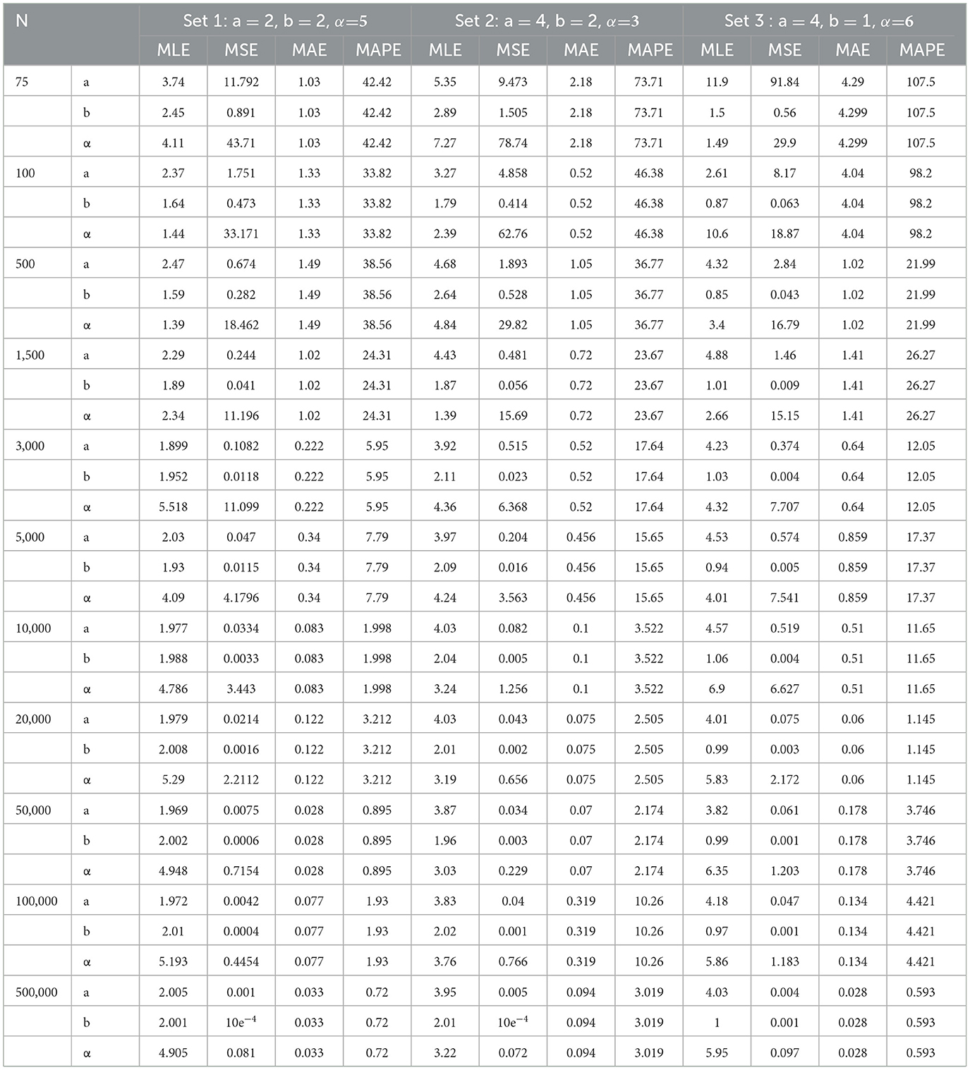
Table 1. MLE of the parametrs for different true values from the simulation.

11 Real data application

This study utilized the APT_Beta distribution to analyze prenatal care visit proportions from the Mini EDHS-2019 dataset. Parameters were estimated using MLE in natural logarithm form, with results transformed for maximization. Data on ANC visits were converted to proportions, focusing on a subset of 227 women in Addis Ababa who had undergone antenatal care visits.

Additionally, a second set of real data consists of 50 burr observations (measured in millimeters). The hole diameter is 12 mm, and the sheet thickness is 3.15 mm. These measurements were taken from a single machine introduced by Dasgupta [25]. The observation list is 0.04, 0.02, 0.06, 0.12, 0.14, 0.08, 0.22, 0.12, 0.08, 0.26, 0.24, 0.04, 0.14, 0.16, 0.08, 0.26, 0.32, 0.28, 0.14, 0.16, 0.24, 0.22, 0.12, 0.18, 0.24, 0.32, 0.16, 0.14, 0.08, 0.16, 0.24, 0.16, 0.32, 0.18, 0.24, 0.22, 0.16, 0.12, 0.24, 0.06, 0.02, 0.18, 0.22, 0.14, 0.06, 0.04, 0.14, 0.26, 0.18, 0.16.

Various model selection criteria like AIC [26], CAIC, BIC [27], Kolmogorov-Smirnov (K-S) [28], and HQIC [29] are used to compare statistical models, aiming to find the best fit. These criteria help compare distributions like APT-Beta, Weibull, exponential Weibull, Kumaraswamy Beta, and beta distributions. The model with the smallest absolute value for AIC, CAIC, BIC, and HQIC is considered the best, prioritizing a balance between goodness of fit and model complexity. A smaller (more negative) value indicates a preferable model over one with a larger (less negative) value.

Table 2's results offer further evidence supporting the notion that the suggested APT_Beta distribution outperforms the Weibull, Kumaraswamy Beta, and Beta distributions. according to these data, APT_Beta exhibited a similar effect to Exponential Weibull.

Table 2

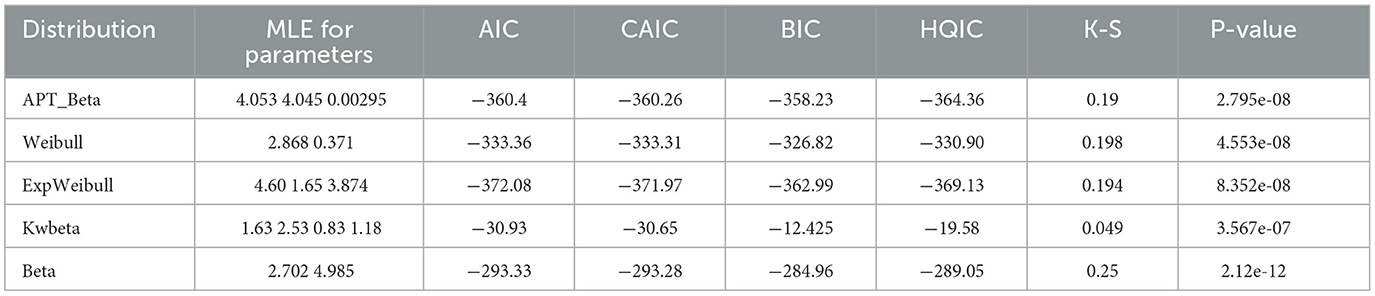
Table 2. Goodness of fit test tesults for ANC dataset.

Table 3 provides conclusive evidence supporting the similarity of the newly proposed distribution to the included distributions, with the exception of the beta distribution, for the provided data. The APT-Beta distribution surpasses the basic beta distribution in terms of effectiveness.

Table 3

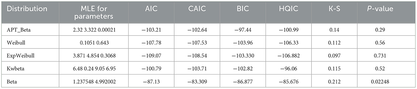
Table 3. Goodness of fit test results for burr dataset.

12 Discussion

Probability distributions are essential in statistical analysis for modeling real-world data. While the basic beta distribution is versatile, a new distribution called the alpha power transformed beta (APT_Beta) distribution aims to enhance flexibility and accuracy. By integrating additional parameters, the APT-Beta distribution overcomes limitations of the basic beta distribution, providing a more adaptable model for a wider range of outcomes and improved depiction of real-world scenarios.

The APT-Beta distribution excels in fitting observed data, outperforming other beta family models and offering versatility in modeling hazard rates. Its adaptability to real-world data, such as maternal antenatal care proportions and other proportions, makes it a preferred choice for researchers and practitioners seeking accurate representation and analysis of empirical data.

13 Conclusion

In statistics, modeling distributions is crucial for analyzing real-world data. The APT_Beta distribution, a three-parameter model introduced in this study, offers tractability, efficiency, and versatility for modeling bounded data. Constructed using the alpha power transformation approach, it provides a flexible and robust model for accurately capturing various types of bounded data in different applications.

The APT_Beta distribution is advantageous due to its tractability, allowing for easy derivation and analysis of mathematical properties. It demonstrates excellent performance in fitting real-world data with bounded characteristics, outperforming other distributions in goodness-of-fit measures. Its versatility, with three parameters accommodating a wide range of shapes, makes it a superior choice for modeling bounded data in diverse fields like finance, biology, and engineering. Apart from its versatility, the APT_Beta distribution also offers practical benefits in terms of efficiency. The distribution can be easily estimated using maximum likelihood estimation techniques, and the estimation process is computationally efficient. This allows for quick and accurate parameter estimation, even when dealing with large datasets.

The simulation study assessed the APT_Beta distribution's validity and parameter consistency with different sample sizes, and also using real-life data from Addis Ababa city and the burr dataset the validity and parameter consistency were examined. Results show its flexibility and effectiveness in modeling bounded data, making it a valuable tool for various disciplines like reliability engineering, medicine, economics, and life sciences. The APT_Beta distribution's alpha power transformation from the basic beta distribution offers versatility and efficiency in statistical modeling tasks, proving beneficial for researchers and practitioners in diverse fields.

Data availability statement

The datasets presented in this study can be found in online repositories. The names of the repository/repositories and accession number(s) can be found in the article/Supplementary material.

Author contributions

AA: Data curation, Formal analysis, Investigation, Methodology, Project administration, Software, Visualization, Writing – original draft, Writing – review & editing. AG: Project administration, Software, Supervision, Validation, Writing – review & editing. BA: Supervision, Validation, Visualization, Writing – review & editing.

Funding

The author(s) declare that no financial support was received for the research, authorship, and/or publication of this article.

Conflict of interest

The authors declare that the research was conducted in the absence of any commercial or financial relationships that could be construed as a potential conflict of interest.

Publisher's note

All claims expressed in this article are solely those of the authors and do not necessarily represent those of their affiliated organizations, or those of the publisher, the editors and the reviewers. Any product that may be evaluated in this article, or claim that may be made by its manufacturer, is not guaranteed or endorsed by the publisher.

Supplementary material

The Supplementary Material for this article can be found online at: https://www.frontiersin.org/articles/10.3389/fams.2024.1433767/full#supplementary-material

References

1. Alshkaki RSA. A six parameters beta distribution with application for modeling waiting time of muslim early morning prayer. In: Annals of Data Science. Springer Berlin Heidelberg (2021). doi: 10.1007/s40745-020-00282-0

Crossref Full Text | Google Scholar

2. Ng DW, Koh SK, Sim SZ, Lee MC. The study of properties on generalized Beta distribution. in Journal of Physics: Conference Series. IOP Publishing (2018). p. 012080. doi: 10.1088/1742-6596/1132/1/012080

Crossref Full Text | Google Scholar

3. Trenkler G. Continuous univariate distributions. In: Computational Statistics and Data Analysis (1996). doi: 10.1016/0167-9473(96)90015-8

Crossref Full Text | Google Scholar

4. Silva RB, Barreto-Souza W, Cordeiro GM. A new distribution with decreasing, increasing and upside-down bathtub failure rate. Comput Stat Data An. (2010) 54:935–44. doi: 10.1016/j.csda.2009.10.006

PubMed Abstract | Crossref Full Text | Google Scholar

5. Cordeiro GM, Silva RB, Nascimento AD. Recent Advances in Lifetime and Reliability Models. Sharjah: Bentham Science Publishers. (2020). doi: 10.2174/97816810834521200101

Crossref Full Text | Google Scholar

6. Aljarrah MA, Lee C, Famoye F. On generating tx-family of distributions using quantile functions. J Stat Distr Applic. (2014) 1:1–17. doi: 10.1186/2195-5832-1-2

Crossref Full Text | Google Scholar

7. Al-Aqtash R, Famoye F, Lee C. On generating a new family of distributions using the logit function. J Prob Stat Sci. (2015) 13:135–52.

Google Scholar

8. Cordeiro GM, Alizadeh M, Ramires TG, Ortega EM. The generalized odd half-Cauchy family of distributions: Properties and applications. Commun Stat Theory Methods. (2017) 46:5685–705. doi: 10.1080/03610926.2015.1109665

Crossref Full Text | Google Scholar

9. Almarashi M, Elgarhy M. A new muth generated family of distributions with applications. J Nonlinear Sci Applic. (2018) 11:1171–84. doi: 10.22436/jnsa.011.10.06

Crossref Full Text | Google Scholar

10. Mahdavi A, Kundu D. A new method for generating distributions with an application to exponential distribution. Commun Stat Theory Methods. (2017) 46:6543–57. doi: 10.1080/03610926.2015.1130839

Crossref Full Text | Google Scholar

11. Chotikapanich D, Rao DSP, Tang KK. Estimating income inequality in china using grouped data and the generalized beta distribution. In: Review of Income and Wealth. Wiley: Hoboken, NY, USA (2007). p. 127–147. doi: 10.1111/j.1475-4991.2007.00220.x

Crossref Full Text | Google Scholar

12. McDonald JB, Richards DO. Hazard rates and generalized beta distributions. IEEE Trans. Reliab. (1987) 36:463–6. doi: 10.1109/TR.1987.5222439

Crossref Full Text | Google Scholar

13. Libby DL, Novick MR. Multivariate generalized beta distributions with applications to utility assessment. J Educ Statist. (1982) 7:271–94. doi: 10.3102/10769986007004271

PubMed Abstract | Crossref Full Text | Google Scholar

14. Allendoerfer C, Oakley C, Kerr D. Elementary Functions. New York: McGraw-Hill, Inc. (1977).

Google Scholar

15. Mathews D, Brown P, Evans M. Supporting Australian Mathematics Project Polynomial Function. (2013).

Google Scholar

16. Bourguignon M, Silva R, Cordeiro G. The weibull-G family of probability distributions. J Data Sci. (2014) 12:53–68. doi: 10.6339/JDS.201401_12(1).0004

Crossref Full Text | Google Scholar

17. Robert CP. The Bayesian Choice From Decision-Theoretic Foundations to Computational Implementation. 2^nd Edition, New York: Springer Science+Business Media, LLC. (2007).

Google Scholar

18. Lawless J. Statistical Models and Methods for Lifetime Data, ser. Wiley Series in Probability and Statistics. London: Wiley. (2011).

Google Scholar

19. Moore DF. Applied Survival Analysis Using R. Rutgers School of Public Health. Piscataway, NJ, USA, Springer (2016).

Google Scholar

20. Olver F, Lozier D. NIST Handbook of Mathematical Functions. Cambridge: Cambridge University Press (2010).

Google Scholar

21. Karr AF. Probability. New York: Springer Science+Business Media, LLC. (1992).

Google Scholar

22. Casella G, Robert CP, Wells MT. Lecture Notes-Monograph Series. (2015). p. 342–347.

Google Scholar

23. Henningsen A, Toomet O. maxLik: a package for maximum likelihood estimation in R. Comput Stat. (2011) 26:443–58. doi: 10.1007/s00180-010-0217-1

PubMed Abstract | Crossref Full Text | Google Scholar

24. Vandeput N. Choosing the Right Forecasting Metric is not Straightforward. Let's Review the Pro and con of RMSE, MAE, MAPE, and Bias. (2019).

PubMed Abstract | Google Scholar

25. Dasgupta R. On the distribution of burr with applications. Sankhya B. (2011) 73:1–19. doi: 10.1007/s13571-011-0015-y

Crossref Full Text | Google Scholar

26. Akaike H. Information theory and an extension of the maximum likelihood principle. In: Selected Papers of hirotugu akaike. New York, NY: Springer New York (1973). p. 199–213. doi: 10.1007/978-1-4612-1694-0_15

Crossref Full Text | Google Scholar

27. Schwarz G. Estimating the dimension of a model. Ann Stat. (1978) 6:461–4. doi: 10.1214/aos/1176344136

PubMed Abstract | Crossref Full Text | Google Scholar

28. Kolmogorov AN. On the Empirical Determination of a Distribution Function. Giornale dell'Instituto Italiano degli Attuari. (1933) 4:83–91.

Google Scholar

29. Hannan EJ, Quinn BG. The determination of the order of an autoregression. J R Stat Soc B. (1979) 41:190–5. doi: 10.1111/j.2517-6161.1979.tb01072.x

Crossref Full Text | Google Scholar

30. Marshall AW, Olkin I. A new method for adding a parameter to a family of distributions with application to the exponential and weibull families. Biometrika. (1997) 84:641–52. doi: 10.1093/biomet/84.3.641

Crossref Full Text | Google Scholar

31. Jammalamadaka SR, Bury K. Statistical Distributions in Engineering. Cambridge University Press (2000). doi: 10.2307/2685598

Crossref Full Text | Google Scholar

32. Gupta RC, Gupta PL, Gupta RD. Modeling failure time data by Lehman alternatives. Commun Stat Theor Methods. (1998) 27:887–904.

PubMed Abstract | Google Scholar

33. Exton H. Multiple Hypergeometric Functions and Applications. Chichester; New York, NY: Ellis Horwood (1976).

Google Scholar

34. Roussas G. A Course in Mathematical Statistics. 2nd ed. Academic Press (1997).

Google Scholar

35. Khalil A, Ahmadini AAH, Ali M, Mashwani WK, Alshqaq SS, Salleh Z, et al. A novel method for developing efficient probability distributions with applications to engineering and lifescience data. Hindawi J Math. (2021) 2021:4479270.

Google Scholar

36. Baharith LA, Aljuhani WH. New method for generating new families of distributions. Symmetry. (2021) 13:726. doi: 10.3390/sym13040726

Crossref Full Text | Google Scholar

37. Rainville ED. Special Functions. New York, NY: Macmillan (1960).

Google Scholar