 Karl Schweizer
 Xuezhu Ren
 Tengfei Wang
95% of researchers rate our articles as excellent or good
Learn more about the work of our research integrity team to safeguard the quality of each article we publish.
Find out more
METHODS article
Front. Appl. Math. Stat. , 23 August 2024
Sec. Statistics and Probability
Volume 10 - 2024 | https://doi.org/10.3389/fams.2024.1423726
Estimates of factor variances observed together with negative factor correlations in CFA using the bifactor model are explored for specific characteristics. The analysis is conducted on the basis of quantified accounts of common systematic variation achieved by the two group latent variables of the model. It reveals that negative factor correlations tend to be associated with larger factor variance estimates than the zero correlation and positive correlations. Further, it reveals that upper limits to the sizes of factor variances for positive factor correlations corresponding to expectations exist while in negative correlations such limits are missing and allow for overly large factor variance estimates. Results of the analysis based on quantified accounts are supported by the results of a simulation study.
The bifactor model (1) of confirmatory factor analysis (CFA) extends the congeneric measurement model (2) by incorporating another latent variable. This extension introduces a new feature that deserves further investigation: the relationship between the two latent variables that is special because it involves two group latent variables. Referred to as factor correlation, its non-standardized version is an ingredient of the model’s covariance matrix also denoted as model-implied covariance matrix that plays a key role in investigating model-data fit (3, 4). The model-implied covariance matrix is thought to account for the systematic variation of data whilst latent variables capture shares of the variation that are quantified as factor variances. The relationship between factor correlations and factor variances is in the focus of the research described in this paper. It is investigated whether negative factor correlations lead to overly large factor variances, that is, factor variances accounting for more common systematic variation in the presence of a negative factor correlation than otherwise. The concern with such factor variances is of importance since overly large factor variances imply overly large factor loadings and may mean impairment of the interpretation and evaluation of the outcomes of investigations by the bifactor model (5).
Factor correlations can indicate three types of relationships of latent variables: positive, negative and zero relationships. A zero relationship typically arises when the covariance parameter (= non-standardized factor correlation) is constrained to zero. A factor correlation can either characterize the relationship between two self-contained latent variables or two group latent variables. Structural equation models are likely to relate self-contained latent variables to each other (6), that is, the latent variables are rooted in different sets of manifest variables. In contrast, CFA models like the bifactor model can include group latent variables, that is, the latent variables are rooted in the same set of manifest variables (1). This means that the latent variables account for different shares of the common systematic variation characterizing a set of manifest variables. Since CFA perform according to the model-fit approach (3, 4), the amount of available systematic variation can be considered as limited requiring its subdivision into shares. The shares of variation for which latent variables account mainly depend on the characteristics of the model: the number of latent variables and the factor correlation that may be positive or negative.
The described research makes use of models with fixed factor loadings so that factor variances can be estimated directly and possible problems with the signs of factor loadings are avoided (7). The possibility to either estimate or fix parameters in latent variable modeling was under discussion in the early days of structural equation modeling (8, 9) and ended up with giving preference to estimating factor loadings. CFA models allowing factor loadings to be estimated are likely to yield the better model fit since they can accommodate minor effects due to assessment methods and random influences. But in structured random data that exclude such additional systematic effects, model fit does not differ regardless of whether factor loadings are fixed or estimated (10). CFA models with fixed factor loadings find regular application in longitudinal research (11) as well as in the context of experimental research [(e.g., 12, 13)].
The following sections describe an analysis of the consequences of a negative estimate of the factor correlation for the factor variances of group latent variables. Outcomes of this analysis provide the expectations for the empirical research that includes a simulation study.
This section introduces to the relevant measurement model and corresponding model-implied covariance matrix, describes the scaling of variance parameters to assure the validity of results and presents the empirical covariance matrix as limitation for parameter estimation.
The customary CFA measurement model (2, 14) that is extended to include two latent variables (= factors), specified by subscripts A and B, instead of only one provides the outset. Let be the p × 1 vector of centered manifest variables, λA and λB be the p × 1 vectors of factor loadings, and [ξΑ, ξΒ~Ν(0,σ*)] be the latent variables and be the p × 1 vector of residuals. Given this basis for the further reasoning, the extended measurement model for centered data is defined as
It is referred to as bifactor model (1) if at least one of the p factor loadings of manifest variables on one of the two latent variables is not estimated. Note. The fixed factor loading can be set to zero or any other value justified by substantive theory.
Since the measurement model (Equation 1) does not include parameters for representing factor variances and the factor correlation, we additionally consider the corresponding p × p model of the covariance matrix, Σ , introduced as part of the Maximum Likelihood Estimation (MLE) method (3, 4, 15). This covariance matrix model, when adapted to the CFA measurement model including two latent variables, is described as
where is the p × 2 matrix of factor loadings, is the 2 × 2 matrix of variances and covariances of latent variables, and is the p × p diagonal matrix of residual variances.
Λ and Φ are of special importance since they include parameters representing factor loadings, factor variances and the factor correlation. Under the assumptions of Equation 1, the relevant substructure of Λ is given by
and of Φ by
Φ includes the variance parameters, ϕA and ϕB, as well as the covariance parameter, ϕA × B. Both off-diagonal entries show the same subscripts since Φ is expected to be a symmetric matrix. Standardization transforms ϕA × B into the factor correlation. This means that the reasoning regarding ϕA × B is implicitly reasoning regarding the factor correlation. Following the specifications of Λ and Φ Equations 3 and 4, Equation 2 can be detailed as
In CFA the parameters included in matrices and vectors are either free for estimation, constrained or fixed to zero. While in customary CFA λA as well as λB are free for estimation and ϕA as well as ϕB are fixed to the value of 1, in CFA with fixed factor loadings the entries of λA as well as λB are constrained to pre-specific values and ϕA as well as ϕB are free for estimation. We refer to this version of CFA as fixed-links modeling.
The other issue that needs to be addressed in the beginning is regarding the scaling of variance parameters since variance parameters do not necessarily yield valid estimates of factor variances, that is, estimates corresponding to factor variances achievable in explorative factor analysis (15, 16). Further, appropriate scaling contributes to the correct quantification of common systematic variation captured by a latent variable. While it is not possible to compare the shares of common systematic variation for which latent variables account directly, scaling yields estimates that are factor variances and enable comparisons (17). Different scaling methods are available, including the criterion-based methods, the marker-variable method, and the reference-group method (18–20).
In an investigation with fixed factor loadings the first step involves selecting values for representing the assumed relationships of manifest and latent variables. This step is guided by theory-based expectations or can be based on observations. In the next step these values are treated like factor loadings that require scaling. In this case scaling has to be accomplished according to a criterion-based method (20). This method necessitates that each p × 1 vector λ of Λ (Equation 3) is replaced by p × 1 vector so that = cλ with . This implies that c is selected so that
Estimates of the variance parameter, ϕ, observed in CFA using fixed values ( ) that comply with Equation 6 as factor loading are factor variances in the sense of customary factor variances.
Finally, it is essential to address the limitation for parameter estimation, which arises from the empirical covariance matrix in combination with the fitting function employed in parameter estimation as, for example, the Maximum Likelihood Estimation method (15, 21). Given the p × p empirical covariance matrix, S , the p × p model-implied covariance matrix, Σ , that is specified by assigning value(s) to parameter(s), ϑ, and the fitting function, F[], minimizing the discrepancy between S and Σ according to F[] is reached by
Since S is constant and the discrepancy between Σ and S is gradually reduced in parameter estimation, estimates normally stay within limited ranges instead of growing infinitely. This means that S together with the fitting function serves as a limitation for the sizes of parameter estimates in parameter estimation.
However, this limitation can be moderated by characteristics of the model: unique systematic variation can be transformed into common systematic variation. For example, adding a new parameter to a model can increase the amount of common systematic variation for which this model accounts on the expense of unique systematic variation. Further, the size of a parameter estimate can differ depending on its (model) environment. Moreover, compensation of positive by negative parameter estimates cannot be ruled out. Therefore, we refer to this limitation as moderated limitation.
For studying the relationship between factor correlation (as covariance parameter) and factor variances (as variance parameters), the relevant part of Equation 5 that is the product accounting for common systematic variation of data needs to be transformed into a sum. For this purpose we distinguish between the components of Σ that account for common systematic variation, ΣCSV, and for unique systematic variation, ΣUSV, and eliminate the irrelevant component that is the component accounting for unique systematic variation, so that ΣCSV remains:
Matrix multiplication for transforming the product Equation 8 into a sum leads to
(see Supplementary Appendix 1). Re-arranging the summands Equation 9 yields
Since products , , and constitute Equation 10 p × p matrices, they can be replaced by corresponding p × p matrices, MA, MBA, MAB, and MB, and the overall matrix can be dissolved into the sum of its components:
As a result of the transformations, the variance parameters and the covariance parameter are the ingredients of different component of a sum.
In this section we specify variants of Equation 11 based on the three possible outcomes of estimating the covariance parameter (ϕA × B). It is important to note that in CFA with fixed factor loadings, only three parameters require estimation: the covariance parameter (ϕA × B) and the variance parameters (ϕA and ϕB). The covariance parameter (ϕA × B) is a scalar with no restriction in whereas variance parameters (ϕA and ϕB ) are restricted: ϕA ≥ 0 and ϕB ≥ 0 since they are variances. Note. While Variant 1 is mostly due to a restriction, Variants 2 and 3 are data driven.
Variant 1: ϕA × B = 0. In this variant the component including the covariance parameter is eliminated from the right-hand part of Equation 11.
The stars added to the symbols indicate that estimates are characteristic for the two-factor model with a zero factor correlation. In Variant 1 each component of the right-hand part can contribute positively to the sum if the matrix entries are positive or zero.
Variant 2: ϕA × B > 0. The covariance-including component of Equation 11 is retained and contributes positively to the sum. We make this obvious by adding superscript + in parentheses to ϕ [ϕ (+)]:
The double stars serving as superscript added to symbols signifies that parameter estimates are characteristic for this two-factor model with a correlation between the latent variables that happens to be positive. All components contribute positively if the matrix entries are positive or zero.
Variant 3: ϕA × B < 0. In this variant the overall structure of Equation 11 is also retained. But, in this variant the covariance-including component does not contribute positively to the sum but negatively. We make this obvious by adding superscript - in parentheses to ϕA × B [ϕA × B (−)]:
The stars added to symbols make again aware that parameter estimates are characteristic for this specific model where the covariance parameter happens to be negative. All components contribute positively with the exception of the interaction component that contributes negatively if the matrix entries are positive or zero.
In order to make the negativity of ϕA × B especially apparent, we restrict it to its absolute value and compensate for this restriction (see Equation 14) by replacing the plus symbol by the minus symbol:
In this section the issue outlined in the introductory section is finally addressed: what are the consequences of a negative factor correlation for the factor variances of group latent variables? We initiate the following analysis by positing that a negative factor correlation observed in an investigation using the bifactor CFA model is associated with larger factor variances in the sense of a larger variance sum (ϕA + ϕB) than a zero factor correlation. This is not what is expected from the technical perspective: an increase in common systematic variation due to a new share that is accounted by the combination of latent variables while the other shares stay more or less constant.
In order to justify the posited statement, we compare the accounts of common systematic variation captured by the latent variables of Variants 1 and 3 of Equation 11 represented by Equations 12 and 15, respectively. Such a comparison requires the quantification of the corresponding representations of common systematic variation. For this reason we assume the availability of a quantification function, g(), that is applicable to and [ and ] and yields quantities. Furthermore, in order to arrive at clear-cut results, we assume that all entries of the matrices are positive or zero.
The quantification of common systematic variation represented by the corresponding components of the model-implied covariance matrix by g() yields quantities for different CFA models that unlikely correspond because of the different characteristics of Variants 1 and 3. Establishing correspondence of these quantities requires the representation of the difference. Let be the parameter that reflects the difference so that
We assumed since more complex models are more likely to account for more common systematic variation than less complex models. Increasing the complexity of a model usually means the transformation of additional unique systematic variation into common systematic variation.
In the next step and are replaced by the right-hand parts of Equations 12 and 15 in corresponding order so that
This step enables quantifying common systematic variation captured by individual latent variables in the established way, that is, quantification of the shares of common systematic variation for which the latent variables account individually and together through parameter estimation. Scaling additionally assures that the estimates of variance parameters correspond to factor variances (see section titled The Outset). Therefore, with respect to estimated and scaled parameters, Equation 17 can be re-written as:
In order to achieve that both sides of Equation 18 include sums with positively contributing components, the component preceded by the minus symbol is shifted from the left-hand side to the right-hand-side:
Finally, the factor variances need to be isolated. The right-hand part of Equation 19 includes two components that are not variances of individual latent variables. Removing them from Equation 19 turns the equality into an inequality:
This result confirms the initially posited statement that negative factor correlations tend to associate with larger factor variances than a zero factor correlation. At the same time, it contradicts the expectation according to the technical perspective that suggests an increase of common systematic variation restricted to a new share captured by the combination of latent variables while the factor variances of the individual latent variables stay more or less constant. Further, there is also a restriction: the inequality is only valid for that means for . But for this is not really a restriction. ■
Remark 1. Taking the purely theoretical perspective, the restriction suggests that there is no upper limit for the sum of and since there is no upper limit for the absolute size of (see Variant 3) while it cannot become smaller than zero because and representing variances. Further, it can be argued that a more accurate description of the lower limit needs the consideration of , and (see Equation 19). Together this means
But, practical restrictions to the upper limit due to the empirical covariance matrix in combination with the fitting function Equation 7 may prevent very large estimates of and (see section titled The Outset).
Remark 2. We like to point out that the second inequity, , considered in isolation contradicts Equation 16 unless is taken into consideration too. This suggests a compensatory relationship of the sum of and on one hand and on the other hand.
Repeating the reasoning starting from Equation 16 and running up to Equation 20 for Variant 2 of Equation 11 that is given by Equation 13 instead of Variant 3 reveals the consequences of a positive factor correlation instead of a negative one for the factor variances. In this case the inequity of Equation 20 is valid for , and approaching zero leads to the upper limit for the sum of factor variances ( ). It is the sum of factor variances and additionally ( ) while the lower limit is zero since variances cannot be negative. This means that in Variant 2 the sum of is restricted to the range described by the following sequence of inequities:
This is a result that can be expected because of the assumptions of Equation 16 adapted to Variant 2.
Remark 1. Given that the considered in investigating Variant 3 is of the same size as the considered in investigating Variant 2, it turns out that what is the lower limit in the case of a negative factor correlation is the upper limit in the case of a positive factor correlation. In the case of no correspondence of the two s, the difference between them needs to be taken into consideration when comparing the two variants.
Remark 2. In any case, a major difference between Variants 2 and 3 is apparent that is regarding the upper limit for the size of the variance sum: whereas there is a definite upper limit to the sizes of the factor variances according to Variant 2 ( ) that is based in the characteristics of the models, there is no such limit to the sizes of the factor variances according to Variant 3. In Variant 3, there is only the moderated limitation due to the empirical covariance matrix in combination with the fitting function (see section titled The Outset). All this provides reason for characterizing factor variances associated with a negative factor correlation as biased in the sense of being overly large.
The demonstration of the effect of a negative factor correlation concentrated on the relationship of factor variances observed together with a negative factor correlation and factor variances observed without allowing the latent variables to correlate whereat the same data served as input to the investigation. The requirements for data were that they should necessitate two latent variables and yield a negative correlation between them. To satisfy these requirements, a relational pattern for data generation was constructed that was similar to a correlation matrix displaying the requested properties. This matrix originated from data collected by a scale for measuring figural reasoning that was designed as a mixture of power test and speeded test. Although in such tests only the number of correctly completed items served as the performance indicator (22), the duality of the challenge suggested that neither cognitive ability nor processing speed alone would determine performance completely, requiring a bifactor CFA model for structural investigations.
Given this relational pattern, the first step of the empirical part of the research was to demonstrate that the relational pattern was in line with the requirements, that is, that two latent variables were necessary to account for the systematic variation of data and that the factor correlation turned out as negative. Afterwards, the generated samples of structured random data were to be investigated using the two versions of the bifactor CFA model: the version with correlated latent variables and the version without allowing the latent variables to correlate. For enabling basic comparisons, applications of one-factor CFA models were also scheduled. The subsequent comparisons between the factor variances observed in correlated latent variables and no correlation of latent variables were to be restricted to cases where the correlation happened to be actually negative.
Structured random data were generated by making use of a method frequently employed in research on this issue (22–24). This method realized as PRELIS program (25) (see Supplementary Appendix 2 for the program code) generates matrices of normally distributed random data [N(0,1)] and combines the columns of these matrices using weights according to a relational pattern retrieved from previous research (see Supplementary Appendix 3). The generation process started with a 500 × 20 matrix of normally distributed random data and yielded a 20 × 20 covariance matrix that served as input to CFA. The plan of the simulation study required 500 matrices of structured random data transformed into 500 20 × 20 covariance matrices, their structural investigation by bifactor CFA models with correlated and uncorrelated latent variables and finally the comparison of the factor variances obtained for the different models. One-factor models additionally served the investigation of the covariance matrices in order to have additional comparison levels.
The bifactor CFA models for the structural investigation of the data included one latent variable designed as ability latent variable and another one as speed latent variable. The ability latent variable was realized by means of fixed factor loadings of constant size and the speed latent variable by means of fixed factor loadings of increasing size. We selected quadratically increasing numbers for this purpose; the first one of them was set to zero. The actual sizes were determined such that scaled factor variances could be expected, that is, the factor loadings had to comply with Equation 6. One bifactor CFA model was realized as model with no correlation between the latent variables and the other one as bifactor CFA model with a correlation. In the one-factor CFA models the latent variable was realized as either ability latent variable or speed latent variable. In all models the variance parameters were set free for estimation. The matrices were investigated using the maximum likelihood estimation method of the LISREL software (26).
The results of investigating the relational pattern are presented in Table 1. The first part (first and second rows) includes the results for one-factor models that were added to demonstrate that a one-factor CFA model was insufficient to account for the common systematic variation of the data (first and second rows). All fit indices with a cutoff (RMSEA, SRMR, NNFI and CFI) indicated model misfit according to conventional criteria (RMSEA ≤0.06, SRMR ≤0.08, NNFI ≥0.95 and CFI ≥ 0.95) (27). The results for the two-factor models without and with a correlation of the latent variables are provided in the second part of Table 1 (third and fourth rows). The fit of the model without a correlation (second to last row) was good or acceptable in two fit indices (RMSEA and SRMR). In the model with a correlation (last row) all fit indices with a cutoff (RMSEA, SRMR, NNFI and CFI) displayed values that were good or acceptable. In sum, only the investigation of the two-factor models indicated acceptable or good model fit.
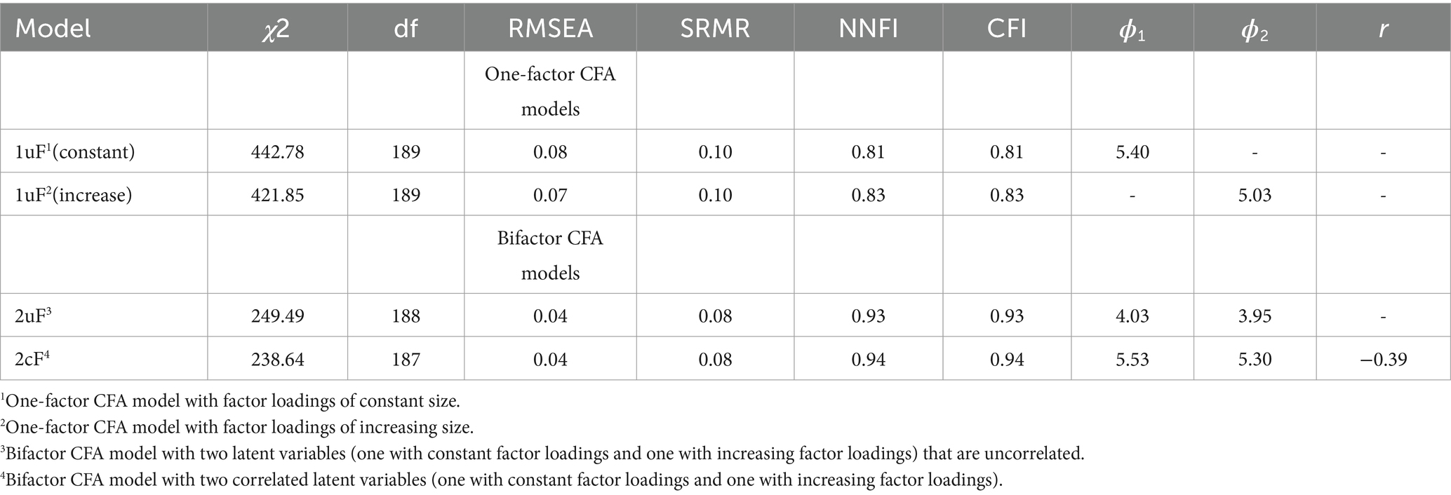
Table 1. Model-fit results, factor variances and factor correlation observed in investigating the relational pattern with the one-factor and bifactor CFA models.
The information on factor variances and the factor correlation is included in the last columns of Table 1 (ϕ1, ϕ2, and r). The standardized covariance representing the factor correlation was negative and of moderate size (see last column). The factor variances for the bifactor models varied between 3.95 and 5.53. For each latent variable there was an increase in size from the model without a correlation to the model with a correlation, as was expected. The increase was 37.2 percent in ϕ1 and 34.2 percent in ϕ2. Furthermore, the factor variances observed for the bifactor CFA model with correlated variables were larger than the corresponding factor variances of the one-factor CFA models. For the first latent variable, ϕ1, the increase was 2.4 percent, and for the second latent variable, ϕ2, it was 5.4 percent. This meant that the factor variances of the one-factor models, which could be expect to account for as much variance as is possible for a single latent variable, were smaller than the corresponding factor variances of the bifactor CFA model. Finally, the mean estimates of variances and the covariance were in line with the assumption that . The estimate of υ was obtained by summing up the variances of 2uF and subtracting this sum form the sum of variances and the covariance of 2cF [(5.53 + (− 0.39) + 5.30) – (4.03 + 3.95) = 2.46 > 0]. In sum, the results supported the hypothesis that a negative factor correlation is associated with overly large factor variance estimates.
The check of the nature of the covariances observed in investigating the 500 covariance matrices revealed that in all cases the covariance was negative so that there was no need for excluding cases. The estimates varied between −0.84 and − 4.17.
Table 2 provides the observed mean factor variances, covariance and factor variance sums. Further, standard deviations are included. The individual factor variance means varied between 3.56 and 5.83 and the factor variance sums between 4.73 and 10.68. As expected, the factor variances observed by the bifactor CFA model with correlated latent variables surmounted the factor variances for the bifactor CFA model without a correlation of latent variables. In the first latent variable there was an increase by 36.2 percent and in the second latent variable 58.4 percent. In the sums of factor variances the increase was 42.5 percent. Additionally, the factor variances were treated as simple observation and compared by t-tests. The outcomes suggested the rejection of the Null hypotheses based on extremely small error probabilities. Furthermore, the mean estimates for variances and the covariance were in line with the assumption that [(4.85 + (− 2.56) + 5.83) – (3.56 + 3.68) = 0.88 > 0].
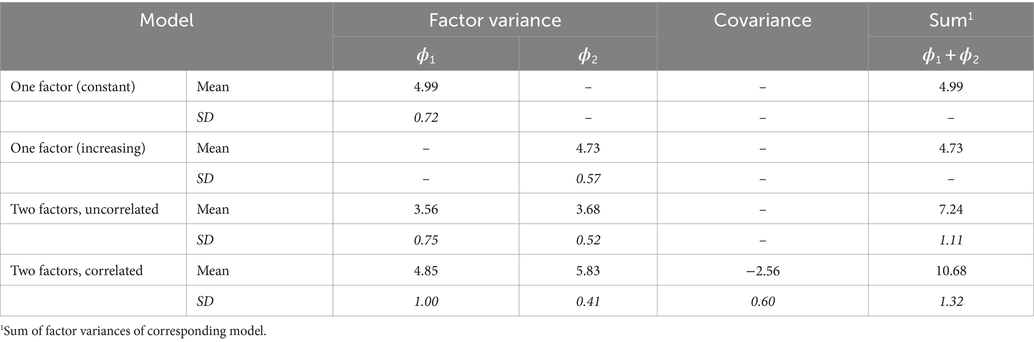
Table 2. Means and standard deviations (in italics) observed in a simulation study by one-factor and two-factor CFA models (N = 500).
Comparing the factor variances observed for the one-factor CFA models with the factor variances observed for the bifactor CFA models revealed that in the first latent variable the estimate by the one-factor CFA model was larger by 2.8 percent and in the second latent variable the estimate of the bifactor CFA model by 23.3 percent. Both factor variance sums for the bifactor CFA models were larger than the factor variances of the one-factor CFA models.
In sum, the main results of the investigation of the relational pattern and the simulation study were in line with the posited statement of an association of a negative factor correlation and an increased size of factor variances.
The account of latent variables for common systematic variation is in the focus of the reported research. In a CFA model with two latent variables that are group latent variables and no correlation among them, each latent variable accounts for its own share of common systematic variation. Allowing them to correlate, it makes a difference whether the correlation is positive or negative. In a positive correlation between the latent variables of a linear measurement model, as is the bifactor model (1), the combination of latent variables accounts for another share of common systematic variation. There are three separate shares of common systematic variation for which two latent variables and their combination account. The model-implied covariance matrix represents these shares in the investigation of data-model fit (3, 4).
In contrast, in negative correlations of latent variables there is a negative component that is expected to account for common systematic variation but cannot be treated as just another share of common systematic variation. The negativity calls the idea of complementary shares of common systematic variation into question. A possible explanation of the effect of negativity could be a compensatory scheme, wherein the negative covariance compensates for overly large accounts of common systematic variation by the two latent variables. Given that modern estimation methods perform according to the expectation–maximization algorithm (28, 29), the description of what happens during iteration cycles could provide an argument in favor of such a compensatory scheme. According to this algorithm, factor loadings and covariance parameters are estimated successively, starting with the estimation of factor loadings. This means that the factor loadings on the latent variables are initially estimated to account for large shares of common systematic variation, followed by the estimation of the covariance parameter. In this way initially achieved overly large factor loadings may subsequently be compensated by a negative covariance estimate. This argument may even hold if factor loadings are fixed instead of being estimated.
The results of investigating the relational pattern and of the simulation study confirm the supposition of negative factor correlations being associated with overly large factor variances. The sizes of factor variances observed together with a negative factor correlation clearly surmount the sizes of factor variances observed under the condition of a factor correlation set to zero. Further, the sums of factor variances displayed the same kind of relationship among each other. Moreover, sums of factor variances characterizing the bifactor CFA model with a correlation of latent variables surmounted the sums of factor variances originating from the two one-factor CFA models whereas the sum of factor variances characterizing the bifactor CFA model without a correlation of latent variables did not.
Factor variances observed together with a negative factor correlation tend to be overly large, as is suggested by the results of the reported investigations. The transfer from observations based on fixed factor loadings to applications making use of free factor loadings suggests that factor loadings observed in combination with negative factor correlations can also be overly large since overly large factor variances must include overly large factor loadings by definition. Since factor loadings provide the basis for factor interpretation (5) and even small differences may count in applications (30), overly large factor loadings should be treated with special care when used in factor interpretation. Further, there are conventional lower limits for factor loadings in item selection for test construction (31). Their application to overly large factor loadings can lead to wrong decisions in the process of constructing a new scale, especially if the factor loadings originate from an application of the bifactor model and the factor correlation happens to be negative. Besides these caveats that may be addressed in future research, the bifactor model can be considered as a useful tool for research that also has frequently been an important part of the authors’ own work.
The bias of factor variances associate with negativity of the factor correlation has so far evaded the attention of research because of various reasons. First, the most popular CFA measurement model that is the original one-factor model (32) employed for the construction and evaluation of scales does not include a factor correlation. Second, there is recency of the topic since the first systematic description and investigation of the CFA bifactor model credited to Reise appeared in 2012 (1) and of estimating unique factor variances in 2019 (17, 33). Third, factor correlations have already been assigned an inconspicuous role in comparing more and less complex models in the framework of the model fit approach (3, 4). Finally, using free factor loadings, variation of loading sizes due to the modification of the model by the inclusion of a factor correlation is unlikely to give reason for concern since variation is considered as” normal” in this context. Therefore, the detection of the bias of factor variances despite these obstacles is an important step in the direction of providing a method for achieving valid estimates of factor variances and factor loadings irrespective of the negativity of the factor correlation.
The predominant use of fixed factor loadings may be considered as a limitation of the reported research since fixed factor loadings do not even play a major role in, for example, text books on confirmatory factor analysis [(e.g., 14)]. Further, using fixed factor loadings does even not mean an advantage regarding model fit since the use of free factor loadings usually leads to the more favorable results regarding model fit. But, free factor loadings are not without problems. As an investigation of the switching-sign problem reveals, the signs of factor loadings estimated in CFA can be incorrect (7). The reason for preferring fixed factor loadings is that they ensure the achievement of clear-cut results. By using fixed factor loadings, the analysis can yield one relevant result for each latent variable, whereas otherwise there would be as many results as there are manifest variables that might not be especially consistent.
A limitation of the presented research is the lack of advice on how to deal with overly large factor variances. The present paper focuses on highlighting the difference between the consequences of positive, negative and zero factor correlations for factor variances of group latent variables and on elucidating the nature of overly large factor variances. Adjustments of overly large factor variances by, for example, relating them to what is observable in one-factor applications or by removing overlapping accounts appear possible but require further study and extensive evaluation. More research is necessary in order to accomplish these tasks.
Overly large factor variances are possible outcomes of CFA on the basis of a bifactor measurement model that includes group latent variables if the correlation between these latent variables happens to be negative. Negative factor correlations signify that estimates of factor variances and corresponding factor loadings may overestimate the shares of common systematic variation for which they account. This should be taken into consideration when using factor loadings for the interpretation and evaluation of the outcomes of investigations using the bifactor model.
The data analyzed in this study is subject to the following licenses/restrictions: data can be requested from the main author. Requests to access these datasets should be directed to KS, ay5zY2h3ZWl6ZXJAcHN5Y2gudW5pLWZyYW5rZnVydC5kZQ==.
KS: Conceptualization, Data curation, Formal analysis, Writing – original draft, Writing – review & editing, Methodology. XR: Conceptualization, Validation, Writing – review & editing. TW: Conceptualization, Validation, Writing – review & editing.
The author(s) declare that financial support was received for the research, authorship, and/or publication of article. This work was supported by the Open-Access-Publikationfonds of Goethe University Frankfurt.
The authors declare that the research was conducted in the absence of any commercial or financial relationships that could be construed as a potential conflict of interest.
The author(s) declared that they were an editorial board member of Frontiers, at the time of submission. This had no impact on the peer review process and the final decision.
All claims expressed in this article are solely those of the authors and do not necessarily represent those of their affiliated organizations, or those of the publisher, the editors and the reviewers. Any product that may be evaluated in this article, or claim that may be made by its manufacturer, is not guaranteed or endorsed by the publisher.
The Supplementary material for this article can be found online at: https://www.frontiersin.org/articles/10.3389/fams.2024.1423726/full#supplementary-material
1. Reise, SP. The rediscovery of Bifactor measurement models. Multivar Behav Res. (2012) 47:667–96. doi: 10.1080/00273171.2012.715555
2. Graham, JM. Congeneric and (essentially) tau-equivalent estimates of score reliability. Educ Psychol Meas. (2006) 66:930–44. doi: 10.1177/0013164406288165
3. Gumedze, FN, and Dunne, TT. Parameter estimation and inference in the linear mixed model. Linear Algebra Appl. (2011) 435:1920–44. doi: 10.1016/j.laa.2011.04.015
4. Jöreskog, KG. A general method for analysis of covariance structure. Biometrika. (1970) 57:239–51. doi: 10.1093/biomet/57.2.239
5. Widaman, KF. On common factor and principal component representations of data: implications for theory and for confirmatory replications. Struct Equ Model. (2018) 25:829–47. doi: 10.1080/10705511.2018.1478730
6. Kline, RB. Principles and practice of structural equation modeling. 2nd ed. New York: The Guilford Press (2005).
7. Tang, D, Boker, SM, and Tong, X. Are the signs of factor loadings arbitrary in confirmatory factor analysis? Struct Equ Model. (2024):1–13. doi: 10.1080/10705511.2024.2351102
8. Rao, OR. Some statistical methods for comparison of growth curves. Biometrics. (1958) 14:1–17. doi: 10.2307/2527726
9. Tucker, LR. Determination of parameters of a functional relationship by factor analysis. Psychometrika. (1958) 23:19–23. doi: 10.1007/BF02288975
10. Schweizer, K, Ren, X, Wang, T, and Zeller, F. Does the constraint of factor loadings impair model fit and accuracy in parameter estimation? Int J Stat Prob. (2015) 4:40–50. doi: 10.5539/ijsp.v4n4p40
11. McArdle, JJ. Latent variable modeling of differences and change with longitudinal data. Annu Rev Psychol. (2009) 60:577–605. doi: 10.1146/annurev.psych.60.110707.163612
12. Troche, SJ, Schweizer, K, and Rammsayer, TH. The relationship between attentional blink and psychometric intelligence: a fixed-links model approach. Psychol Sci Q. (2009) 51:432–48.
13. Wang, T, Ren, X, Li, X, and Schweizer, K. The modeling of temporary storage and its effect on fluid intelligence: evidence from both Brown-Peterson and Complex span tasks. Intelligence. (2015) 49:84–93. doi: 10.1016/j.intell.2015.01.002
14. Brown, TA. Confirmatory factor analysis for applied research. 2nd ed. New York: The Guilford Press (2015).
15. Gonzalez, R, and Griffin, D. Testing parameters in structural equation modeling: every “one” matters. Psychol Methods. (2001) 6:258–69. doi: 10.1037/1082-989X.6.3.258
16. Steiger, JH. When constraints interact: a caution about reference variables, identication constraints, and scale dependencies in structural equation modeling. Psychol Methods. (2002) 7:210–27. doi: 10.1037/1082-989X.7.2.210
17. Schweizer, K. Scaling variances of latent variables by standardizing loadings: applications to working memory and the position effect. Multivar Behav Res. (2011) 46:938–55. doi: 10.1080/00273171.2011.625312
18. Klopp, E, and Klößner, S. The impact of scaling methods on the properties and interpretation of parameter estimates in structural equation models with latent variables. Struct Equ Model. (2020) 28:182–206. doi: 10.31219/osf.io/c9ke8
19. Little, TD, Slegers, DW, and Card, NA. A non-arbitrary method of identifying and scaling latent variables in SEM and MACS models. Struct Equ Model. (2006) 13:59–72. doi: 10.1207/s15328007sem1301_3
20. Schweizer, K, Troche, S, and DiStefano, C. Scaling the variance of a latent variable while assuring Constancy of the model. Front Psychol. (2019) 10:887. doi: 10.3389/fpsyg.2019.00887
21. Jöreskog, KG. A general approach to confirmatory maximum likelihood factor analysis. Psychometrika. (1969) 34:183–202. doi: 10.1007/BF02289343
22. Ren, X, Wang, T, Sun, S, Deng, M, and Schweizer, K. Speeded testing in the assessment of intelligence gives rise to a speed factor. Intelligence. (2017) 66:64–71. doi: 10.1016/j.intell.2017.11004
23. Borter, N, Schlegel, K, and Troche, S. How Speededness of a reasoning test and the complexity of mental speed tasks influence the relation between mental speed and reasoning ability. J Intelligence. (2023) 11:89. doi: 10.3390/jintelligence11050089
24. Schweizer, K, Wang, T, and Ren, X. On the detection of Speededness in data despite selective responding using factor analysis. J Exp Educ. (2020) 90:486–504. doi: 10.1080/00220973.2020.1808942
25. Jöreskog, KG, and Sörbom, D. Interactive LISREL: user’s guide. Lincolnwood, IL: Scientific Software International Inc (2001).
26. Jöreskog, KG, and Sörbom, D. LISREL 8.80. Lincolnwood, IL: Scientific Software International Inc (2006).
27. DiStefano, C. Examining fit with structural equation models In: K Schweizer and C Distefano, editors. Principles and methods of test construction. Göttingen: Hogrefe Publishing (2016). 166–93.
28. Rubin, DB, and Thayer, DT. EM algorithms for ML factor analysis. Psychometrika. (1982) 47:69–76. doi: 10.1007/BF02293851
29. McLachlan, GJ. Computation: expectation-maximization algorithm In: International encyclopedia of the social and behavioral sciences. 2nd ed. Amsterdam: Elsevier (2016).
30. Geminiani, E, Ceulemans, E, and Rouver, K. Testing for factor loading differences in mixture simultaneous factor analysis: a Monte Carlo simulation-based perspective. Struct Equ Model. (2020) 28:391–409. doi: 10.1080/10705511.2020.1807351
31. Bandalos, DL, and Gerstner, JJ. Using factor analysis in test construction In: K Schweizer and C Distefano, editors. Principles and methods of test construction. Göttingen: Hogrefe Publishing (2016). 26–51.
32. Jöreskog, KG. Statistical analysis of sets of congeneric tests. Psychometrika. (1971) 36:109–33. doi: 10.1007/BF02291393
Keywords: factor variance, factor loading, confirmatory factor analysis, bifactor model, group latent variable, group factor
Citation: Schweizer K, Ren X and Wang T (2024) Negativity of factor correlations biases the sizes of factor variances in bifactor CFA models. Front. Appl. Math. Stat. 10:1423726. doi: 10.3389/fams.2024.1423726
Edited by:
Min Wang, University of Texas at San Antonio, United StatesReviewed by:
Shen Zhang, Sanofi U.S., United StatesCopyright © 2024 Schweizer, Ren and Wang. This is an open-access article distributed under the terms of the Creative Commons Attribution License (CC BY). The use, distribution or reproduction in other forums is permitted, provided the original author(s) and the copyright owner(s) are credited and that the original publication in this journal is cited, in accordance with accepted academic practice. No use, distribution or reproduction is permitted which does not comply with these terms.
*Correspondence: Karl Schweizer, ay5zY2h3ZWl6ZXJAcHN5Y2gudW5pLWZyYW5rZnVydC5kZQ==
†ORCID: Karl Schweizer, https://orcid.org/0000-0002-3143-2100
Disclaimer: All claims expressed in this article are solely those of the authors and do not necessarily represent those of their affiliated organizations, or those of the publisher, the editors and the reviewers. Any product that may be evaluated in this article or claim that may be made by its manufacturer is not guaranteed or endorsed by the publisher.
Research integrity at Frontiers
Learn more about the work of our research integrity team to safeguard the quality of each article we publish.