Predicting successful trading in the West Texas Intermediate crude oil cash market with machine learning nature-inspired swarm-based approaches

The subject of predicting global crude oil prices is well recognized in academic circles. The notion of hybrid modeling suggests that the integration of several methodologies has the potential to optimize advantages while reducing limitations. Consequently, hybrid techniques are extensively used in contemporary research. In this paper, a novel decompose-ensemble prediction approach is proposed by integrating various optimization algorithms, namely biography-based optimization (BBO), backtracking search algorithm (BSA), teaching-learning-based algorithm (TLBO), cuckoo optimization algorithm (COA), multi-verse optimization (MVO), and multilayer perceptron (MLP). Furthermore, the aforementioned approaches, namely BBO-MLP, BSA-MLP, and TLBO-MLP, include the de-compose-ensemble technique into the individual artificial intelligence model in order to enhance the accuracy of predictions. In order to validate the findings, the forecast is conducted using the authoritative data on oil prices. This study will use three primary indicators, including EMA 20, EMA 60, EMA 100, ROC, and AUC assessments, to assess and evaluate the efficacy of the five methodologies under investigation. The below findings are derived from the conducted research: Based on the achieved AUC values of 0.9567 and 0.9429, it can be concluded that using a multi-verse optimization technique is considered the most suitable strategy for effectively handling the dataset pertaining to crude oil revenue. The next four approaches likewise have a significant AUC value, surpassing 0.8. The AUC values for the BBO-MLP, BSA-MLP, TLBO-MLP, and COA-MLP approaches were obtained as follows: (0.874 and 0.792) for training and testing stages, (0.809 and 0.792) for training and testing stages, (0.9353 and 0.9237) for training and testing stages, and (0.9092 and 0.8927) for training and testing stages, respectively. This model has the potential to contribute to the resolution of default probability and is very valuable to the credit card industry. Broadly speaking, this novel forecasting approach serves as a notable predictor of crude oil prices.

1 Introduction

Crude oil plays a crucial role in sustaining the global economy. The economic development and prosperity of both industrialized and emerging countries depend on its materiality. Furthermore, it is noteworthy that political events, dramatic weather phenomena and financial market speculation have a significant influence on the crude oil market and thus contribute to the volatility of oil market prices (1, 2). Oil price fluctuations have a significant impact on a wide range of products and services and have direct economic and social consequences. Therefore, predicting price direction is of significant importance to minimize the negative impact of price volatility. Unfortunately, important information such as oil supply, demand stocks and GDP are not included in the daily data, making prediction more difficult (3, 4).

Crude oil has significant value as a globally sought-after raw material and serves as a basic resource for several industries. Crude oil plays an essential role in the economy of all nations. As a result, oil prices have become a growing concern for governments, companies and investors. The price of oil can be directly influenced by a variety of domestic and foreign market factors such as speculation, economic slowdowns and geopolitical events. These special properties contribute to the fact that the oil market tends to experience regular price fluctuations. In July 2008, the market price for each barrel of West Texas Intermediate (WTI) crude oil exceeded $145. However, as a result of the financial crisis, there was a significant decline in oil prices of over 80 percent, which ultimately reached a low of around US$33 per barrel at the end of 2008. A limited number of academic articles (5–7) have conducted an examination of market microstructure to gain a deeper understanding of the complex dynamics in crude oil markets.

Since the outbreak of the 1973–1974 oil crisis, there has been a significant influx of academic research into forecasting crude oil prices. This section provides a brief overview of relevant and current scientific research. Moshiri and Foroutan (8) conducted an analysis of disorder and nonlinearity in crude oil futures prices. Various statistical and economic studies indicate that the time series of futures prices exhibits characteristics of stochasticity and nonlinearity. In addition, the authors conducted a comparison of artificial neural networks (ANN) and linear and nonlinear models, including autoregressive moving average (ARMA) and generalized autoregressive conditional heteroscedasticity (GARCH), to predict future crude oil futures prices. The researchers found that ANNs have a significant impact and provide statistically significant predictions. Two important observations can be made about this study. The authors began the process by providing raw data to the ANN. In addition, the neural network was trained with data that is no longer current, namely from the years 1983 to 2000. In this paper, we will next provide arguments that refute the validity of the two theses mentioned above.

Wang et al. (9) in their study, provide a hybrid approach aimed at predicting monthly fluctuations in crude oil prices. The model has three distinct components. The researchers develop a rule-based system, ANN and autoregressive integrated moving average (ARIMA) models, as well as a hybrid approach using web mining techniques. The three components operate autonomously prior to converging to provide the resultant product. It was shown that the integration of all three models using a non-linear approach yielded superior performance compared to the individual performance of each model. Nevertheless, this approach has some limitations. The text mining model 3 utilizes a rule-based system that relies on a knowledge base provided by humans. The problematic and untrustworthy nature of this method arises from the divergent perspectives of experts on the subject matter.

Furthermore, both the information base and the rules have not been made accessible to the general public. Predicting successful trading in the West Texas Intermediate crude oil cash market using machine learning nature-inspired swarm-based approaches is a crucial aspect of economic development and sustainability (10). Various studies have explored the application of different algorithms to enhance prediction accuracy, such as the hybridization of artificial immune system and ant colony optimization for function approximation (11), as well as utilizing artificial neural networks with the whale optimization algorithm to improve forecasting accuracy by up to 22% compared to basic models (12). Jovanović et al. (10) proposes a modified version of the salp swarm algorithm to improve the accuracy of crude oil price prediction. The approach is validated on real-world West Texas Intermediate (WTI) crude oil price data and outperforms other metaheuristics. Chen (11) show HIAO algorithm improves accuracy for crude oil spot price prediction. Sohrabi et al. (3) predicts WTI oil prices using ANN-WOA algorithm. In another study, Das et al. (13) focuses on forecasting crude oil prices using hybrid approach. They find out hybrid model using ELM and IGWO for crude oil forecasting, predicts crude oil prices efficiently for short-term. Additionally, employing extreme learning machines with the improved grey wolf optimizer has shown promising results in forecasting crude oil rates, outperforming other models like ELM-PSO and ELM-GWO in terms of convergence rate and mean square error (4). These advancements in machine learning models, such as ANN-PSO, have proven effective in accurately predicting long-term crude oil prices, aiding investors in making informed decisions and potentially increasing long-term profits (14). Xie et al. (15) developed a support vector machine (SVM) model to analyze and predict monthly fluctuations in crude oil prices. According to the authors, the SVM outperforms the multilayer perceptron (MLP) and autoregressive integrated moving average (ARIMA) models in terms of out-of-sample predictions. However, both studies used monthly pricing data, resulting in a significant reduction in the sample size. Furthermore, it should be noted that the sample includes data collected in 1970, which might be considered quite outdated. The use of commodity futures prices for the estimation of spot prices is based on the underlying assumption that futures prices exhibit a higher degree of responsiveness to fresh market information compared to spot prices. Silvapulle and Moosa (16) believe that futures trading offers a multitude of advantages, including reduced transaction costs, enhanced liquidity, and diminished initial capital prerequisites. This phenomenon enhances the attractiveness for investors to react to new information rather than taking an immediate position in the spot market. This theory is applicable to a wide range of commodities traded on financial markets, with a specific relevance to the energy sector (17, 18). When new information emerges about the oil market, investors have the option to adopt a position (either buying or selling) in either the spot or futures market. Opting for immediate engagement in the spot market may not always be the most advantageous course of action in light of many factors such as substantial transaction charges, storage fees, and shipping expenses. This is particularly true when investors exhibit no inclination towards the specific commodity, but rather engage in hedging against an alternative commodity or speculating on arbitrage prospects via their investments in the market. Based on the aforementioned reasons (16), the futures market presents a far more attractive option for investors to respond to emerging information in this particular scenario. Brooks et al. (19) used 10 min high-frequency data of the FTSE index to examine the lead-lag connection. Based on the authors’ findings, it is suggested that the lead-lag4 connection has a maximum duration of 30 min. The outcomes of the study indicate that it is possible to use future price fluctuations as a means to predict alterations in spot pricing. Bopp and Sitzer (20) examined the extent to which futures prices effectively predicted upcoming spot prices in the heating oil market. This study aims to determine to what extent the inclusion of forward prices in econometric models could improve their predictive capabilities. Based on the available data, it can be seen that futures contracts with a maturity of 1 or 2 months have statistical significance in predicting spot prices. In other words, it is necessary for novel data to be available. Chan (21), a research was conducted to examine the relationship between lags and leads in the context of the S&P 500. The results of this study produced results consistent with previous research. The researcher made the observation that the futures market serves as the primary channel for disseminating market-wide information.

Conversely, the cash market serves as the principal repository of information pertaining to a particular corporation. Additionally, Silvapulle and Moosa (16) indicates that the lead-lag relationship in the oil market is not consistently present and exhibits temporal variations. Coppola (22) conducted a study on the crude oil market, revealing findings that suggest futures contracts might potentially serve as indicators of future spot price trends. Abosedra and Baghestani (23) examined the monthly future prices as a means of doing long-term forecasting. Accurate projections were provided to policymakers only by futures contracts with durations ranging from one to 12 months in the future.

This research presents five ANN models that are used for the purpose of predicting the trade of crude oil based on the West Texas Intermediate price. The subsequent sections of this article are organized in the following manner: section 2 provides an analysis of database collecting, while section 3 delves into the topics of preprocessing and technique. Section 4 of the paper delves into the examination and analysis of the research outcomes, while section 5 serves as a conclusion that encapsulates the whole of the study.

2 Database collection

The determination of data frequency and size has significant importance in the realm of network architecture. The determination of the intended consequence largely governs this matter. Short-term projections often rely on high-frequency data, such as intraday or daily data, for analysis and forecasting purposes. Nevertheless, accessing and obtaining this data may sometimes be challenging and come with exorbitant expenses. Weekly and monthly data are preferred for predicting periods due to their lower levels of noise. The durability of the data is a crucial factor to take into account. The accuracy of the neural network’s generalization improves as the number of data points increases in the context of ANN. Nevertheless, this assertion does not consistently hold true in the context of economic or financial time series. Due to the dynamic nature of economic situations, the use of obsolete information may have a detrimental impact on outcome predictions. This is because including irrelevant information into the training process might lead to a suboptimal generalization of the model (24, 25). This study uses the following set of five-time series data. The abbreviation “WTI” refers to West Texas Intermediate. Once the data has been partitioned into training and testing sets, the training set comprises 80% of the data while the remaining 20% is allocated for testing purposes, which is conducted outside the sample period, often spanning one financial year (Figure 1).

Figure 1

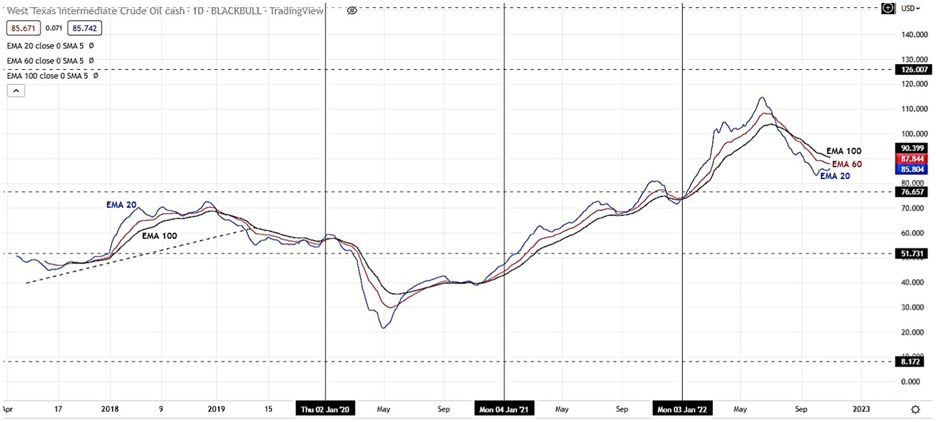
Figure 1. The process of real time data collection.

The selection of the three indications in Figure 2 was justified. The prices of West Texas Intermediate (WTI) are subject to substantial impact from three price basis indicators, often referred to as exponential moving averages (EMAs). The exponential moving average (EMA) functions similarly to the simple moving average (SMA) by monitoring the trajectory of the trend as time progresses. The exponential moving average (EMA) exhibits a preference for including more recent data as compared to the simple moving average (SMA), which relies on a straightforward calculation of the average price. A technical chart is a tool used in financial analysis to assess the fluctuations in the value of a financial instrument within a certain period. The exponential moving average (EMA) is a variant of the weighted moving average (WMA) that places more emphasis on more recent price data (Figures 2–4); (Table 1).

Figure 2

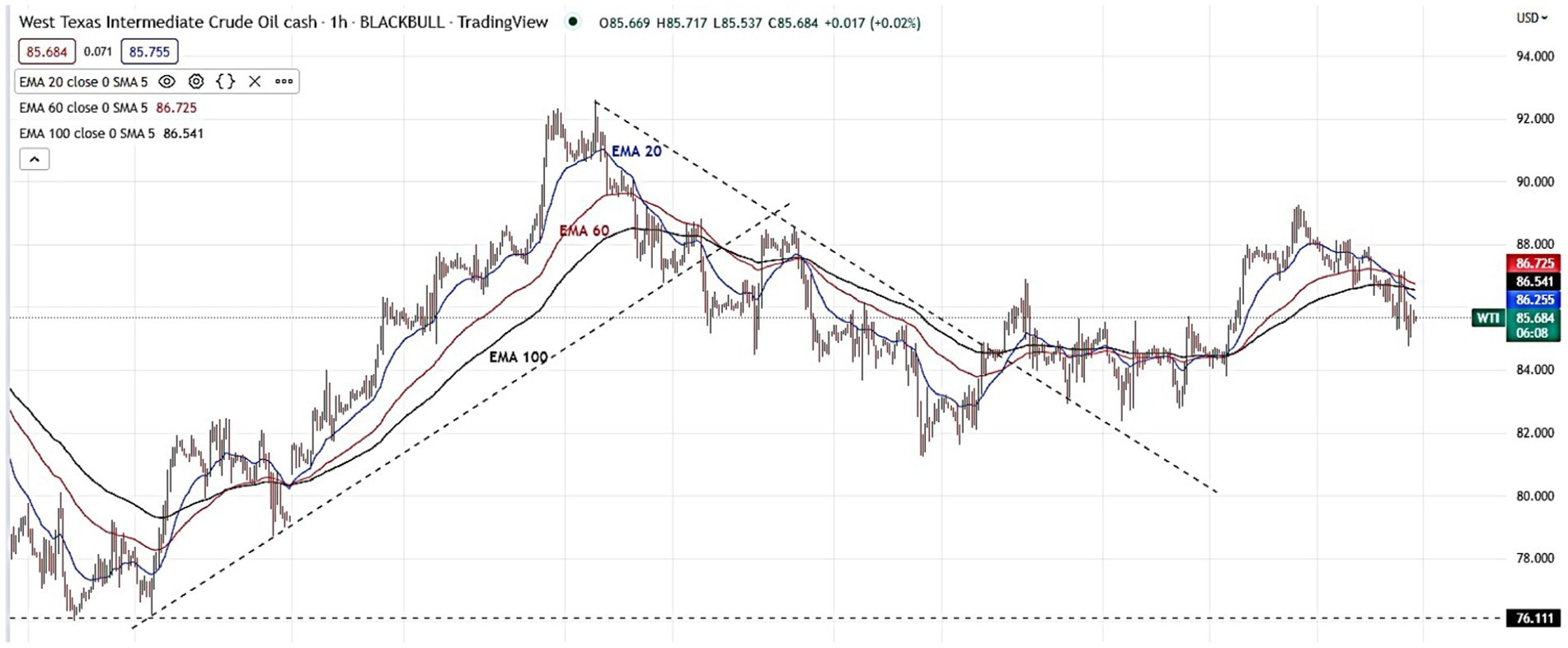
Figure 2. The example of EMA 20, 60 and 100 in 30 min timeframe.

Figure 3

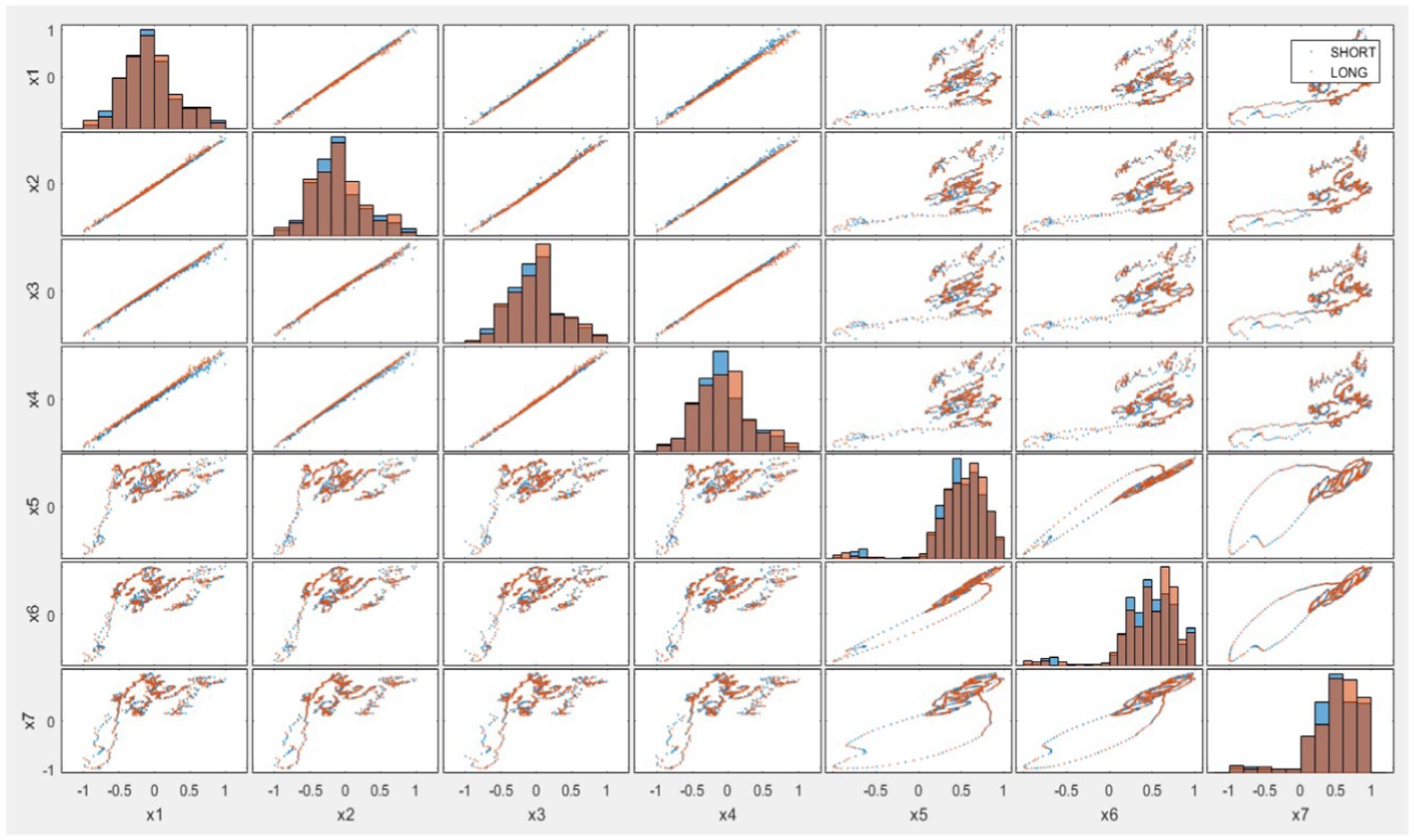
Figure 3. Description of input layers (x1–x7) versus output.

Figure 4

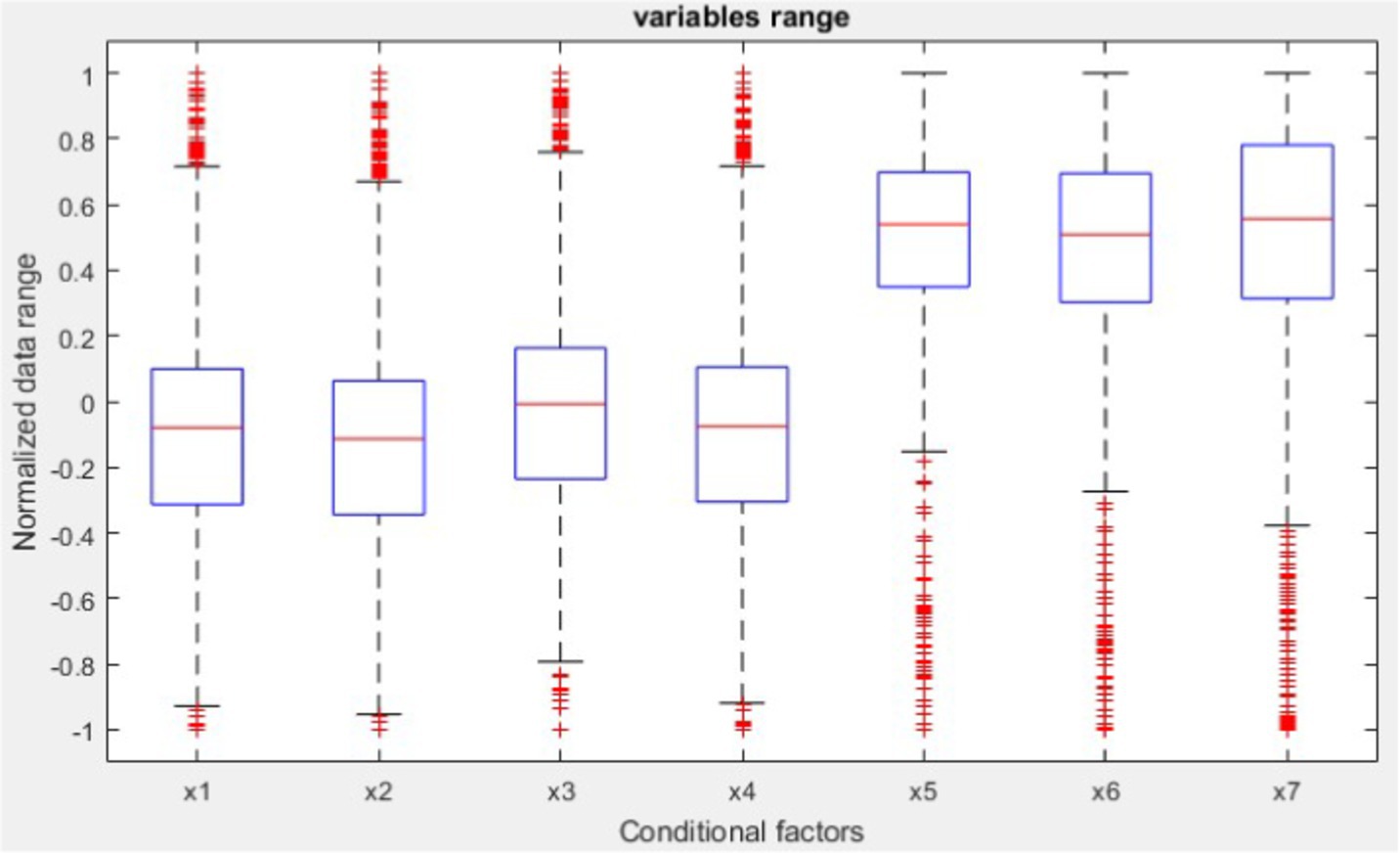
Figure 4. Conditional factors.

Table 1

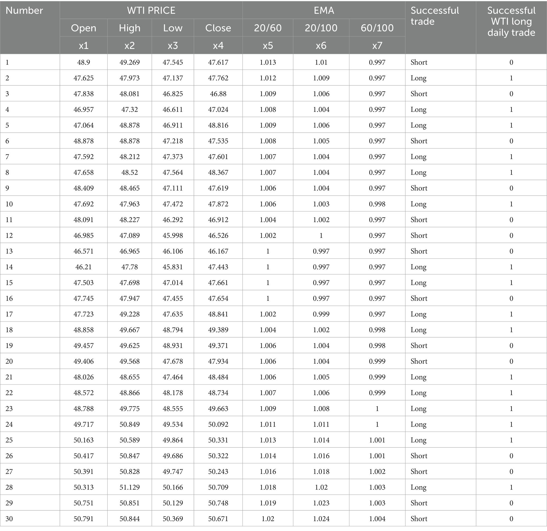
Table 1. example of input dataset and WTI price detail in daily time frame.

3 Methodology

Market participants will react to this information in accordance with their expertise, positions, forecasts, evaluations, and other relevant factors, assuming the market is seen as a system that incorporates past and current information as inputs. The output or closing price is determined by the collective efforts of market participants. In order to replicate the behavior of the market, a model must choose use a subset of the accessible information, endeavor to align it with the desired objective, and then provide a forecast with a certain level of accuracy, often referred to as an error (26). Figure 5 depicts the study flowchart, which encompasses the input components used for the purpose of predicting the result (Figure 5).

Figure 5

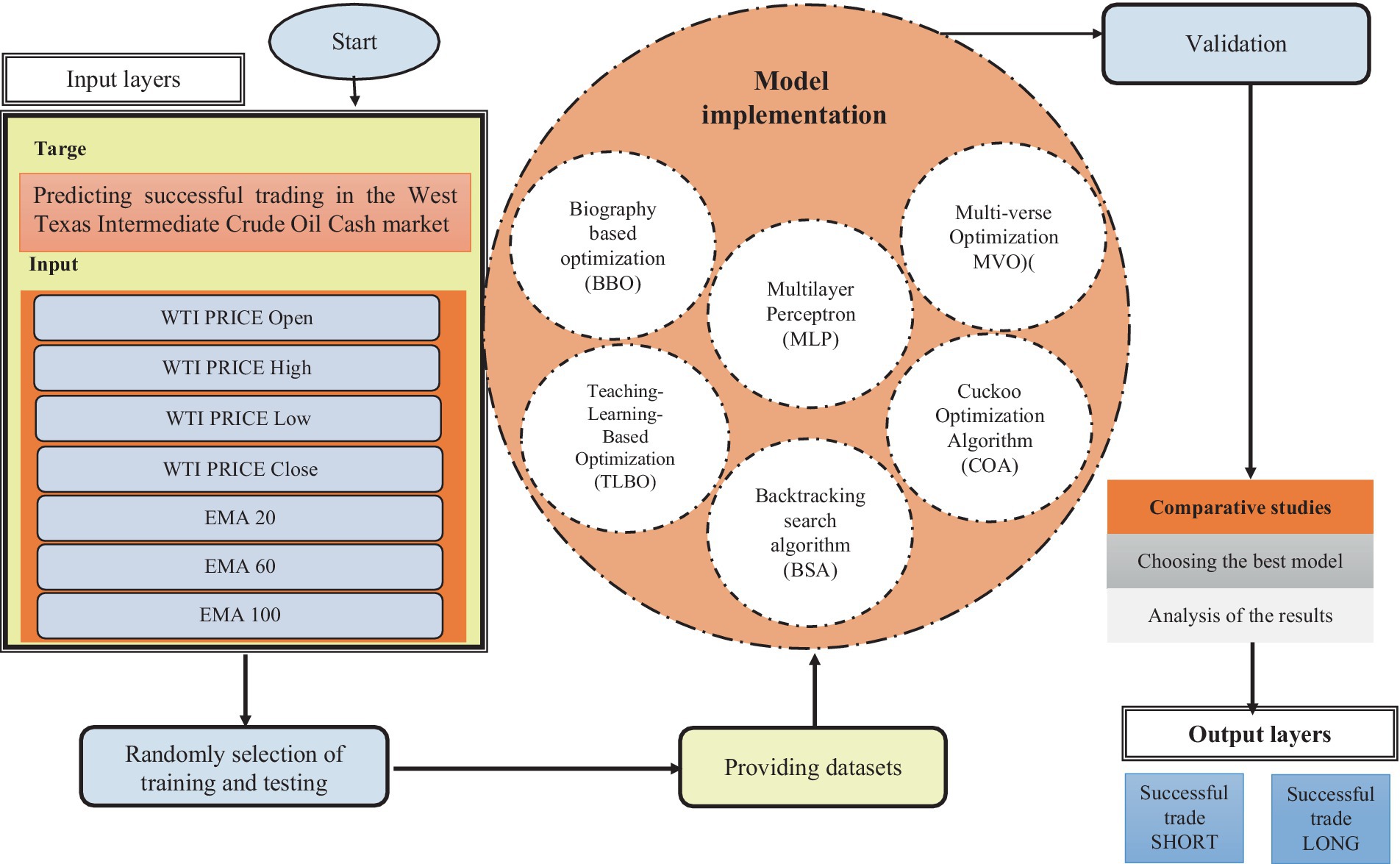
Figure 5. Research flowchart.

3.1 Artificial neural network

There are three primary prerequisites for every good ANN model in the widest sense (26):

• In-sample precision.

• The model’s capacity to function with new data.

• Stability and uniformity of network output.

ANNs replicate the cognitive learning mechanism of the human brain. The brain obtains information via processes such as learning, remembering, and generalization (27). Computer software is responsible for executing essential activities, which include generating fresh data based on preexisting data. Artificial neurons are organized into artificial neural networks, as shown by previous studies (28, 29). The clustering process is executed in sequential stages, which are afterwards interconnected. All neural networks possess a fundamentally similar structure. Certain neurons within this configuration are externally affixed to facilitate the reception of inputs, whilst others are externally linked to facilitate the transmission of outputs. The neurons that survive are situated inside the buried layers. Several factors need to be taken into account in order to assure the achievement of the aforementioned objectives. The testing process encompasses several aspects, such as data preparation procedures, the number of layers used, the selection of activation functions, the determination of the learning rate, the duration of the training process, the utilization of first- and second-order optimization approaches, and the determination of the number of hidden neurons. The determination of the experimental design for all preliminary trials was based on a systematic exploration of various trial combinations. The determination of the optimal number of hidden neurons is a critical aspect in the use of neural networks, as an excessive quantity may lead to overfitting, while an insufficient quantity may result in under fitting. The objective is to use the minimum number of neurons that may provide the most significant results beyond the given sample (24). There is a lack of established protocols for addressing this issue. Typically, heuristics algorithms and evolutionary computing methodologies are used. Each of these tactics has both advantages and disadvantages associated with it. The implementation of a technique including a limited number of neurons, together with the training and evaluation of networks for a certain number of iterations, has been identified as a necessary approach in reference (25). The number of concealed neurons was increased until the desired amount was achieved (30). Furthermore, the researchers in reference (31) used this methodology to develop a lucrative ANN trading system specifically designed for the Australian stock market. In the study conducted by the authors (32), it was observed that a single neuron was disguised for every new input or delayed value of the same variable. This process continued until a total of 10 neurons were hidden.

Furthermore, the stability of each neuronal count was assessed by examining each network twice using different weight values (33). The performance of each model was correctly judged by averaging the outcomes of the three trials. The network configuration of this experiment is shown in Figure 6.

Figure 6

Figure 6. ANN architecture for predicting successful trading.

The number of hidden layers in an ANN can vary depending on the complexity of the problem. Common configurations include 2 hidden layers, often determined through experimentation or optimization. The number of neurons in each layer is also variable and can range from a few dozens to several hundred or more, depending on the specific requirements of the model and the complexity of the task. All these hyperparameters, including the number of hidden layers, the number of neurons in each layer, learning rate, batch size, and others, can be considered as unknowns and determined/optimized using metaheuristic algorithms. Metaheuristic algorithms such as biography-based optimization (BBO), backtracking search algorithm (BSA), teaching-learning-based optimization (TLBO), cuckoo optimization algorithm (COA), and multi-verse optimization algorithm (MVO) can be employed to search the hyperparameter space efficiently, finding the best set of parameters that optimize the performance of the ANN. In designing and optimizing ANNs, several hyperparameters need to be carefully chosen and potentially optimized. These include:

Hyperparameters:

- Learning rate: The rate at which the model updates its weights during training.

- Batch size: The number of training examples used in one iteration of training.

- Number of epochs: The number of times the entire training dataset is passed through the network.

- Momentum: A factor that helps accelerate the gradient descent algorithm by considering the past gradients.

- Weight initialization: The method used to initialize the weights of the network (e.g., Xavier, He initialization).

- Regularization parameters: Such as L1/L2 regularization coefficients to prevent overfitting.

- Dropout rate: The fraction of neurons to drop during training to prevent overfitting.

- Activation function parameters: Any specific parameters required for certain activation functions.

Transfer functions (activation functions):

- Sigmoid: Used primarily in the output layer for binary classification problems.

- Tanh: Often used in hidden layers, it outputs values between −1 and 1.

- ReLU (Rectified Linear Unit): A popular choice for hidden layers due to its ability to mitigate the vanishing gradient problem.

- Leaky ReLU: An improved version of ReLU that allows a small, non-zero gradient when the unit is not active.

- Softmax: Used in the output layer for multi-class classification problems.

3.2 Hybrid model development

This study assesses and compares the effectiveness of five innovative neural computing optimizations (BBO-MLP, BSA-MLP, TLBO-MLP, COAMLP, and MVO-MLP) when used to the task of predicting crude oil cash flow. The integration of optimization algorithms from various categorization approaches within ANNs enhances their ability to accurately predict and analyze complex data patterns. This process involves incorporating BBO, BSA, TLBO, COA, and MVO into the training and optimization phases of ANNs. BBO is inspired by the migration patterns of species. In the context of ANNs, BBO can be used to optimize the weights and biases of the network by simulating the sharing of information among a population of solutions. This helps in escaping local optima and finding a more globally optimal solution for the network parameters. BSA employs a systematic search methodology that backtracks to previous solutions to explore the solution space efficiently. When integrated with ANNs, BSA enhances the training process by systematically exploring and exploiting the weight space, leading to improved convergence rates and accuracy. TLBO mimics the teaching-learning process in a classroom. In ANNs, the TLBO algorithm can be used to iteratively refine the network parameters. The “teacher” phase improves the mean solution by guiding the population towards better solutions, while the “learner” phase allows solutions to interact and learn from each other, enhancing the network’s learning capability. COA is inspired by the brood parasitism behavior of some cuckoo species. It uses a combination of local and global search mechanisms to find optimal solutions. When applied to ANNs, COA helps in optimizing the network parameters by balancing exploration and exploitation, which leads to better generalization and performance of the network. MVO is based on the concepts of physics, particularly the interaction of universes through wormholes. In ANNs, MVO can be utilized to optimize the network by allowing multiple candidate solutions to interact and converge towards the best solution. This algorithm enhances the diversity of solutions and avoids premature convergence, leading to more robust and accurate models. Each of these optimization algorithms can be integrated into the ANN training process to fine-tune the network parameters. This integration involves embedding the optimization routines into the backpropagation algorithm or using them as standalone optimizers to adjust weights and biases iteratively. Once the required hybrids have been constructed, their capability for learning and generalization is evaluated by analyzing data obtained from both the training and testing phases. This research utilizes two precision measures, namely the mean average error (MAE) correlation metric and the root mean square error (RMSE) error measurements. The formulation of these indices is as follows Eqs. 1, 2:

$\begin{array}{ll}\mathrm{RMSE}={\left[N^{-1}{\displaystyle \sum }_{i=1}^N{\left(y_{\mathrm{measured},i}-y_{\mathrm{predicted},i}\right)}^2\right]}^{0.5}& (1)\end{array}$

$\begin{array}{ll}\mathrm{MAE}=\frac{1}{N}{\displaystyle \sum }_{i=1}^N\left(y_{\mathrm{measured},i}-y_{\mathrm{predicted},i}\right)& (2)\end{array}$

where n deotes the observations number. $y_{\mathrm{measured},i}$ represents the determined value of the ith data number, $y_{\mathrm{predicted},i}$ represents the anticipated value of the ith data number. RMSE should be equal to 0, in the most optimal model.

3.2.1 Biography-based optimization

Similar to conventional problem-solving methodologies, biogeography may be seen as nature’s mechanism for the dispersal of species. Let us consider a hypothetical scenario where a problem is presented along with a set of possible remedies. The problem may manifest itself in several domains of human existence, as long as we are able to measure the effectiveness of a suggested solution. The field of biogeography, which examines the geographical and temporal distribution of biological species, has had a significant impact on the development of biogeography-based optimization (BBO) throughout time. A habitat H (𝐻 ∈ SIV^𝑛) is a multidimensional array of n variables that represents a possible gas chimney alternative.

The suitability index variable (SIV) is a quantitative representation of all favorable characteristics found within a given ecosystem. The habitat suitability index (HSI) is a metric used to assess the fitness of a given environment by quantifying its quality. The habitat that has the highest HIS is considered to be the most optimal initial feature subset. The habitat vector utilizes migration and mutation mechanisms to determine the optimal solution. The immigration rate (k) is proportional to the probability that SIVs will move into habitat H, which is proportional to λ, and the probability that the source of modification originates from habitat 𝐻_𝑗 is proportional to 𝜇_𝑖.

The number of species in a habitat determines immigration and emigration rates. Each generation is computed using Eqs. 3, 4.

$\begin{array}{ll}{\lambda }_i=I\times \frac{\left[1-R\left(i\right)\right]}{S_{\max }}& (3)\end{array}$

$\begin{array}{ll}{\mu }_i=E\times \frac{\left[1-R\left(i\right)\right]}{S_{\max }}& (4)\end{array}$

The rank of the ith individual, denoted as R(i), is determined. $S_{\max }$ represents the largest species count, whereas I represent the maximum immigration rate and E represents the maximum emigration rate. The mutation operator is a stochastic mechanism that introduces random adjustments to the habitat’s SIVs, influenced by the habitat’s a priori probability of existence. The utilization of the mutation technique facilitates the enhancement of solutions characterized by a low HSI, while solutions exhibiting a high HSI have the potential to experience even greater improvement. The selected feature of the ith solution is substituted with a value that is randomly produced, in accordance with the mutation rate that has been provided in Eq. 5:

$\begin{array}{ll}{m}_i=m_{\max }\left[1-\frac{R\left(i\right)}{P_{\max }}\right]& (5)\end{array}$

where 𝑚_𝑖 denotes the mutation rate of the ith individual, $m_{\max }$ is the maximum mutation rate, 𝑝_𝑖 is the probability of the ith individual given by Eq. 6:

$\begin{array}{ll}{p}_j=p_j\left[1-{\lambda }_j-{\mu }_j\right]+p_{j-1}{\lambda }_{j-1}+p_{j+1}{\mu }_{j+1}& (6)\end{array}$

where $p_{\max }$ denotes the maximum probability calculated among all probabilities. The algorithm maintains elitism to keep the population’s best solutions. This prevents immigration from diminishing the quality of the most effective solutions. Figure 2 depicts the entire BBO method for determining the optimal subsets of features for interpreting gas chimneys and hydrocarbons. As with other evolutionary algorithms, BBO’s superior solutions have a greater propensity to share their data, resulting in the best characteristics.

Unique among evolutionary algorithms, BBO’s migration process permits the modification of earlier solutions (34). BBO and GA increase population diversity via mutation.

BBO successfully identifies important chimney disturbances and correlations between seismic features by identifying the pertinent non-redundant seismic feature for straightforward and effective interpretation (35).

3.2.2 Backtracking search algorithm

The BSA method is a revolutionary approach designed for solving numerical optimization problems that include variables, including values that are real-valued (36). In contrast to previous evolutionary algorithms, the BSA method addresses many issues, including vulnerability to control variables, premature convergence, and slow computing (37). Therefore, the BSA has just one parameter. Additionally, the performance of BSA is not too reliant on the initial value of this parameter. The BSA population is generated by the use of genetic operators, namely selection, mutation, and crossover. The term refers to the algorithmic approach used in the field of computer science for the purpose of locating a certain value or achieving a desired objective. The presence of a specific objective is crucial in this context, and the optimal strategy must be selected from the range of alternatives that are now accessible.

Furthermore, the use of the search-direction matrix and the implementation of the search-space boundary amplitude control enhance the system’s ability to explore and utilize its surroundings. The BSA has the capability to enhance the search direction by using a memory component that stores a population with random characteristics. The initial value of this parameter does not have an impact on the problem-solving efficacy of BSA. The BSA has a fundamental framework that exhibits effectiveness, expediency, and proficiency in addressing multimodal challenges, hence facilitating its ability to swiftly accommodate diverse numerical optimization problems. The BSA population formation experimental approach has been enhanced with the inclusion of two more crossover and mutation operators. The technique used by BSA in generating trial populations and managing the amplitude of the search-direction matrix and search-space boundaries is very successful in facilitating both exploration and exploitation.

3.2.2.1 Population initialization

The population is the total number of individuals uniformly distributed across the search area. It may also be stated as Eq. 7:

$\begin{array}{ll}{P}_{i,j}~U\left({\mathrm{low}}_j{\mathrm{,up}}_j\right)& (7)\end{array}$

where i and j represent the population size and issue dimension, low and up represent each individual’s minimum and maximum values, and U represents the uniform distribution in each person.

3.2.2.2 Selection-I

The BSA selection focuses on direction-improving memory data in the first stage. OldP’s historical population is what we are referring to here as the memory. The initial population of people is determined at random as follows Eq. 8:

$\begin{array}{ll}\mathrm{old}{P}_{i,j}~U\left({\mathrm{low}}_j{\mathrm{,up}}_j\right)& (8)\end{array}$

At the start of each iteration of BSA, the oldP is redefined using the “if-then” expression (38).

$\begin{array}{ll}\mathrm{if}a<b\mathrm{then}\mathrm{old}P:=P|a,b~\left(0\mathrm{,}1\right)& (9)\end{array}$

The update operation, denoted by the symbol “≔,” is defined so that Eq. 9 guarantees that BSA labels a population as belonging to the historical population and retains this designation until it undergoes a change. Subsequently, the arrangement of persons in oldP undergoes a random permutation through the utilization of a shuffling function, as described in Eq. 10:

$\begin{array}{ll}\mathrm{old}P:=\mathrm{permuting}\left(\mathrm{old}P\right)& (10)\end{array}$

3.2.2.3 Mutation

Identical to biological mutation, the mutation is a genetic operator used to preserve the genetic variety of chromosomes. One or more chromosomal gene values are affected by the mutation. The mutation process of BSA is stated as Eq. 11:

$\begin{array}{ll}\mathrm{Mutant}=P+F.\left(\mathrm{old}P-P\right)& (11)\end{array}$

where, F controls the amplitude of the search-direction matrix, oldP-P.

3.2.2.4 Crossover

The genetic operator known as crossover, or recombination, combines the genetic material of two parents to produce a set of offspring, denoted as T. The last stage of the two-step experimental offspring generation method used by BSA involves the phenomenon known as crossover. The first stage involves the computation of a binary integer-valued matrix (referred to as a map) that identifies the people in T to be adjusted based on the relevant persons in P. In the second stage, the p-value of T is updated when the map is equal to 1.

3.2.3 Teaching-learning-based optimization

Rao et al. (38, 39) have recently developed the teaching-learning based optimization (TLBO) algorithm, which is grounded on the concept of the teaching-learning process, whereby a teacher’s effect on students’ classroom output serves as the foundation. The algorithm emulates the instructional and learning abilities of both teachers and students inside a classroom environment (40). The algorithm elucidates the two main modes of learning: instructor-led learning (referred to as the teacher phase) and peer interaction. The evaluation of the TLBO algorithm’s performance is based on the academic outcomes or grades achieved by students, which are contingent upon the effectiveness of the teacher. As a result, the teacher is often seen as a someone with extensive knowledge and expertise who imparts instruction to students in order to achieve improved academic performance (41, 42).

Moreover, the interactions among the results play a significant role in enhancing their overall performance. The TLBO algorithm is a population-based approach, whereby a population is defined as a collection of individuals, namely students (43). The study involves a comparison of several design factors with the courses offered to students, and an evaluation of the students’ performance in relation to the optimization problem’s “fitness” value. The educator is often regarded as the most optimal approach for addressing the needs of the whole population. The functioning of the teaching-learning based optimization (TLBO) algorithm has two distinct phases, namely the “Teacher phase” and the “Learner phase.” The following section will address the functioning of both stages.

3.2.3.1 Teacher phase

The initial stage of the algorithm involves the acquisition of knowledge by pupils through instruction provided by the teacher. During this phase, an educator endeavors to increase the average score of the classroom from an initial value M₁ to a desirable level, denoted as TA. Nevertheless, attaining this objective in reality is unattainable due to the fact that a teacher has the ability to modify the classroom mean M₁ to any value M₂ that surpasses M₁, contingent upon their level of expertise. Let M_j denote the average value and T_i denote the teacher at each given iteration i. The objective is to improve the current mean, denoted as M_j, by employing a method referred to as T_i. Consequently, the updated mean will be denoted as M new, and the discrepancy between the original mean and the updated mean is Eq. 12.

$\begin{array}{ll}\mathrm{Difference}\_{\mathrm{Mean}}_i=r_i\left(M_{\mathrm{new}}-T_{\mathrm{F}}{M}_j\right)& (12)\end{array}$

where T_F is the teaching factor that determines the new value of the mean and r_i is a random integer in the interval [0, 1]. T_F’s value may be either 1 or 2, which is a heuristic step, or it can be determined at random with equal chance as Eq. 13:

$\begin{array}{ll}{T}_{\mathrm{F}}=\mathrm{round}\left[1+rand\left(0\mathrm{,}1\right)\left\{2-1\right\}\right]& (13)\end{array}$

Within the procedure, a teaching factor is randomly generated within the range of 1 to 2. A value of 1 represents the absence of knowledge level growth, while a value of 2 signifies the complete transfer of knowledge. The intermediate values correspond to the degree of knowledge transfer. The extent of knowledge transfer may be contingent upon the proficiency of the learners. In the present study, attempts were undertaken to augment the outcomes by incorporating values within the range of 1 to 2; nevertheless, no discernible enhancement was observed. To enhance algorithmic simplification, it is advisable to assign the teaching factor a value of either 1 or 2, based on the specific rounding criteria. However, the variable TF has the potential to assume any value within the range of 1 to 2. The present answer is adjusted in accordance with the Difference_Mean Eq. 14.

$\begin{array}{ll}{X}_{\mathrm{new},i}=X_{\mathrm{old},i}+\mathrm{Difference}\_{\mathrm{Mean}}_i& (14)\end{array}$

3.2.3.2 Learner phase

Students deepen their knowledge through conversation in the second phase of the TLBO algorithm. Knowledge acquisition requires learners to engage in unanticipated interactions with others. The teaching-learning-based optimization (TLBO) algorithm is one of the most prevalent global optimization methods. It consists of a teacher phase and a learner phase. Premature convergence and entrapment in local optima are inescapable for TLBO when dealing with challenging optimization problems. A student will learn new knowledge from a more knowledgeable classmate. Bakhshi et al. (41) provides a mathematical expression for learning phenomena during this stage. At any iteration i, consider two different learners 𝑋_𝑖 and 𝑋_𝑗 where i ≠ j as Eqs. 15, 16.

$\begin{array}{ll}{X}_{\mathrm{new},i}=X_{\mathrm{old},i}+ri\left(Xi-Xj\right)\mathrm{if }F\left(Xi\right)\leftarrow F\left(Xj\right)& (15)\end{array}$

$\begin{array}{ll}{X}_{\mathrm{new},i}=X_{\mathrm{old},i}+ri\left(Xj-Xi\right)\mathrm{if }F\left(Xj\right)\leftarrow F\left(Xi\right)& (16)\end{array}$

Accept X_new when its function value is superior. The following is a summary of the TLBO installation steps:

Step 1: Randomly generate the population (learners) and design variables of the optimization problem (number of topics supplied to the learner) and assess them.

Step 2: Select the best learner of each topic as the subject’s teacher and determine the mean result of each subject’s learners.

Step 3: Calculate the difference between the current mean result and the best mean result using the teaching factor (TF) (Eq. 13).

The fourth step is to refresh the knowledge of the students using the teacher’s knowledge in accordance with Eq. 14.

Step 5: Update the knowledge of the learners by applying the knowledge of another learner in accordance with Eqs. 15, 16.

Step 6: Repeat steps 2 through 5 until the termination requirement has been fulfilled. Rao and Savsani (44) provide further information regarding the TLBO algorithm.

3.2.4 Cuckoo optimization algorithm

The cuckoo optimization algorithm (COA) aims to optimize a given function by starting with an initial population. Within many societies, the cuckoo population is composed of both adult individuals and their eggs. The competitive struggle for survival among cuckoos serves as the inspiration for the development of the cuckoo optimization algorithm. In the context of the battle for survival, a number of cuckoos and their eggs perish. The remaining populations of cuckoos undergo a process of relocation to a more advantageous habitat, where they engage in reproductive activities such as breeding and egg laying. The COA algorithm is a groundbreaking approach in the field of evolutionary algorithms, specifically designed to address the challenges posed by nonlinear optimization problems. The algorithm in question was developed by Rajabioun (45), who drew inspiration from the behavioral patterns shown by the cuckoo bird. Cuckoos have a reproductive strategy known as brood parasitism, when they deposit their eggs in the nests of other avian species in their natural habitat. Cuckoos use a reproductive strategy whereby they deposit their eggs into the nests of host birds, so facilitating the preservation and propagation of other avian species.

However, it is possible for the host bird to encounter cuckoo eggs and subsequently eliminate them. When this phenomenon takes place, cuckoos relocate to areas that are more conducive to the survival of their offspring over generations and the deposition of eggs. If we consider the habitat of the cuckoo as a decision space, it can be inferred that each habitat corresponds to a potential solution. Consequently, the algorithm starts with a population of cuckoos that inhabit various locations Eqs. 17, 18.

$\begin{array}{ll}\mathrm{habitat}=V_1,V_2,\dots ,V_N& (17)\end{array}$

$\begin{array}{ll}\mathrm{cost}=F\left(\mathrm{habitat}\right)& (18)\end{array}$

where V₁, V₂, …, V _N  = decision variables, F = objective function, and cost = value of F.

Identifying the most attractive ecosystems by calculating their price. Then, in the second step, cuckoos migrate to the nearest location now suited for egg laying as the eggs grow and mature. This migration happens up to a particular maximum distance in the wild. This greatest distance is known as the egg laying radius (ELR), and within this radius, each cuckoo lays its eggs at random. In an optimization issue including variables having an upper limit (var_hi) and a lower limit (var_low), ELR is determined using the following Eq. 19:

$\begin{array}{ll}\mathrm{ELR}=\alpha \times \frac{\mathrm{Number\; of\; current\; cuckoos\; eggs}}{\mathrm{Total\; number\; of\; eggs}}\left({\mathrm{var}}_{\mathrm{hi}}-{\mathrm{var}}_{\mathrm{low}}\right)& (19)\end{array}$

where 𝛼 = an integer number which handle maximum value of ERL.

Because cuckoos are dispersed over the decision space, it is difficult to identify which cuckoo belongs to which group. To tackle this challenge, cuckoos were categorized using the K-means clustering approach. The group with the greatest relative optimality will serve as the target for next generations of groups. During immigration, cuckoos do not traverse all routes toward the target within a single generation. They traverse only λ percent of the entire and hence exhibit a variation with φ value. λ is uniformly distributed number between zero and one, and also has uniform distribution with interval of [−𝑤, 𝑤]. Typically, if w is equal to π/6, it, it will give the required convergence to get absolute optimal. The terms according Eqs. 20, 21.

$\begin{array}{ll}\lambda =U\left(0\mathrm{,}1\right)& (20)\end{array}$

$\begin{array}{ll}\phi =U\mathrm{(}-w,w\mathrm{)}& (21)\end{array}$

Due to variables such as hunting, food scarcity, etc., there is often a balance between bird populations in nature. Therefore, in COA, the maximum number of cuckoos is determined by the value of a number of N_max. After several iterations, all cuckoos converge on the most profitable location, where the fewest eggs are destroyed. The point (habitat) would be the solution to the optimization issue.

3.2.5 Multi-verse optimization

As seen in Figure 5, multi-verse optimization (MVO) presents itself as a viable approach to address global optimization challenges by using the concepts of the white hole, the black hole, and the wormhole. The Big Bang theory, which investigates the genesis of the universe as an immense explosion, serves as a source of inspiration. Based on the postulated hypothesis, it is posited that several instances of cosmic expansion, sometimes referred to as “big bangs,” occurred, with each event giving rise to the formation of a distinct universe.

Within the confines of our observable realm, the visual detection of a white hole has yet to be accomplished. Nonetheless, scholars postulate that the phenomenon known as the big bang may perhaps be regarded as a white hole, serving as the foundational impetus for the genesis of our universe. The cyclic model of the multiverse hypothesis posits that the occurrence of big bangs or white holes is a consequence of the collision between parallel worlds. The behavior of black holes, which has been regularly observed, has certain characteristics that are fundamentally different from those of white holes. The profound gravitational force exerted by these objects results in the gravitational bending of light beams. Wormholes are theoretical structures that can serve as conduits connecting many components throughout different universes concurrently. According to the idea of the multiverse, wormholes function as conduits via which items may instantaneously traverse between different areas inside any given world.

Every universe exhibits an inflationary phenomenon that induces the expansion of the spatial dimensions. The inflation rate of the universe plays a crucial role in the formation of celestial bodies including as planets, stars, wormholes, black holes, white holes, and asteroids, as well as in determining the possibility for life to exist inside the cosmos. One of the cyclic multiverse ideas posits that distinct universes attain a level of stability via interactions involving black holes, white holes, and wormholes. Consequently, these entities transport various items to other realities, so making significant contributions to the inflation rates seen inside those realms. White holes are more prone to manifest in worlds characterized by elevated rates of inflation.

Hence, it is more probable for black holes in worlds characterized by modest inflation rates to engage in the absorption of matter originating from other universes. This phenomenon enhances the likelihood of inflation rate formation in universes characterized by low inflation rates.

The average inflation rate of all universes has gradually dropped over time due to the transportation of things from universes with higher inflation rates to those with lower inflation rates through white hole tunnels. Irrespective of the inflation rate, wormholes have a tendency to manifest sporadically throughout all realms, hence preserving the diversity of the cosmos over the course of time. Despite the need for rapid transitions inside black hole tunnels, this requirement serves to incentivize the investigation of the search space. The universe variables undergo a process of random redistribution around the best solution identified during iterations, hence facilitating the exploitation of the most promising search area.

The MVO algorithm under consideration has a notable propensity for exploitation due to the integration of the traveling distance rate (TDR) and wormhole mechanisms. The high exploitation capabilities of MVO are facilitated by the use of the traveling distance rate (TDR) and wormholes.

4 Results and discussion

Nature-inspired swarm-based approaches, such as swarm intelligence (SI) and artificial swarm intelligence (ASI), have shown promising results in predicting trading success. Research has demonstrated that human groups utilizing SI algorithms to predict financial trends have significantly increased their accuracy, with groups achieving up to 77% accuracy compared to individuals’ 61% accuracy (10–13). Additionally, combining bioinspired techniques like grammatical swarm algorithms with neural networks has been proposed to maximize prediction rates, showing improved results in trading success (14). These findings suggest that leveraging swarm-based approaches, modeled after natural systems, can enhance decision-making processes in financial trading, leading to more accurate forecasts and potentially higher returns on investment. This section presents the results of the recommended BBO-MLP, BSA-MLP, TLBO-MLP, COAMLP, and MVO-MLP models, along with comparisons to benchmark classifiers. Four indications of efficacy are used to verify the model using the aforementioned dataset. Integrating optimization algorithms like BBO, BSA, TLBO, COA, and MVO within ANNs provides a robust framework for solving complex prediction problems. This hybrid approach leverages the strengths of both ANNs and optimization algorithms, leading to superior performance in various applications, such as financial market predictions and other data-intensive tasks. Integrating optimization algorithms with ANNs significantly enhances their predictive accuracy by efficiently navigating the solution space, speeds up the training process by guiding the network towards optimal solutions, and improves generalization by avoiding local optima and promoting global search strategies, leading to better performance on unseen data. Moreover, this study presents many tables and figures that illustrate the results of the proposed model and compare them to the findings of traditional models. These tables and figures are then analyzed and debated. A training set and a test set are created using the data that has been gathered. A subset of the training dataset was omitted during the training phase in order to provide space for the validation dataset, which was used to refine our methods. As a consequence, we conduct a total of 10 repetitions for each experiment, followed by the computation of the mean and standard deviation of the resulting area under the curve (AUC) values. This approach allows us to assess the potential impact of random variation on our results. This section undertakes a comparative evaluation of the two artificial neural networks (ANNs) that were introduced in Section 3, namely BBO, BSA, TLBO, COA, and MVO (Figure 7).

Figure 7

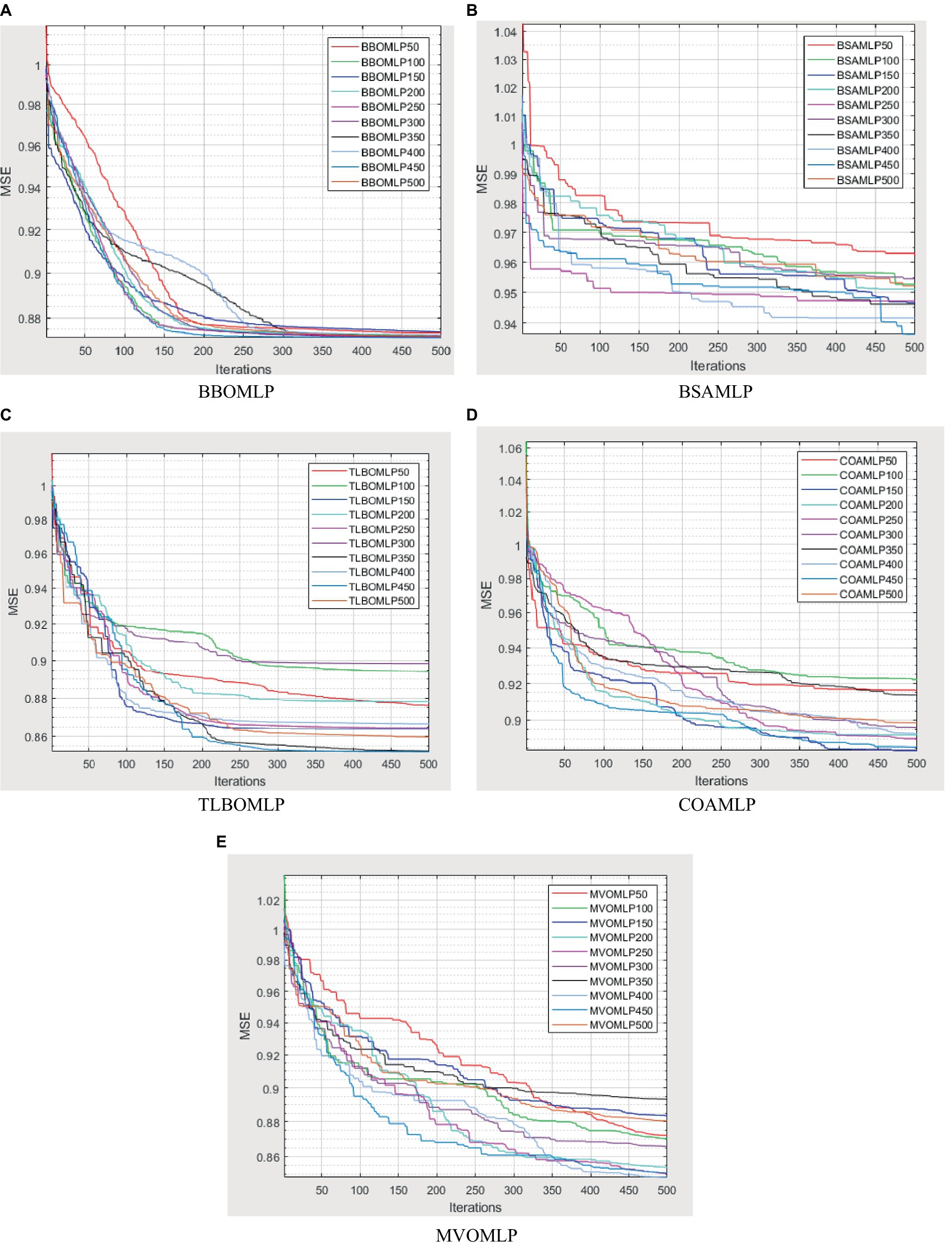
Figure 7. Variation of mean squared error versus iterations for the (A) BBOMLP, (B) BSAMLP, (C) TLBOMLP, (D) COAMLO, and (E) MVOMLP.

In addition, it should be noted that each algorithm exhibits ten unique subtleties, corresponding to population sizes of 50, 100, 150, 200, 250, 300, 350, 400, 450, and 500. The ideal population size is determined by selecting the population size that yields the smallest mean squared error (MSE). This ensures that the swarm working on the task operates with the most acceptable size. Regarding their optimization behavior, the mean squared error (MSE) values, specifically the convergence curves, of several high-ranking structures.

The evaluation of the overall efficacy of categorization may be conducted by using a metric called the receiver operating characteristic curve (ROC). The false-positive rate (FPR) corresponds to the error rate attributed to the minority class and is graphed on the X-axis of the receiver operating characteristic (ROC) curve. The Y-axis is indicative of the true positive rate (TPR). The classifier’s efficacy is considered to be higher when the receiver operating characteristic (ROC) curve is positioned closer to the top left corner. This observation suggests an inverse relationship between the magnitude of the Y variable and the magnitude of the X variable. However, the receiver operating characteristic (ROC) curve has a limitation that hinders its ability to be used for quantitative evaluation of the classifier’s efficacy. Consequently, the AUC value, which refers to the area under the receiver operating characteristic (ROC) curve, was used to evaluate the efficacy of the categorisation. The trade-off between recall and accuracy is seen in the ROC curves presented in Figures 8–12. As a result, the investigator has the capacity to manipulate the metrics of false positive and genuine positive (46, 47). A conventional confusion matrix was used to provide a comprehensive overview of the associations between false positives, true positives, false negatives, and true negatives. The data may be compared to the various areas under the curves generated from the receiver operating characteristic (ROC) curves, as shown in Tables 2–6, for population numbers ranging from 50 to 500. Upon comparing all five strategies, it is evident from the curves that the teaching-learning-based optimization (MVO) method has the best degree of efficacy (Figures 8–11, 13).

Figure 8

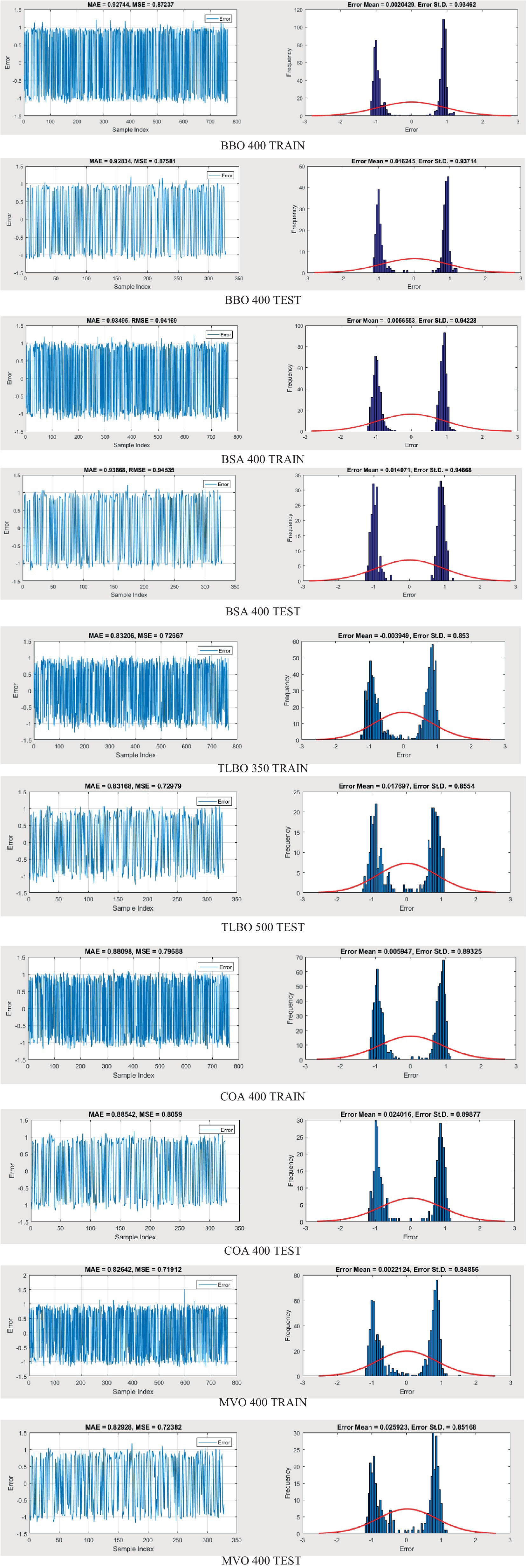
Figure 8. ROC amount for BSAMLP.

Figure 9

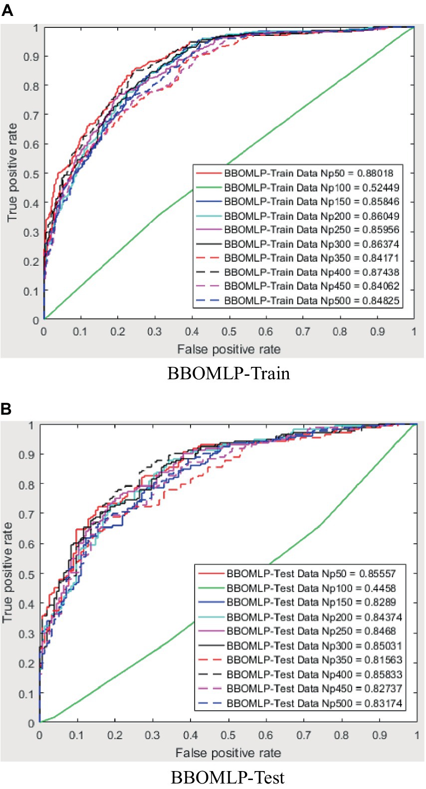
Figure 9. ROC amount for TLBOMLP.

Figure 10

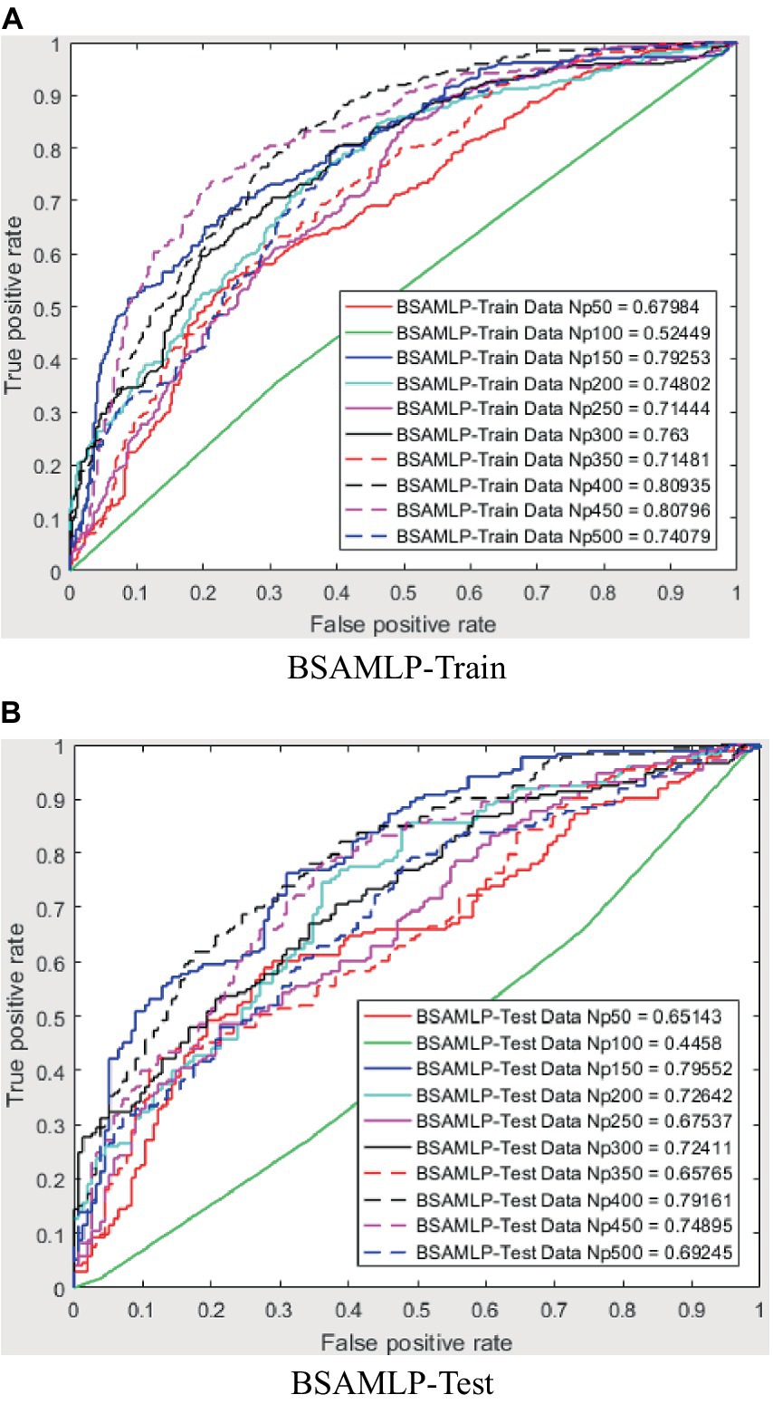
Figure 10. ROC amount for COAMLP.

Figure 11

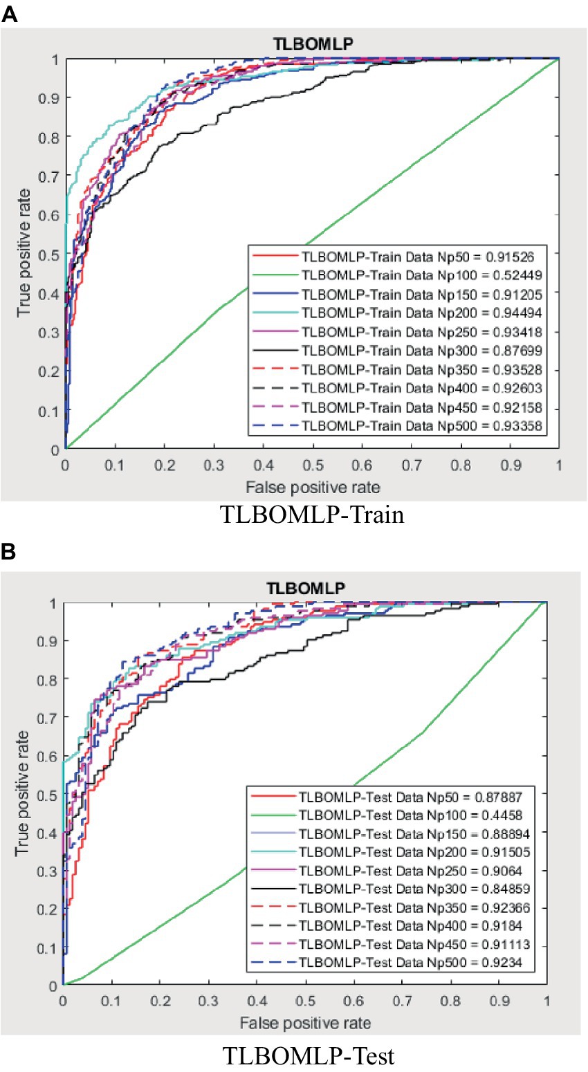
Figure 11. ROC amount for MVOMLP.

Figure 12

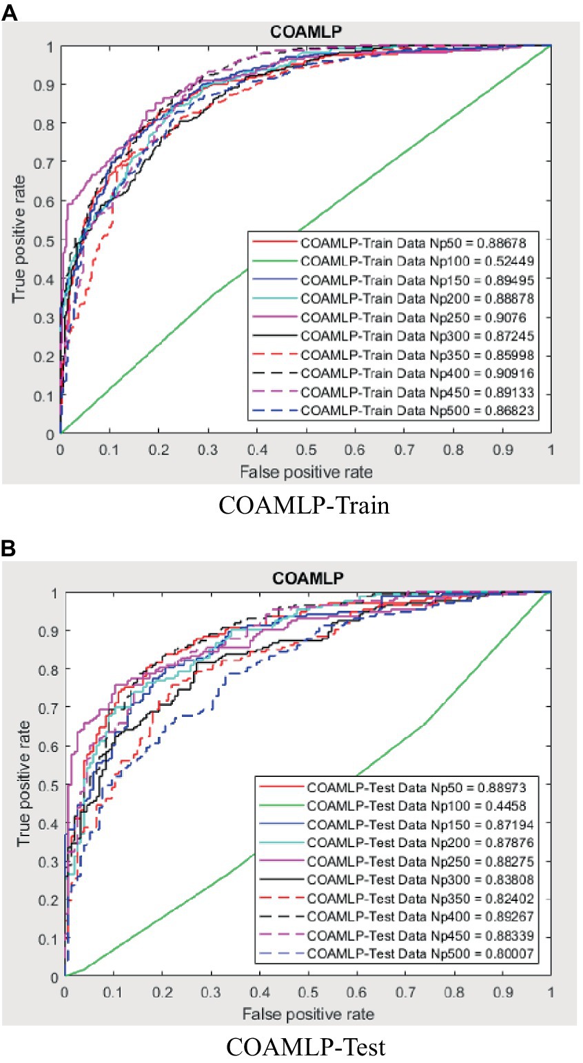
Figure 12. Error frequency and values to evaluates the efficacy of the applied models.

Table 2

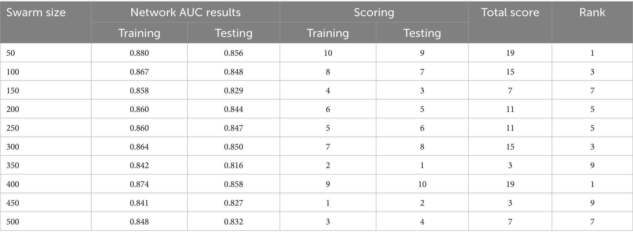
Table 2. AUC BBO.

Table 3

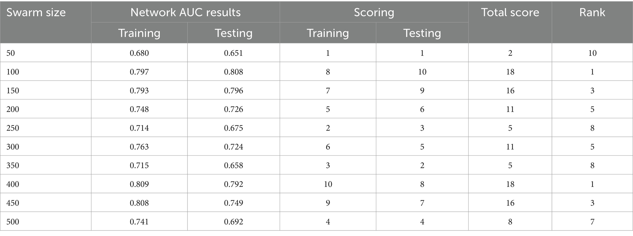
Table 3. AUC BSA.

Table 4

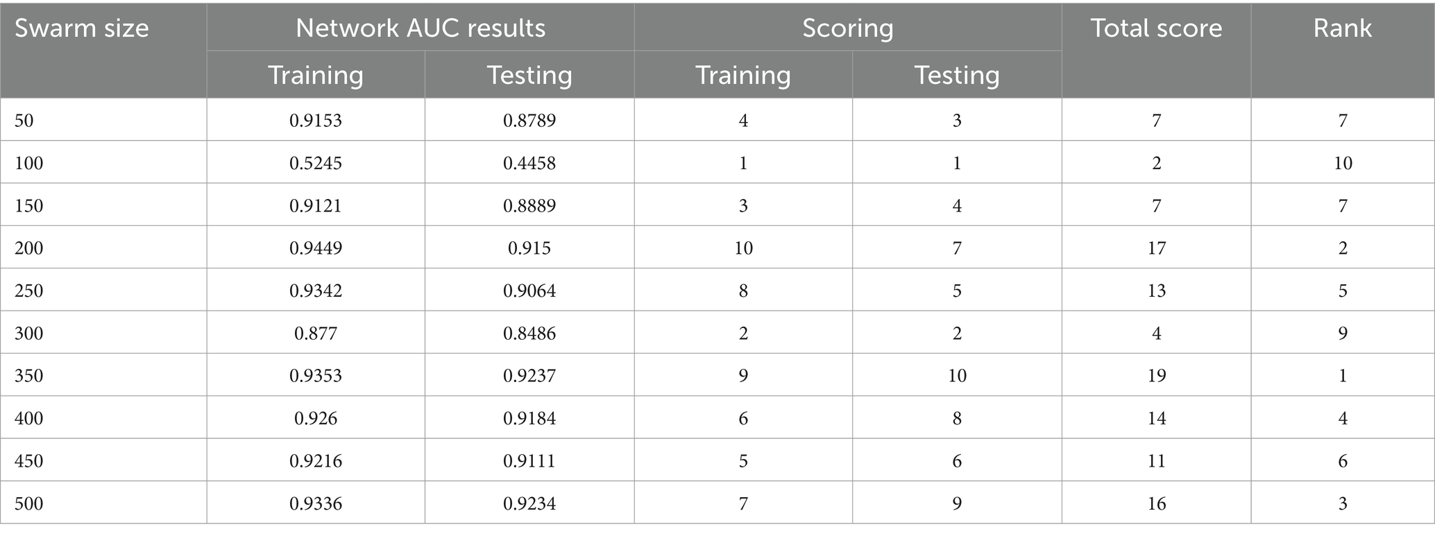
Table 4. AUC TLBO.

Table 5

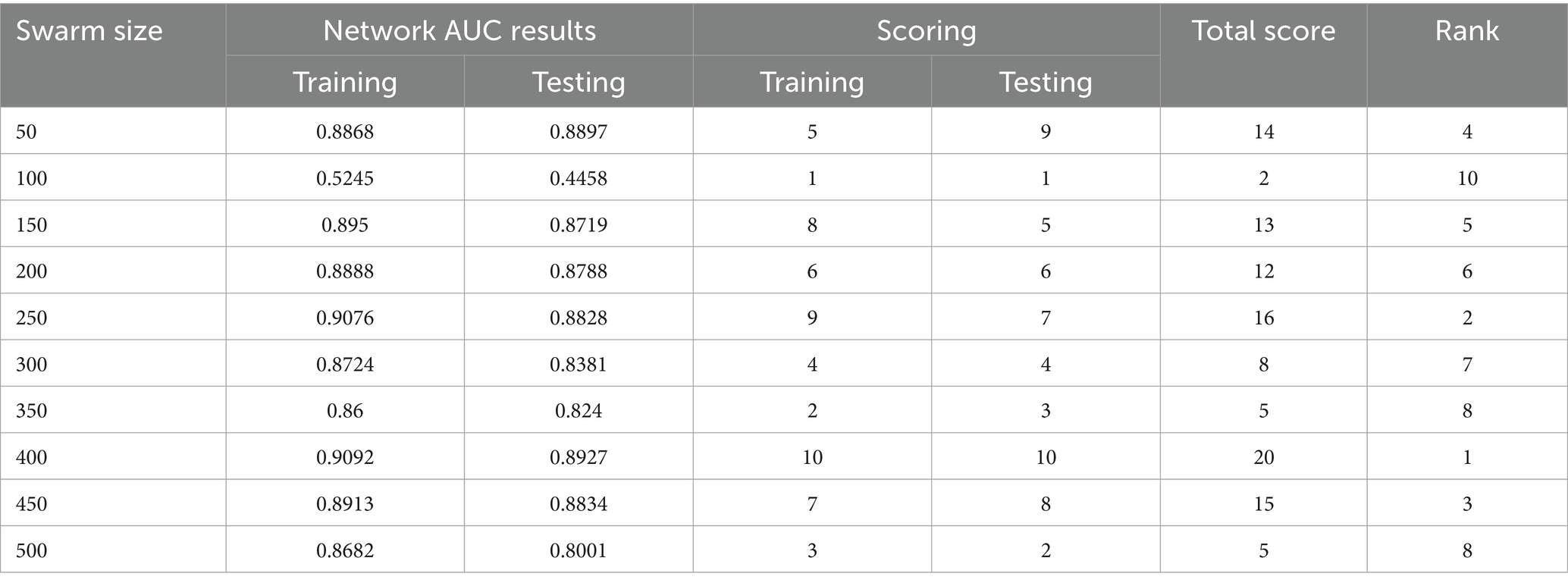
Table 5. AUC COA.

Table 6

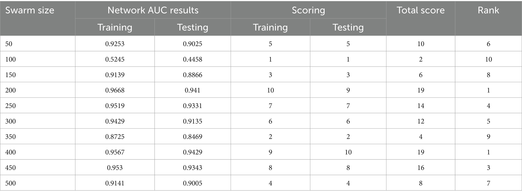
Table 6. AUC MVO.

Figure 13

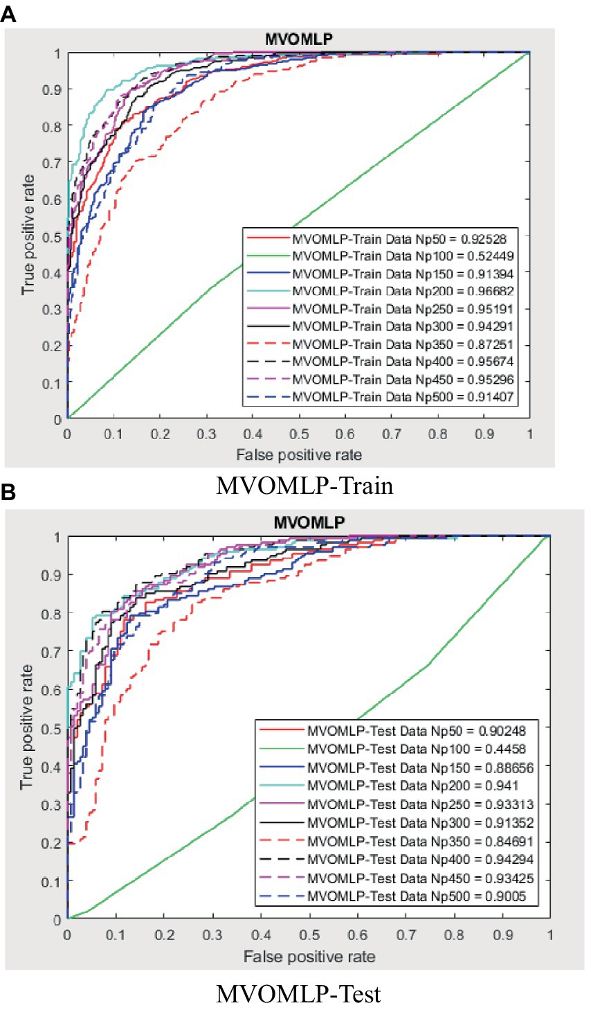
Figure 13. ROC amount for BBOMLP.

4.1 AUC optimization

The use of the universal binary classification metric, often referred to as area under curve (AUC), is a prevalent practice seen across several academic disciplines. The evaluation of a credit scoring system might also include the use of more specific indicators. The findings of the three methods based on the AUC values are shown in Tables 2–6. The training dataset consisted of 80 percent of the information in the dataset, while the remaining 20 percent was allocated for testing purposes. Upon implementing the BBO-MLP algorithm on the given dataset, we achieved accuracy scores of 87.4 and 85.8% for the training and test datasets, respectively. Upon implementation of the BSA-MLP method on our dataset, the accuracy values obtained for the training and test datasets were 80.9 and 79.2% respectively. The TLBO-MLP approach achieved training AUC values of 93.53% and testing AUC values of 92.37%. On the other hand, the COA-MLP method produced training AUC values of 90.92% and testing AUC values of 89.27%. Ultimately, the most effective strategy is determined to be the MVO-MLP method, which exhibits the greatest AUC values of 95.67 and 94.29% throughout the training and testing phases, respectively (Tables 2–6).

4.2 Error assessment

This section evaluates the efficacy of various models by comparing their yield to the goal values, with a focus on error values and performance metrics during both training and testing phases.

Figures 12 illustrate the results of the training phase, highlighting the variations between each output combination. The training error values for the biography-based optimization (BBO-MLP), backtracking search algorithm (BSA-MLP), teaching-learning-based optimization (TLBO-MLP), and cuckoo optimization algorithm (COA-MLP) models range between (0.0020429, 0.93462), (−0.0056553, 0.94228), (−0.003949, 0.853), and (0.005947, 0.89325), respectively. For the testing phase, these error values are (0.016245, 0.93714), (0.014071, 0.94668), (0.017697, 0.8554), and (0.024016, 0.89877), respectively. The multi-verse optimization (MVO-MLP) model demonstrates the lowest error values in both training and testing stages, with ranges of (0.0022124, 0.84856) and (0.025923, 0.85168), respectively. Moreover, the mean absolute error (MAE) values for the BBO-MLP, BSA-MLP, TLBO-MLP, COA-MLP, and MVO-MLP methods in the training stage are (0.92744, 0.93945, 0.83206, 0.88098, and 0.82642) and in the testing stage are (0.92834, 0.93868, 0.83168, 0.88542, and 0.82928). The mean squared error (MSE) values for these methods in the training stage are (0.87237, 0.94169, 0.72667, 0.79688, and 0.71912) and in the testing stage are (0.87581, 0.94535, 0.72979, 0.8059, and 0.72382). These results indicate that the MVO-MLP method outperforms the other methods, showing better accuracy in predicting crude oil prices. The lower error values in both training and testing phases, along with superior MAE and MSE metrics, suggest that the MVO-MLP model has a higher precision and reliability. This demonstrates the effectiveness of the multi-verse optimization algorithm in enhancing the performance of ANNs for complex prediction tasks like crude oil price forecasting.

5 Conclusion

This paper aimed to investigate, analyze, and develop five machine-learning algorithm to accurately predict successful trading in the West Texas Intermediate crude oil cash market. According to the results of this research, using five different categorization approaches [biography-based optimization (BBO), backtracking search algorithm (BSA), and teaching-learning-based optimization (TLBO), cuckoo optimization algorithm (COA), and multi-verse optimization algorithm (MVO)]. The multiverse optimization approach yielded the maximum AUC score possible, which was 0.9567 and 0.9429 in raining and testing stages, respectively. The other four methods also show a high value of AUC (greater than 0.8). The values of (0.874 and 0.792), (0.809 and 0.792), (0.9353 and 0.9237), and (0.9092 and 0.8927) obtained for AUC in training and testing stages, for BBO-MLP, BSA-MLP, TLBO-MLP, and COA-MLP methods, respectively. This number was used to determine the crude oil cash. Therefore, the teaching-learning-based optimization strategy can be used for the categorization of crude oil cash. Due to the fact that the algorithm places certain non-defaulters in the default category, we may wish to investigate this problem deeper in order to improve the model’s ability to anticipate prediction of crude oil price. However, this strategy has many drawbacks. Numerous variables (supply and demand, supplier competition, replacement with other energy sources, technological advancement, local economics, deregulatory activities, globalization, and even political instability and conflicts) are known to influence the price of crude oil. In addition, the decomposition results rely on the selection of parameters, but the methodology fails to give a theoretical economic foundation for the decomposition rules. The integrated models are tested on historical data from the WTI crude oil cash market. Preliminary results indicate significant improvements in prediction accuracy when optimization algorithms are utilized in conjunction with ANNs. Detailed comparative analysis highlights the strengths and weaknesses of each approach, providing insights into their applicability in real-world trading scenarios. The study demonstrates that the integration of optimization algorithms with ANNs can lead to superior predictive performance. Each algorithm contributes uniquely to the training process, offering diverse strategies for escaping local optima and enhancing generalization capabilities. This research underscores the potential of hybrid models combining ANNs with advanced optimization algorithms in predicting successful trades in the WTI crude oil cash market. Future work will explore the integration of additional algorithms and the application of these models to other financial markets.

Data availability statement

The original contributions presented in the study are included in the article/Supplementary material, further inquiries can be directed to the corresponding authors.

Author contributions

EB: Writing – original draft. AM: Writing – original draft. SJ: Writing – original draft. MG: Writing – original draft. GR: Writing – original draft. ST: Writing – original draft. SR: Writing – original draft. MK: Writing – original draft.

Funding

The author(s) declare that no financial support was received for the research, authorship, and/or publication of this article.

Conflict of interest

The authors declare that the research was conducted in the absence of any commercial or financial relationships that could be construed as a potential conflict of interest.

Publisher’s note

All claims expressed in this article are solely those of the authors and do not necessarily represent those of their affiliated organizations, or those of the publisher, the editors and the reviewers. Any product that may be evaluated in this article, or claim that may be made by its manufacturer, is not guaranteed or endorsed by the publisher.

Supplementary material

The Supplementary material for this article can be found online at: https://www.frontiersin.org/articles/10.3389/fams.2024.1376558/full#supplementary-material

References

1. Serletis, A, and Rosenberg, AA. The Hurst exponent in energy futures prices. Physica A. (2007) 380:325–32. doi: 10.1016/j.physa.2007.02.055

Crossref Full Text | Google Scholar

2. Tabak, BM, and Cajueiro, DO. Are the crude oil markets becoming weakly efficient over time? A test for timevarying long-range dependence in prices and volatility. Energy Econ. (2007) 29:28–36. doi: 10.1016/j.eneco.2006.06.007

Crossref Full Text | Google Scholar

3. Alvarez-Ramirez, J, Alvarez, J, and Rodriguez, E. Short-term predictability of crude oil markets: a detrended fluctuation analysis approach. Energy Econ. (2008) 30:2645–56. doi: 10.1016/j.eneco.2008.05.006

Crossref Full Text | Google Scholar

4. Wang, Y, and Liu, L. Is WTI crude oil market becoming weakly efficient over time?: new evidence from multiscale analysis based on detrended fluctuation analysis. Energy Econ. (2010) 32:987–92. doi: 10.1016/j.eneco.2009.12.001

Crossref Full Text | Google Scholar

5. He, L-Y, and Chen, S-P. Are crude oil markets multifractal? Evidence from MF-DFA and MF-SSA perspectives. Physica A. (2010) 389:3218–29. doi: 10.1016/j.physa.2010.04.007

Crossref Full Text | Google Scholar

6. Gu, R, Chen, H, and Wang, Y. Multifractal analysis on international crude oil markets based on the multifractal detrended fluctuation analysis. Physica A. (2010) 389:2805–15. doi: 10.1016/j.physa.2010.03.003

Crossref Full Text | Google Scholar

7. Alvarez-Ramirez, J, Alvarez, J, and Solis, R. Crude oil market efficiency and modeling: insights from the multiscaling autocorrelation pattern. Energy Econ. (2010) 32:993–1000. doi: 10.1016/j.eneco.2010.04.013

Crossref Full Text | Google Scholar

8. Moshiri, S, and Foroutan, F. Forecasting nonlinear crude oil futures prices. Energy J. (2006) 27:81–96. doi: 10.5547/ISSN0195-6574-EJ-Vol27-No4-4

Crossref Full Text | Google Scholar

9. Wang, S, Yu, L, and Lai, KK. Crude oil price forecasting with TEI@ I methodology. J Syst Sci Complex. (2005) 18:145.

Google Scholar

10. Jovanovic, L, Jovanovic, D, Bacanin, N, Jovancai Stakic, A, Antonijevic, M, Magd, H, et al. Multi-step crude oil price prediction based on LSTM approach tuned by salp swarm algorithm with disputation operator. Sustainability. (2022) 14:14616. doi: 10.3390/su142114616

Crossref Full Text | Google Scholar

11. Chen, ZY . A computational intelligence hybrid algorithm based on population evolutionary and neural network learning for the crude oil spot price prediction. Int J Comput Intell Syst. (2022) 15:68. doi: 10.1007/s44196-022-00130-4

Crossref Full Text | Google Scholar

12. Sohrabi, P, Dehghani, H, and Rafie, R. Forecasting of WTI crude oil using combined ANN-Whale optimization algorithm. Energy Sources B. (2022) 17:2083728. doi: 10.1080/15567249.2022.2083728

Crossref Full Text | Google Scholar

13. Das, AK, Mishra, D, Das, K, Mallick, PK, Kumar, S, Zymbler, M, et al. Prophesying the short-term dynamics of the crude oil future price by adopting the survival of the fittest principle of improved grey optimization and extreme learning machine. Mathematics. (2022) 10:1121. doi: 10.3390/math10071121

Crossref Full Text | Google Scholar

14. Gulati, K, Gupta, J, Rani, L, and Kumar Sarangi, P. (2022). Crude oil prices predictions in India using machine learning based hybrid model. 2022 10th International Conference on Reliability, Infocom Technologies and Optimization (Trends and Future Directions) (ICRITO). IEEE. 1–6).

Google Scholar

15. Xie, W, Yu, L, Xu, S, and Wang, S. (2006). A new method for crude oil price forecasting based on support vector machines. International Conference on Computational Science. Berlin: Springer.

Google Scholar

16. Silvapulle, P, and Moosa, IA. The relationship between spot and futures prices: evidence from the crude oil market. J Futures Mark. (1999) 19:175193

Google Scholar

17. Zhao, Y, Maria Joseph, AJJ, Zhang, Z, Ma, C, Gul, D, Schellenberg, A, et al. Deterministic snap-through buckling and energy trapping in axially-loaded notched strips for compliant building blocks. Smart Mater Struct. (2020) 29:02LT03. doi: 10.1088/1361-665X/ab6486

Crossref Full Text | Google Scholar

18. Chen, S, Zhang, H, Wang, L, Yuan, C, Meng, X, Yang, G, et al. Experimental study on the impact disturbance damage of weakly cemented rock based on fractal characteristics and energy dissipation regulation. Theor Appl Fract Mech. (2022) 122:103665. doi: 10.1016/j.tafmec.2022.103665

Crossref Full Text | Google Scholar

19. Brooks, C, Rew, AG, and Ritson, S. A trading strategy based on the lead-lag relationship between the spot index and futures contract for the FTSE 100. Int J Forecast. (2001) 17:31–44. doi: 10.1016/S0169-2070(00)00062-5

Crossref Full Text | Google Scholar

20. Bopp, AE, and Sitzer, S. Are petroleum futures prices good predictors of cash value? J Futures Mark. (1987) 19:705–19. doi: 10.1002/fut.3990070609

Crossref Full Text | Google Scholar

21. Chan, K . A further analysis of the lead-lag relationship between the cash market and stock index futures market. Rev Financ Stud. (1992) 5:123–52. doi: 10.1093/rfs/5.1.123

Crossref Full Text | Google Scholar

22. Coppola, A . Forecasting oil price movements: exploiting the information in the futures market. J Futures Mark. (2008) 28:34–56. doi: 10.1002/fut.20277

Crossref Full Text | Google Scholar

23. Abosedra, S, and Baghestani, H. On the predictive accuracy of crude oil futures prices. Energy Policy. (2004) 32:1389–93. doi: 10.1016/S0301-4215(03)00104-6

Crossref Full Text | Google Scholar

24. McNelis, PD . Neural networks in finance: gaining predictive edge in the market. Elsevier press: Academic Press. (2005).

Google Scholar

25. Smith, M . Neural networks for statistical modeling. Thomson Learning. USA: John Wiley Sons Inc. (1993).

Google Scholar

26. Refenes, A-P . Neural networks in the capital markets. New York-USA: John Wiley & Sons, Inc. (1994).

Google Scholar

27. Moayedi, H, Varamini, N, Mosallanezhad, M, Kok Foong, L, and Nguyen le, B. Applicability and comparison of four nature-inspired hybrid techniques in predicting driven piles’ friction capacity. Transp Geotech. (2022) 37:100875. doi: 10.1016/j.trgeo.2022.100875

Crossref Full Text | Google Scholar

28. Zhao, Y, and Foong, LK. Predicting electrical power output of combined cycle power plants using a novel artificial neural network optimized by electrostatic discharge algorithm. Measurement. (2022) 198:111405. doi: 10.1016/j.measurement.2022.111405

Crossref Full Text | Google Scholar

29. Zhao, Y, Yan, Q, Yang, Z, Yu, X, and Jia, B. A novel artificial bee colony algorithm for structural damage detection. Adv Civ Eng. (2020) 2020:1–21. doi: 10.1155/2020/3743089

Crossref Full Text | Google Scholar

30. Zhao, Y, Hu, H, Song, C, and Wang, Z. Predicting compressive strength of manufactured-sand concrete using conventional and metaheuristic-tuned artificial neural network. Measurement. (2022) 194:110993. doi: 10.1016/j.measurement.2022.110993

Crossref Full Text | Google Scholar

31. Energy Information Administration (U.S.) . Annual energy outlook 2011: with projections to 2035. US department of energy, Washington, USA: Government Printing Office (2011).

Google Scholar

32. Zhao, Y, Bai, C, Xu, C, and Foong, LK. Efficient metaheuristic-retrofitted techniques for concrete slump simulation. Smart Struct Syst. (2021) 27:745–59. doi: 10.12989/sss.2021.27.5.745

Crossref Full Text | Google Scholar

33. Yan, B, Ma, C, Zhao, Y, Hu, N, and Guo, L. Geometrically enabled soft electroactuators via laser cutting. Adv Eng Mater. (2019) 21:1900664. doi: 10.1002/adem.201900664

Crossref Full Text | Google Scholar

34. Liu, B, Tian, M, Zhang, C, and Li, X. Discrete biogeography based optimization for feature selection in molecular signatures. Mol Inform. (2015) 34:197–215. doi: 10.1002/minf.201400065

PubMed Abstract | Crossref Full Text | Google Scholar

35. Zhao, Y, Hu, H, Bai, L, Tang, M, Chen, H, and Su, D. Fragility analyses of bridge structures using the logarithmic piecewise function-based probabilistic seismic demand model. Sustainability. (2021) 13:7814. doi: 10.3390/su13147814

Crossref Full Text | Google Scholar

36. Civicioglu, P . Backtracking search optimization algorithm for numerical optimization problems. Appl Math Comput. (2013) 219:8121–44. doi: 10.1016/j.amc.2013.02.017

Crossref Full Text | Google Scholar

37. Wu, P, Liu, A, Fu, J, Ye, X, and Zhao, Y. Autonomous surface crack identification of concrete structures based on an improved one-stage object detection algorithm. Eng Struct. (2022) 272:114962. doi: 10.1016/j.engstruct.2022.114962

Crossref Full Text | Google Scholar

38. Rao, RV, Savsani, VJ, and Vakharia, D. Teaching-learning-based optimization: an optimization method for continuous non-linear large scale problems. Inf Sci. (2012) 183:1–15. doi: 10.1016/j.ins.2011.08.006

Crossref Full Text | Google Scholar

39. Rao, RV, Savsani, VJ, and Vakharia, D. Teaching-learning-based optimization: a novel method for constrained mechanical design optimization problems. Comput Aided Des. (2011) 43:303–15. doi: 10.1016/j.cad.2010.12.015

Crossref Full Text | Google Scholar

40. Zhao, Y, and Wang, Z. Subset simulation with adaptable intermediate failure probability for robust reliability analysis: an unsupervised learning-based approach. Struct Multidiscip Optim. (2022) 65:1–22. doi: 10.1007/s00158-022-03260-7

Crossref Full Text | Google Scholar

41. Bakhshi, M, Karkehabadi, A, and Razavian, SB. (2024). Revolutionizing medical diagnosis with novel teaching-learning-based optimization. 2024 International Conference on Emerging Smart Computing and Informatics (ESCI). IEEE. 1–6.

Google Scholar

42. Sasani, F, Mousa, R, Karkehabadi, A, Dehbashi, S, and Mohammadi, A. (2023). TM-vector: a novel forecasting approach for market stock movement with a rich representation of twitter and market data. arXiv. Available at: https://doi.org/10.48550/arXiv.2304.02094. [Epub ahead of preprint]

Google Scholar

43. Zhao, Y. , H. Moayedi, M. Bahiraei, and L. K. Foong, Employing TLBO and SCE for optimal prediction of the compressive strength of concrete. Smart Struct Syst. (2020). 26: p. 753–763, doi: 10.12989/sss.2020.26.6.753

Crossref Full Text | Google Scholar

44. Rao, R.V., and Savsani, V.J., Mechanical design optimization using advanced optimization techniques. (2012).

Google Scholar

45. Rajabioun, R . Cuckoo optimization algorithm. Appl Soft Comput. (2011) 11:5508–18. doi: 10.1016/j.asoc.2011.05.008

Crossref Full Text | Google Scholar

46. Steenackers, A, and Goovaerts, M. A credit scoring model for personal loans. Insur Math Econ. (1989) 8:31–4. doi: 10.1016/0167-6687(89)90044-9

Crossref Full Text | Google Scholar

47. Sun, L, and Shenoy, PP. Using Bayesian networks for bankruptcy prediction: some methodological issues. Eur J Oper Res. (2007) 180:738–53. doi: 10.1016/j.ejor.2006.04.019

Crossref Full Text | Google Scholar