 Abdullah Hasan Hassan
 Dipo Aldila
 Muhamad Hifzhudin Noor Aziz
- 1Department of Mathematics, Faculty of Mathematics and Natural Sciences, Universitas Indonesia, Depok, Indonesia
- 2Institute of Mathematical Sciences, Faculty of Science, Universiti Malaya, Kuala Lumpur, Malaysia
This study presents a comprehensive analysis of the transmission dynamics of monkeypox, considering contaminated surfaces using a deterministic mathematical model. The study begins by calculating the basic reproduction number and the stability properties of equilibrium states, specifically focusing on the disease-free equilibrium and the endemic equilibrium. Our analytical investigation reveals the occurrence of a forward bifurcation when the basic reproduction number equals unity, indicating a critical threshold for disease spread. The non-existence of backward bifurcation indicates that the basic reproduction number is the single endemic indicator in our model. To further understand the dynamics and control strategies, sensitivity analysis is conducted to identify influential parameters. Based on these findings, the model is reconstructed as an optimal control problem, allowing for the formulation of effective control strategies. Numerical simulations are then performed to assess the impact of these control measures on the spread of monkeypox. The study contributes to the field by providing insights into the optimal control and stability analysis of monkeypox transmission dynamics. The results emphasize the significance of contaminated surfaces in disease transmission and highlight the importance of implementing targeted control measures to contain and prevent outbreaks. The findings of this research can aid in the development of evidence-based strategies for mitigating the impact of monkeypox and other similar infectious diseases.
1 Introduction
The global outbreak of monkeypox in May 2022 has highlighted the significant public health risks associated with zoonotic diseases [1]. Monkeypox, caused by the monkeypox virus, primarily spreads to humans through contact with infected animals, but human-to-human transmission can also occur through various routes [2, 3]. Contaminated surfaces play a crucial role in the transmission of diseases. Studies indicate that viral transmission can take place through contaminated surfaces, and mounting evidence underscores the pivotal role of contaminated fomites or surfaces in the spread of viral diseases [4]. Specifically, the environmental viral load significantly influences the transmission of the monkeypox virus, with direct contact with contaminated items or materials emerging as a major contributing factor to its spread [5]. The disease manifests in distinct phases, including an incubation period, a prodromal phase, and an eruptive stage characterized by skin lesions [2, 6]. The ongoing monkeypox outbreak has become a public health emergency of global concern, with over 63,000 cases reported, including its spread to locations such as the United Kingdom [7, 8]. This outbreak poses a strain on healthcare systems already dealing with the COVID-19 pandemic [9]. Although monkeypox cases are typically mild, at-risk groups such as children, gravid women, and individuals with compromised immune systems may experience severe cases [10, 11]. Historically, monkeypox outbreaks have been prevalent in marginalized communities in Africa, where the disease became endemic [12–14]. Concerns have been raised due to waning immunity resulting from the discontinuation of smallpox vaccination and the evolving epidemiology of the virus [15, 16]. To effectively address the monkeypox outbreak, it is crucial to develop robust disease modeling strategies for public health planning and response.
Previously, there has been limited focus on monkeypox, resulting in a lack of understanding of the disease's transmission dynamics. However, a few numbers of studies have made efforts to employ mathematical modeling techniques to gain insights into the monkeypox virus's dynamics. Mathematical modeling has been studied in Al-Shomrani et al. [17] to analyze the interaction between humans and animals in relation to the Monkeypox virus, while Okyere and Ackora-Prah[18] explores the mechanism of human transmission of the virus through a mathematical study. The authors in Peter et al. [19] investigated the transmission dynamics of the monkeypox virus and found that isolating infected individuals in the human population effectively reduces disease transmission. Alharbi et al. [20] explored the effectiveness of treatment and vaccination interventions as containment measures for monkeypox. In a study by Michael et al. [21], the authors examined a mathematical model for monkeypox that incorporated surveillance as a control measure. Additional valuable contributions can be found in El-Mesady et al. [22], Alshehri and Ullah [23], and Alzubaidi et al. [24]. According to the existing literature, it is evident that further research and exploration are necessary to gain a deeper understanding of the phenomenon of monkeypox. This study aims to investigate the dynamics of monkeypox transmission and its control in humans by employing a classical and deterministic model that incorporates contaminated surfaces as a separate compartment.
In our study, we present a novel contribution to the field by adopting a deterministic approach, distinguishing our study from previous studies conducted by Addai et al. [5] and Li et al. [25], who utilized the Caputo fractional derivative. Furthermore, while Madubueze et al. [26] employed a deterministic model and made commendable progress, our study extends beyond by conducting more in-depth analyses in optimal control and numerical simulations for the proposed strategies. Additionally, our research sets itself apart from the study by Alshehri et al. [23], who also employed a deterministic model by incorporating an exposed population variable into our model and conducting a comprehensive cost-effectiveness analysis for the implemented strategies. Our strong emphasis on these aspects showcases the distinctive contributions and advancements made in our study compared to the existing literature.
The subsequent sections of this article are outlined in the following manner: In Section 2, we explain the construction of the mathematical model. Next, Section 3 focuses on analyzing the model, including the disease-free equilibrium, basic reproduction number, endemic equilibrium, and global stability. We conduct a bifurcation analysis in Section 4. Section 5 presents a sensitivity analysis of the model. Section 6, explores an optimal control problem, including its characterization, simulation, and discussion. Finally, we conclude the article by summarizing the key findings in Section 7.
2 Model construction
In this section, we present the construction of our mathematical model for the optimal control and stability analysis of monkeypox transmission dynamics, considering the impact of contaminated surfaces. In developing the model, an assumption is made that the population of humans (N) remains constant over a period of time. The model is developed based on compartmentalization, where individuals are classified into different compartments representing their disease status. We consider the following compartments: susceptible (S), exposed (E), infectious (I), recovered (R), and contaminated surfaces (C). The explanations of the model construction for each compartment are constructed using Figure 1 and given as follows:
• Susceptible (S). This compartment represents individuals who are susceptible to contracting monkeypox. They have not been exposed to the virus and can become infected if they come into contact with infectious individuals or contaminated surfaces. The rate of change in the susceptible compartment is determined by multiple factors. First, the birth rate of the human population (Λh) contributes to the increase in the number of susceptible individuals. Second, the term represents the combined effect of virus transmission from infectious individuals (I) and contaminated surfaces (C) to susceptible individuals, where βh and βc represent the transmission rate of monkeypox through contact of human to other human or contaminated surfaces, respectively. This term signifies the rate at which susceptible individuals become infected. In addition, it is important to note that the natural mortality rate denoted by (μh) applies to all compartments, including the infected and recovered. This rate contributes to the decrease in the respective populations due to non-disease-related causes.
• Exposed (E). The exposed compartment represents individuals who have been exposed to the monkeypox virus but are not yet infectious. During this period, the virus is incubating within their bodies, and they do not exhibit symptoms or pose an immediate risk of transmission. However, they can potentially transmit the virus to susceptible individuals or contaminated surfaces. The rate of change in the exposed compartment depends on various factors. The term represents the rate at which exposed individuals become infected, considering virus transmission from infectious individuals (I) and contaminated surfaces (C). Additionally, γE accounts for the transition from the exposed to the infectious stage, where γ represents the transition rate due to infection progression. This term represents the rate at which exposed individuals progress to the infectious compartment.
• Infectious (I). The infectious compartment consists of individuals who have become infectious and can spread the monkeypox virus to susceptible individuals or contaminated surfaces. They may exhibit symptoms of the disease and contribute to the transmission dynamics. The rate of change in the infectious compartment is influenced by several factors. First, γE represents the rate at which exposed individuals progress to the infectious stage, reflecting the transition from the exposed compartment to the infectious compartment. Moreover, γ0I signifies the rate at which infectious individuals recover and transition to the recovered compartment, where γ0 represents the recovery rate from monkeypox.
• Recovered (R). This compartment represents individuals who have recovered from the monkeypox infection and developed immunity. The rate of change in the recovered compartment is primarily determined by the rate at which infectious individuals recover and transition to the recovered compartment, denoted as γ0I.
• Contaminated surfaces (C). The contaminated surfaces compartment represents surfaces or environments that have been contaminated by the monkeypox virus. These surfaces can act as sources of infection if individuals come into contact with them. The virus can persist on these surfaces and potentially contribute to the transmission of monkeypox. The rate of change in the contaminated surfaces compartment is influenced by two main factors. First, αI denotes the rate at which infectious individuals contaminate surfaces, indicating the rate at which the virus is deposited on surfaces. Second, μpC represents the cleaning rate or decay rate of the virus on contaminated surfaces, signifying the rate at which the virus is removed or becomes inactive on surfaces.
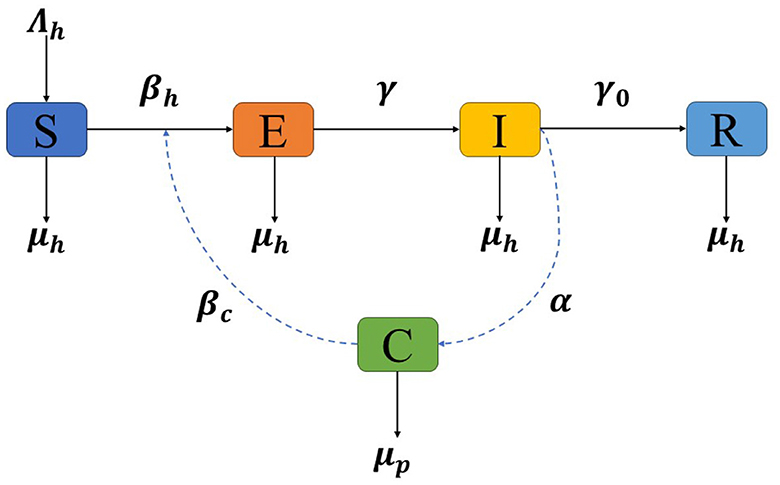
Figure 1. Transmission diagram depicting the spread of the disease in the model.
The model can be represented by the following set of differential equations:
The initial conditions of the model (Equation 1) are non-negative:
All parameters in the system are positive. The specific values of these parameters and their descriptions are provided in Table 1. Before doing additional analysis on the model, it is essential to ensure that the solutions of system (Equation 1) exhibit both positivity and boundedness. These properties are stated in the following theorems.
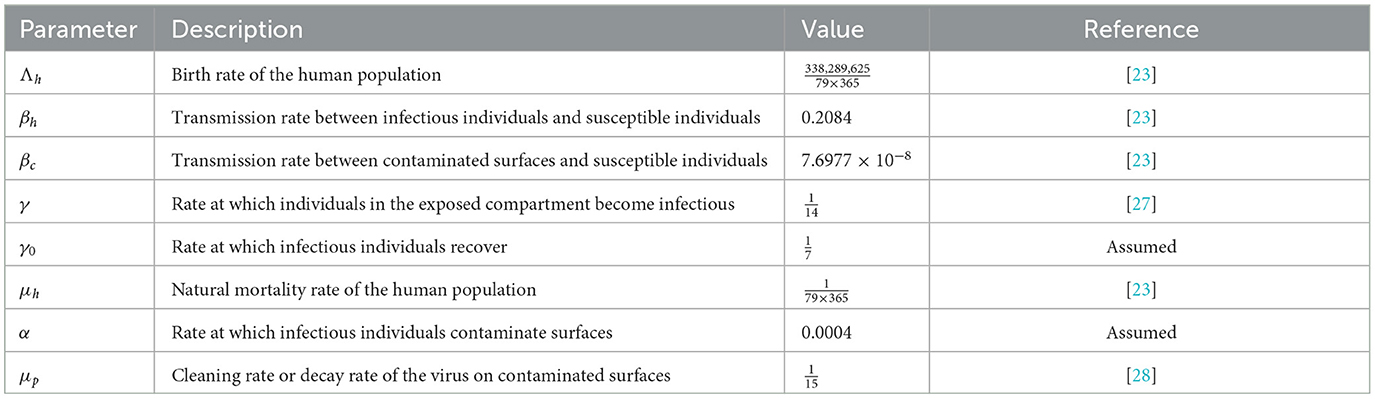
Table 1. Parameter descriptions and values for the basic model (1).
Theorem 1. Given non-negative initial conditions (Equation 2), every solution (S, E, I, R, C) of model (Equation 1) is positive for all t ≥ 0.
Proof. In the boundary region of , we have system (Equation 1) equals to:
The computation above shows that on the boundary planes of the non-negative of , all of the rates are non-negative. Consequently, all of the vector field direction is inward from the boundary planes. As a result, initiating the system from non-negative initial conditions ensures that all solutions remain positive.
Theorem 2. The solutions of model (Equation 1) are bounded in the region
Proof. Combining the first four equations within the model (Equation 1) yields an equation that describes the overall population as follows:
By applying the integrating factor method using , it can be established that N(t) satisfies:
If we take the limit as t → ∞, we have . If the initial condition is larger than , then the solution will monotonically decrease and tends to . If , then the solution will monotonically increase and tends to . On the other hand, if , then the solution will remain constant at . Hence, we have .
For the variable C, since I ≤ N, we got
Moreover, employing the integrating factor method with , we get
With t → ∞, . Hence, the theorem is proven.
To facilitate further analysis of the model, we apply scaling techniques to normalize the variables. By introducing the scaling variables , and , where N represents the total population size, we can express the model in dimensionless form. Additionally, we redefine the transmission rate of contaminated surfaces as βp = βcN. Utilizing the relationship s = 1 − e − i − r, the final model is obtained:
In this transformed form, all variables and parameters in model (Equation 3) are dimensionless, enabling a more convenient analysis of the model's behavior and stability properties.
3 Analysis of the model
3.1 The monkeypox-free equilibrium and the basic reproduction number
The monkeypox-free equilibrium is a crucial state in the analysis of the proposed model. It represents the equilibrium point of the system in the absence of the monkeypox disease. The monkeypox-free equilibrium is determined by setting all disease-related variables, including the infected variables (e, i, c) to zero [29]. By solving the resulting system of equations, the monkeypox-free equilibrium, denoted as 0, is derived. The equation for the monkeypox-free equilibrium is given by:
With the disease-free equilibrium established, we proceed to calculate the basic reproduction number, denoted as 0. The 0 represents the expected number of secondary cases generated by a single primary case during its infectious period. 0 serves as an indicator of the qualitative behavior of these models, such as the persistence or extinction of the disease [30]. A higher 0 indicates a higher potential for disease spread, while a lower 0 suggests a decreased likelihood of sustained transmission. To calculate the 0 for our model, we adopt the next-generation matrix approach [31], a well-established method for its determination.
The evaluation of the subsystem of model (Equation 1) that specifically focuses on the infected compartment in 0 is given by
The matrix ȷ can be written as the sum of the transmission matrix T and transition matrix Σ, where
Since the second and third rows of matrix T consist entirely of zeros, the next-generation matrix can be derived as
where E = [1, 0, 0]T. Consequently, the basic reproduction number, calculated as the spectral radius of K, is given by
Based on the expression for 0 and the application of Theorem 2 in Driessche and Watmough [32], we establish the local stability of 0, leading to our summarized findings in the following theorem.
Theorem 3. If 0 < 1, then monkeypox-free equilibrium is locally asymptotically stable and unstable if 0 > 1.
Proof. The disease-free equilibrium stability is examined through the linearization of system (Equation 1) at 0, leading to the derivation of the corresponding Jacobian matrix
The first eigenvalue λ1 = −μh is negative, whereas the remaining three eigenvalues can be determined as the roots of the following cubic polynomial
where
According to the Routh–Hurwitz criteria for a third-degree polynomial [33], the system (Equation 1) exhibits local asymptotic stability when 0 < 1, as indicated by the positive values of a2 and a3. The additional condition of a1a2 > a3 can be easily checked, since a1a2 is equal to a3 plus to some extra positive terms.
3.2 The monkeypox endemic equilibrium
The determination of the monkeypox endemic equilibrium point provides insights into the long-term dynamics of the system, indicating the persistence of infection within the population [34]. We represent it as , where:
Given that the expression for the endemic equilibrium point is consistently positive when 0 > 1, we establish the following theorem regarding its existence.
Theorem 4. The monkeypox model within system (Equation 1) has a unique endemic equilibrium 1 whenever 0 > 1.
The next theorem provides a summary of the local stability analysis of the endemic equilibrium.
Theorem 5. The monkeypox endemic equilibrium is locally asymptotically stable if 0 > 1.
Proof. The Jacobian matrix evaluated at the endemic equilibrium 1 is
The Jacobian's characteristic equation is given as
where
It can be seen that ai for i = 1, 2, 3, 4 is strictly positive when 0 > 1. In addition, it has been verified that by checking that when 0 > 1. Hence, based on the Routh–Hurwitz criterion [33], the endemic equilibrium is found to be locally asymptotically stable if 0 > 1.
3.3 Global stability of the monkeypox-free equilibrium
Here, the monkeypox-free equilibrium global stability for model (Equation 3) is examined. Theorem 6 states the result.
Theorem 6. The monkeypox-free equilibrium 0 is globally asymptotically stable if 0 < 1.
Proof. The global stability of 0 is established using the direct Lyapunov technique. Consider the Lyapunov function on , which is presented by,
Initially, it is evident that is equal to zero at the monkeypox-free equilibrium. To establish the positivity of for all (s, e, i, c) = (1, 0, 0, 0), it suffices to observe the expression
as the function g(s) = s − 1 − ln(s) satisfies a global minimum at s = 1 and g(s) = 0. Consequently, g(s) is greater than zero for all s > 0, excluding s = 1. Therefore, the first term is positive. The other terms are obviously positive as well. Additionally, it is clear that is radially unbounded.
is differentiated, then substitution is made using the equations of model (Equation 3), which gives us
It is apparent that the first term is non-positive, and similarly, the second term is non-positive as long as 0 < 1. Hence, it can be established that holds true for all (s, e, i, c) ≠ (1, 0, 0, 0). Therefore, based on Lyapunov's theorem ([35], Theorem 7.1), the monkeypox-free equilibrium is globally asymptotically stable.
3.4 Stability analysis on the endemic equilibrium
Applying the principles of the center manifold theory made by Castillo-Chavez and Song [36], we make the assumption
Therefore, system (Equation 3) can be reformulated as follows:
In the case where 0 = 1, let us assume that α is chosen as the bifurcation parameter. Solving for α, from Equation (4) we obtain
Evaluating the Jacobian matrix of system (Equation 5) at the monkeypox-free equilibrium 0, where α = α*, leads to
The computation of the eigenvalues for yields a simple zero eigenvalue, while the remaining three eigenvalues have a negative real part. Thus, we obtain the right eigenvector associated with the zero eigenvalue by solving . We have
Similarly, let the left eigenvector associated with the zero eigenvalue. Solving the equation leads to
As v1 is zero, the derivatives of f1 is not needed. However, considering the derivatives of f2, f3, and f4, the non-zero second derivatives can be expressed as
The determination of the bifurcation coefficients a and b, where their signs indicate the direction of bifurcation, is obtained as
Since a is negative and b is positive, this shows that the system exhibits a forward bifurcation. Hence, the outcome stated in Theorem 7 is verified.
Theorem 7. At 0 = 1, the system (Equation 3) exhibits a forward bifurcation.
In the following theorem, we show the global stability of the endemic equilibrium in system (Equation 3) at 1.
Theorem 8. The global asymptotic stability of the system (Equation 3) is established for the unique endemic equilibrium 1 when 0 > 1.
Proof. We establish the global stability of the endemic equilibrium of system (Equation 3) on the fixed set Ω = {(s, e, i, c) : s ≥ 0, e ≥ 0, i ≥ 0, c ≥ 0, s + e + i ≤ 1}. It is important to note that the solutions of the system are bounded and, as proven in Theorem (5), the endemic equilibrium 1 exhibits local asymptotic stability. The remaining task is to demonstrate the absence of periodic solutions in system (Equation 3).
We will employ the Dulac Bendixson criterion to establish our result. Adopting the notations specified in Theorem 3.6 of Martcheva's book [35], by choosing the Dulac function D = 1, we obtain the following:
Thus, there are no periodic orbits in the open first quadrant. This implies the global asymptotic stability of the endemic equilibrium.
3.5 Bifurcation diagram and autonomous simulation
In this section, we visualize the result of Theorems 6 and 7 using a bifurcation diagram which is given in Figure 2A. To perform the simulation, we use the parameter values as follows:
except βh, which is set to be a bifurcation parameter. The blue and red curves represent the monkeypox-free equilibrium and monkeypox endemic equilibrium points, respectively. The solid and dotted curves represent the stable and unstable equilibrium, respectively. The point BP is the value of βh such that 0 = 1, where βh = 0.183. It can be seen that when βh < BP, then 0 < 1, which indicates a global stable of monkeypox-free equilibrium. As βh increases, 0 also increases. When βh reaches the BP, then the monkeypox-free equilibrium becomes unstable which is indicated by a dotted blue curve. At the same time, a stable monkeypox endemic equilibrium starts to arise and becomes larger as βh increases. To illustrate the stable equilibrium, we consider two sample points of βh at P1 and P2, i.e., βh = 0.1 at P1 which gives us 0 = 0.546. However, at P2, with βh = 0.3, we have 0 = 1.638. Figure 2B shows all trajectories solutions of i for four different initial condition move toward the monkeypox-free equilibrium i* = 0, while Figure 2C shows all trajectories tend to monkeypox endemic equilibrium i* = 0.0269.
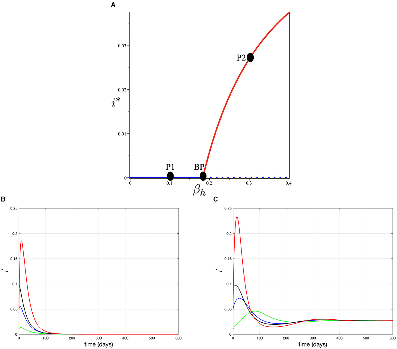
Figure 2. (A) Bifurcation diagram of system (3) in βh − i plane, (B) trajectory of solution at point P1 (when βh = 0.1) for various initial condition tends to monkeypox free equilibrium, and (C) trajectory of solution at point P2 (when βh = 0.3) for various initial condition tends to monkeypox endemic equilibrium.
4 Optimal control problem
4.1 Optimal control model
Here, in this section, we extend our model in Equation (1) by implementing three different control variables, namely the self-protection (u1(t)), hospitalization (u2(t)), and disinfectant to reduce virus in the surface (u3(t)).
1. Self-protection (u1(t)). To reduce human-to-human contact and prevent the spread of monkeypox (monkeypox), several measures can be taken. These include social distancing, practicing good hygiene, and wearing a face mask [27, 37, 38]. We assume that u1(t) is the proportion of humans who are using self-protection. We assume that the government consistently promotes a self-awareness campaign to encourage adherence to self-protection measures within the general population. Hence, we define u1(t)N as the proportion of people using self-protection at time t. There are three possible incidences of contact based on the use of self-protection. First, when both individuals employ self-protection, it is indicated by . Second, when only one uses self-protection, then it is indicated by u1N(1 − u1)N. The last is when both the individuals do not use self-protection, which is indicated by contact between (1 − u1)N and (1 − u1)N. Let us assume that this self-protection will reduce the chance of transmission rate β by a factor ξ1 if people who made contact both using self-protection, ξ2 if only one of them uses self-protection, and no reduction if no one uses self-protection. Hence, the total of new infections of monkeypox when there is a proportion of u1 who use self-protection is given by
For the sake of simplification, we denote
2. Hospitalization (u2(t)). Individuals admitted to the hospital due to monkeypox are typically provided with supportive measures, including pain relief, antiviral medications, fluid replacement, and interventions to address potential complications such as pneumonia or sepsis. While no specific treatments exclusively target monkeypox, certain antiviral medications, such as tecovirimat (TPOXX), brincidofovir, and cidofovir, can be employed to aid in managing the infection [39–41]. We assume only a proportion of monkeypox-infected individuals get hospitalized, with a proportion of u2. These hospitalized individuals will get proper treatment which will increase their recovery rate from γ0 to γ1. Hence, the total of recovered infected individuals is given by
For the sake of simplification, let k2(u2(t))= (γ1u2(t)+ (1 − u2(t)) γ0).
3. Disinfectant (u3(t)). Regularly disinfecting contaminated surfaces is crucial in controlling the spread of monkeypox, as it reduces the viability and transmission of the virus from surfaces to humans. The lessons we have learned from the COVID-19 pandemic highlight the significance of frequent surface disinfection to prevent the spread of viruses. Effective disinfectants, including those proven effective against SARS-CoV-2, can also be beneficial in combating monkeypox. By implementing rigorous disinfection protocols, especially for frequently touched surfaces and in healthcare settings, we can minimize the risk of surface-mediated transmission of the disease [42, 43]. We assume that the use of disinfectant will kill the free viruses on the environment's surface. We assume this disinfectant is implemented with a rate of u3(t). Hence, with this intervention, the C compartment will reduce not only by μp but also by u3(t).
With the above explanation, the model in Equation (1) now reads as follows.
where and k2(u2(t)) = (γ1u2(t) + (1 − u2(t))γ0).
Assuming , , βp = βcN and r = 1 − s − e − i, then we have system (Equation 6) reduced as follows.
Our aim is to reduce the proportion of infected individuals e and i and also contaminated surfaces with a minimum cost for intervention ui(t) for i = 1, 2, 3 which represent self-protection, hospitalization, and disinfectant, respectively. Mathematically, it can be done by minimizing the following cost function
where ωi > 0 for i = 1, 2, 3 represent the weight parameter for e, i, and c, respectively. On the other hand, ϕi > 0 for i = 1, 2, 3 represent the weight cost for control variable u1(t), u2(t), and u3(t), respectively.
If we assume that u1(t) = u1, u2(t) = u2, u2(t) = u2, k1(u1(t)) = k1, and k2(u2(t)) = k2, then the control reproduction number of system (Equation 7) can be expressed as
From the provided expression, it is apparent that c(u1 = 0, u2 = 0, u3 = 0) = 0.
4.2 Existence of solution
Theorem 9. There exists an optimal control function as well as its corresponding set of solution s*(t), e*(t), i*(t), c*(t), thereby
Proof. In this proof, we follow the process in Xu et al. [44]. The theorem's proof can be demonstrated using the Cesari Theorem [45], which fulfills the following conditions:
1. The set of controls and state variables is non-empty.
2. The set of controls is both closed and convex.
3. The right-hand side of system (Equation 7) is limited by a linear function of the state and control variables.
4. The integrand within the objective function exhibits convexity concerning the input controls .
5. There is a constant C1 > 1, along with positive numbers C2 and C3, such that:
Clearly, when the system exhibits uniform Lipschitz continuity, both set U and the set of solutions for initial values are not empty [46], thereby fulfilling condition 1. Condition 2 and condition 4 are confirmed based on the given definition. Condition 3 can be shown to be true by following the discussion below. This argument is similar to classical arguments that have been presented in Fister et al. [47].
The system (Equation 7) can be expressed as:
where x(t) = [s(t) e(t) i(t) c(t)]T represents the vector of state variables, while matrix A and the non-linear function F(x) are defined as follows:
As a result of applying the Hölder inequality, F(x) fulfills the following condition:
implies
where Q = max{P, ‖A‖} < ∞.
Hence, the function G(x) exhibits uniform Lipschitz continuity, fulfilling the assumption of condition 1, and meets the prescribed bound (Equation 10) specified in the Cesari Theorem. The control signals are confined within the closed set , and the objective function's value in (Equation 8) is bounded in the compact interval [0, 1]. Consequently, the function G(x) is linear in ui, i = 1, 2, 3. This satisfies condition 3.
The objective function (Equation 8) meets the condition (Equation 9), by selecting , and C3 = Δ(0). Thus, condition 5 is established.
4.3 Optimal control characterization
The application of Pontryagin's minimum principle [48] leads us to define the Hamiltonian function as
where the costate variable λi and its coefficients correspond to the right-hand side of the model for the ith state variable.
The adjoint system can be obtained by calculating the partial derivatives of with respect to each of the state variables, resulting in the following:
with the transversality conditions λi(tf) = 0, i = 1, 2, 3.
We can determine the optimal solution for u1, u2, and u3 by utilizing the relevant conditions derived from Pontryagin's principle. This involves differentiating with respect to each control variable and subsequently solving the resulting equations to obtain the expression for the control variables u1, u2, and u3 as follows:
Thus, the optimal control solution can be precisely characterized by the given formula:
5 Numerical experiments
5.1 Sensitivity of the control reproduction number
An elasticity sensitivity analysis is conducted to identify the key parameters influencing the transmission and spread of monkeypox. The sensitivity index is used to assess the relative impact of parameters on the basic reproduction number c and aids in designing effective control measures [49]. The parameter values are obtained from Table 1. An index value that is negative (or positive) signifies an inverse (or direct) influence of the respective parameter on c. The sensitivity index of 0 with respect to the parameter θ is expressed as
Consequently,
Upon substituting the parameter values provided in Table 1, u1 = 0.4, u2 = 0.4, u3 = 0.4 for c = 0.6570877605 < 1, and u1 = 0.1, u2 = 0.1, u3 = 0.1 for c = 1.503519079 > 1. In addition, the assumed values for γ1, ξ1, and ξ2 are , 0.5, and 0.3, respectively. The corresponding elasticity sensitivity indices are presented in Table 2. Furthermore, Figure 3 displays a graphical representation in the form of a bar plot. In the scenario where c < 1, signifying the absence of an outbreak in the disease spread, Figure 3A illustrates that the most sensitive parameter influencing c is βh, the transmission rate between humans. This underscores the pivotal role of human-to-human transmission in preventing an outbreak. On the contrary, when c > 1, indicating the presence of an outbreak, Figure 3B reveals that the sensitivity of c is primarily influenced by two key parameters: γ0, the recovery rate of the infected individuals, and βh, the human-to-human transmission rate. This dual sensitivity emphasizes the importance of recovery dynamics and the rate of transmission between humans in understanding and mitigating the outbreak dynamics of monkeypox.
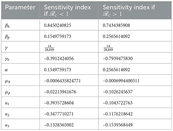
Table 2. Sensitivity index of the parameters in c using parameter values in Table 1, except u1, u2, and u3.
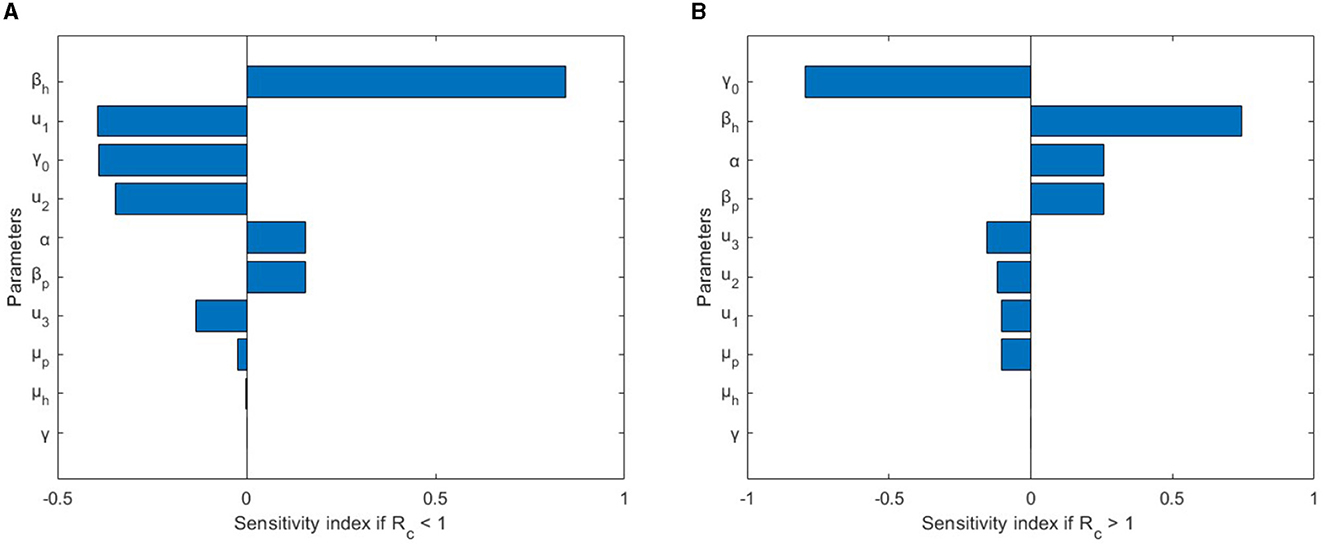
Figure 3. Sensitivity analysis of c. (A) c < 1. (B) c > 1.
We conclude this sensitivity analysis section by presenting a two-parameter sensitivity analysis regarding the control parameters u1, u2, and u3. The results can be observed in Figure 4. In Figure 4A, we depict how the control reproduction number, c, varies with the self-protection (u1) and hospitalization (u2) control parameters. It is evident that increasing the values of u1 and u2 can significantly decrease the magnitude of c. The sensitivity of both u1 and u2 appears to be equally dominant in reducing c. The same observation holds for Figures 4B, C, where increasing the values of parameters u1, u2, and u3 can reduce the value of c. However, it is evident from this numerical experiment that the parameter u3 is not as significant in suppressing the magnitude of c, as indicated in Figures 4B, C. This finding aligns with the results of the elasticity index analysis shown in Figure 3.
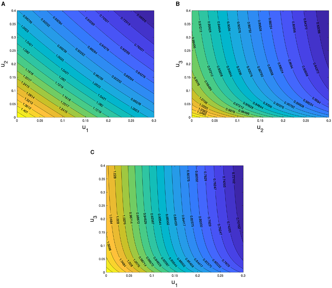
Figure 4. Sensitivity analysis of c with respect to (A) u1 and u2, (B) u2 and u3, and (C) u1 and u3.
5.2 Optimal control simulations
In this section, we investigate the implications of several of optimal control strategies for reducing the prevalence of monkeypox within the human population. Our focus is specifically directed toward assessing the potential of combined control measures to stop the disease's transmission. We aim to provide a demonstrative analysis through numerical simulations of the monkeypox model, both with and without the incorporation of optimized control interventions, to examine the influence of the control variables introduced in the preceding section.
Investigations are conducted into the effects of various combinations of optimal control strategies represented by u1, u2, and u3. These strategies are systematically categorized into three distinct scenarios: single control, double controls, and triple controls, facilitating a coherent grouping of the seven potential control strategies that have been simulated in this study. To clarify, these strategies are defined as follows: Strategy 1 uses only u1, Strategy 2 uses only u2, Strategy 3 uses only u3, Strategy 4 uses both u1 and u2, Strategy 5 uses both of u1 and u3, Strategy 6 uses both of u2 and u3, and Strategy 7 uses of all three controls u1, u2, and u3.
In the following, a comprehensive simulation along with an analysis and discussion of these seven interventions are presented.
1. Single intervention
The influence of employing Strategy 1 (self-protection control, u1 only) on the transmission of monkeypox within the population is illustrated in Figure 5. The implementation of this optimal control results in a 58.7% reduction of the infected human population, as evident in Figure 5C after 50 days. Conversely, the susceptible population exhibits a 46.2% increase, as depicted in Figure 5A. The control profiles that correspond to Strategy 1 are illustrated in Figure 5E. The self-protection control profile shows a constant level of 79% until day 45, at which point it gradually declines monotonically until it reaches its lowest threshold. This pattern suggests an early phase marked by a strong self-defense mechanism deployment, which may be suggestive of a critical phase during the management of the disease. Over time, there is a deliberate decrease in the intensity of these measures.
Figure 7 (as in Appendix A) illustrates the impact of implementing Strategy 2 (use of hospitalization intervention, u2 only) on the dissemination and transmission of monkeypox. The susceptible population experiences a rapid increase with the application of control compared to the scenario without control, as depicted in Appendix Figure 7A, with a 34.6% rise observed after 50 days. When the strategy is used to its fullest potential, as illustrated in Appendix Figure 7C, there is a notable reduction in the population of infected humans, amounting to 51.6%. Appendix Figure 7E analyzes the control profiles of each control variable in strategy 2. The control profile for hospitalization reveals a distinctive curve, commencing at 60%, gradually decreasing until day 10. Following this decline, the curve maintains near-constant levels at 30% until day 30, indicating a stable phase in hospitalization measures. Subsequently, there is a further monotonic decrease reaching zero, indicating a strategic reduction in hospitalization efforts after an initial period of intensity.
Figure 8 (as in Appendix A) displays time series plots showing the effect of applying Strategy 3 (disinfectant control, u3 alone). Using a singular application of disinfectant control results in reduced exposure of susceptible individuals by 48.9% at day 50, as illustrated in Appendix Figure 8B. Consequently, this leads to a decline in the overall number of infected individuals within the population, as demonstrated in Appendix Figure 8C, with a reduction of 46.9%. It is noted that the decrease in contaminated surfaces concentration occurs more rapidly compared to preceding strategies, as represented in Appendix Figure 8D. Following Appendix Figure 8E, we present the control profiles associated with this strategy. A distinct pattern can be seen in the control profile for disinfectant application on contaminated surfaces, which first increases in a curve before peaking at 90%. The curve then starts to progressively decline until it reaches its lowest value. This profile proposes a strategic and efficient use of disinfectant, stressing a thorough application at first and a gradual, deliberate reduction in intensity over time.
2. Combination of two interventions
The impact of employing Strategy 4 (combination of self-protection and hospitalization controls) on the dynamics of monkeypox within the population is depicted in Appendix Figure 9. A greater number of susceptible individuals are shielded during the intervention period, and the size of the infected population notably decreased after a few days of employing this strategy, as shown in Appendix Figures 9A, C, respectively. Specifically, there is a 59.6% increase in susceptible individuals and a remarkable 79% decrease in the infected population.
As in Appendix A, Figure 10, we showcase the simulation of Strategy 5 involving the combination of the use of self-protection and disinfectant controls on the population. There is a remarkable reduction in both the infected human population and contaminated surfaces when the combined interventions are applied, in comparison to the scenario without control, as illustrated in Appendix Figures 10B, D. This results in an 85.5% reduction in the infected population and a significant 93.1% reduction in contaminated surfaces.
Figure 11 (see Appendix A) displays the influence of Strategy 6, optimizing the use of hospitalization and disinfectant controls on the dynamics of monkeypox transmission. The impact of the combined interventions on contaminated surfaces mirrors the findings in Strategy 5 (see Appendix Figures 10D, 11D). It is noteworthy, though, that in this particular intervention, the reduction in the number of infected individuals occurs more rapidly, as Appendix Figure 11C illustrates.
3. Combination of three interventions
The effect of Strategy 7 (combination of self-protection, hospitalization, and disinfectant) on the dynamic behavior of monkeypox is presented in Figure 12 in Appendix A, where Appendix Figure 12E specifically shows the plots displaying the control profiles for all optimal control variables in this strategy. It is observed that the susceptible and exposed individuals, in addition to contaminated surfaces, are in the best results in all strategies as revealed in Appendix Figures 12A, B, D. On the contrary, this is not the case for the number of infected individuals (see Appendix Figure 12C).
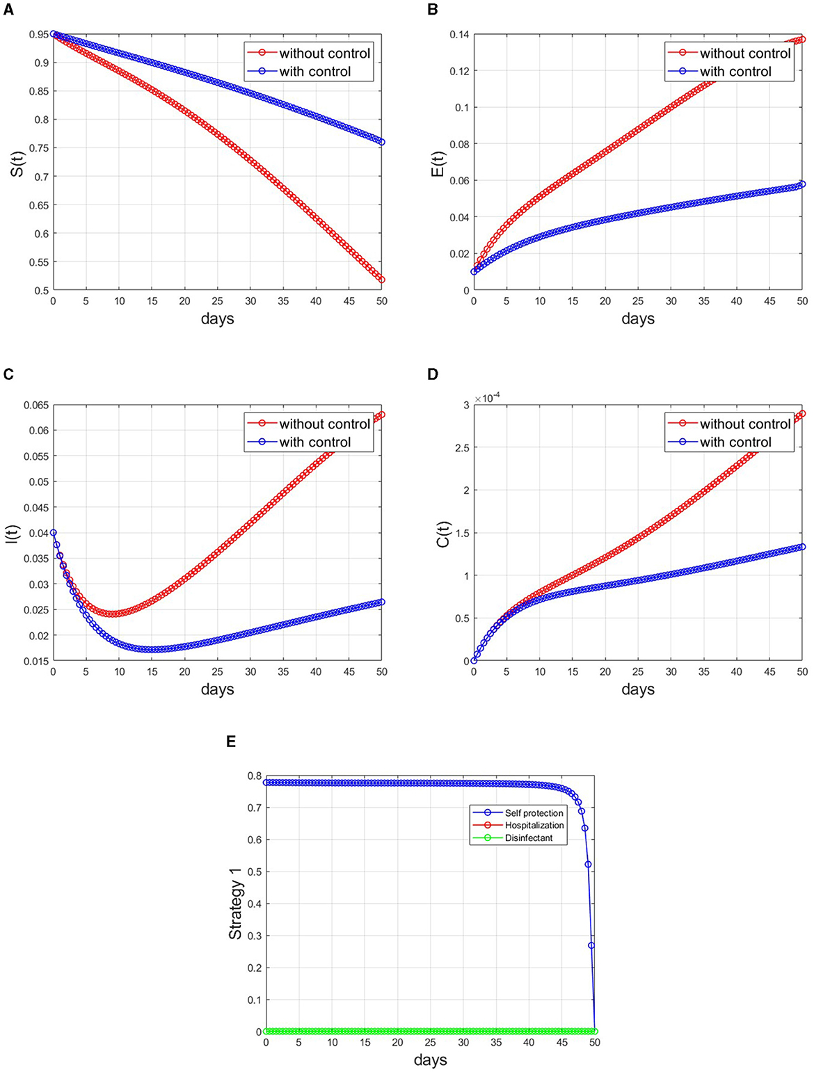
Figure 5. Simulations applying Strategy 1 to the optimal control model. (A) Susceptible individuals, (B) exposed individuals, (C) infected individuals, (D) contaminated surfaces, and (E) control profile.
5.3 Cost-effectiveness analysis
The objective here is to evaluate the most cost-effective strategy among the mentioned monkeypox control techniques in a setting with limited resources. To achieve this, we employ metrics such as the Infection Averted Ratio (IAR) and Average Cost-Effectiveness Ratio (ACER) [50]. Applying the mathematical definitions of these economic assessments as outlined in Asamoah et al. [50], the outcomes of these calculations are presented in Table 3.
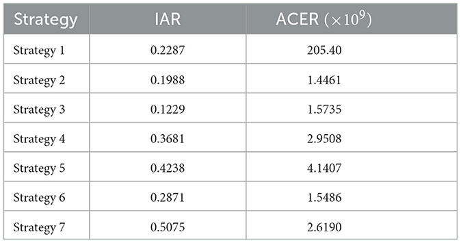
Table 3. IAR and ACER for all strategies.
When employing the Infection Averted Ratio, the strategy exhibiting the largest IAR value is considered the most effective one [51]. Figure 6A suggests that the strategy yielding the highest cost-effectiveness is Strategy 7, which involves the combined use of self-protection, hospitalization, and disinfectant.
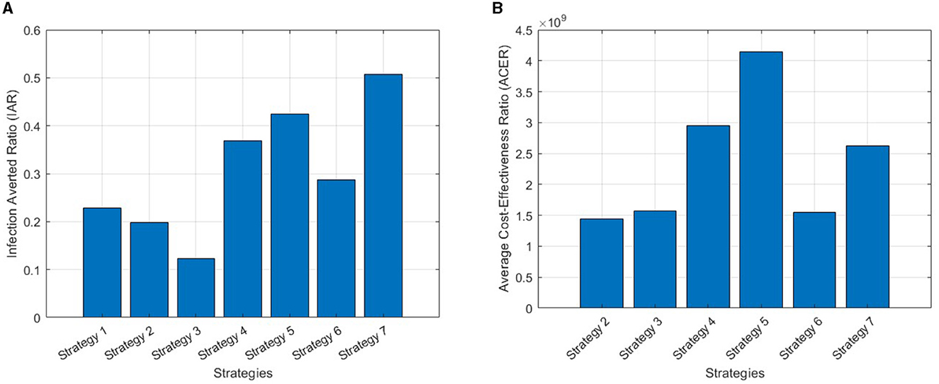
Figure 6. (A) IAR plots for all strategies. (B) ACER plots for all strategies except Strategy 1, as its value exceeds the range of the figure's index.
On the other hand, the strategy exhibiting the lowest ACER ratio is deemed the most cost-effective, in accordance with the Average Cost-Effectiveness Ratio methodology [51]. Strategy 2, as can be seen in Figure 6B, emerges as the most cost-effective strategy, involving the use of hospitalization only.
6 Conclusion
A mathematical model for monkeypox transmission considering contaminated surfaces in the transmission process is considered in this article. The model was developed based on an SEIRC model. Given the comprehensive analysis presented in this study on the transmission dynamics of monkeypox, incorporating contaminated surfaces into a deterministic mathematical model, several key findings emerge. The calculated basic reproduction number serves as a critical threshold, with a forward bifurcation occurring when it equals unity, signifying a pivotal point for disease spread. The absence of a backward bifurcation underscores the singular significance of the basic reproduction number as the sole indicator of the model's endemicity.
The stability analysis, focusing on disease-free and endemic equilibria, establishes global stability conditions based on the basic reproduction number. Notably, the study emphasizes the global stability of the monkeypox-free equilibrium when the reproduction number is below one, contrasting with the instability observed when it exceeds this threshold. The existence and global stability of the endemic equilibrium become evident when the reproduction number surpasses one.
To deepen insights into control strategies, sensitivity analysis identifies influential parameters. This leads to the formulation of an optimal control problem, encompassing self-protection, hospitalization, and disinfection as key interventions. Existence of the solution of the optimal control problem is shown analytically. The Pontryagin Maximum Principle is used to characterize the optimal control problem, giving us the set of adjoint equations and showing optimality conditions.
Numerical simulations explore various control scenarios, demonstrating the efficacy of implemented measures in curbing monkeypox spread. Cost-effectiveness analyses, employing IAR and ACER criteria, underscore the superiority of combined interventions, particularly the synergistic effect of self-protection and disinfection. The IAR results indicate that Strategy 7 is the optimal approach, whereas the ACER metric favors Strategy 2.
The findings of this research underscore the critical role of contaminated surfaces in disease transmission, advocating for targeted control measures. These results align with the conclusions reached by previous studies [5, 23], further supporting the existing body of research highlighting the significant contribution of surface contamination to the spread of infectious diseases. The suggested optimal control strategies, validated through rigorous analysis and simulations, provide valuable insights for evidence-based approaches in mitigating the impact of monkeypox. Additionally, future research considerations, such as incorporating human awareness and assessing the impact of animals as potential vectors, offer avenues for further improvement and a more comprehensive understanding of the dynamics involved in combatting the spread of monkeypox.
Data availability statement
The original contributions presented in the study are included in the article/Supplementary material, further inquiries can be directed to the corresponding author.
Author contributions
AH: Data curation, Formal analysis, Investigation, Methodology, Software, Visualization, Writing – original draft, Writing – review & editing. DA: Conceptualization, Funding acquisition, Investigation, Methodology, Project administration, Supervision, Writing – original draft, Writing – review & editing. MN: Data curation, Investigation, Methodology, Resources, Supervision, Validation, Visualization, Writing – review & editing.
Funding
The author(s) declare financial support was received for the research, authorship, and/or publication of this article. This research was funded by the Ministry of Research, Technology and Higher Education Indonesia (ID number: NKB-1132/UN2.RST/HKP.05.00/2023).
Acknowledgments
The authors thank all reviewers for their constructive suggestions.
Conflict of interest
The authors declare that the research was conducted in the absence of any commercial or financial relationships that could be construed as a potential conflict of interest.
Publisher's note
All claims expressed in this article are solely those of the authors and do not necessarily represent those of their affiliated organizations, or those of the publisher, the editors and the reviewers. Any product that may be evaluated in this article, or claim that may be made by its manufacturer, is not guaranteed or endorsed by the publisher.
Supplementary material
The Supplementary Material for this article can be found online at: https://www.frontiersin.org/articles/10.3389/fams.2024.1372579/full#supplementary-material
References
1. WHO Recommends New Name for Monkeypox Disease. Available online at: https://www.who.int/news/item/28-11-2022-who-recommends-new-name-for-monkeypox-disease (accessed July 7, 2023).
2. Gessain A, Nakoune E, Yazdanpanah Y. Monkeypox. N Engl J Med. (2022) 387:1783–93. doi: 10.1056/NEJMra2208860
3. Beeson A, Styczynski A, Hutson CL, Whitehill F, Angelo KM, Minhaj FS, et al. Mpox respiratory transmission: the state of the evidence. Lancet Microbe. (2023) 4:e277–83. doi: 10.1016/S2666-5247(23)00034-4
4. Boone SA, Gerba CP. Significance of fomites in the spread of respiratory and enteric viral disease. Appl Environ Microbiol. (2007) 73:1687. doi: 10.1128/AEM.02051-06
5. Addai E, Ngungu M, Omoloye MA, Marinda E. Modelling the impact of vaccination and environmental transmission on the dynamics of monkeypox virus under Caputo operator. Math. Biosci. Eng. (2023) 20:10174–99. doi: 10.3934/mbe.2023446
6. Wilson ME, Hughes JM, McCollum AM, Damon IK. Human monkeypox. Clin Infect Dis. (2014) 58:260–7. doi: 10.1093/cid/cit703
7. Mpox Outbreak Global Map | Mpox | Poxvirus | CDC. Available online at: https://www.cdc.gov/poxvirus/mpox/response/2022/world-map.html (accessed July 7, 2023)
8. Nuzzo JB, Borio LL, Gostin LO. The WHO declaration of monkeypox as a global public health emergency. JAMA. (2022) 328:615–7. doi: 10.1001/jama.2022.12513
9. Lai CC, Hsu CK, Yen MY, Lee PI, Ko WC, Hsueh PR. Monkeypox: an emerging global threat during the COVID-19 pandemic. J. Microbiol. Immunol. Infect. (2022) 55:787–94. doi: 10.1016/j.jmii.2022.07.004
10. Lahariya C, Thakur A, Dudeja N. Monkeypox disease outbreak (2022): epidemiology, challenges, and the way forward. Indian Pediatr. (2022) 59:636–42. doi: 10.1007/s13312-022-2578-2
11. Okonji OC, Okonji EF. Monkeypox during COVID-19 era in Africa: current challenges and recommendations. Ann Med Surg. (2022) 81:104381. doi: 10.1016/j.amsu.2022.104381
12. Kraemer MUG, Tegally H, Pigott DM, Dasgupta A, Sheldon J, Wilkinson E, et al. Tracking the 2022 monkeypox outbreak with epidemiological data in real-time. Lancet Infect Dis. (2022) 22:941–2. doi: 10.1016/S1473-3099(22)00359-0
14. Quarleri J, Delpino MV, Galvan V. Monkeypox: considerations for the understanding and containment of the current outbreak in non-endemic countries. GeroScience. (2022) 44:2095–103. doi: 10.1007/s11357-022-00611-6
15. Reynolds MG, Carroll DS, Karem KL. Factors affecting the likelihood of monkeypox's emergence and spread in the post-smallpox era. Curr Opin Virol. (2012) 2:335–43. doi: 10.1016/j.coviro.2012.02.004
16. Mahase E. Monkeypox: what do we know about the outbreaks in Europe and North America? BMJ. (2022) 377:o1274. doi: 10.1136/bmj.o1274
17. Al-Shomrani MM, Musa SS, Yusuf A. Unfolding the transmission dynamics of monkeypox virus: an epidemiological modelling analysis. Mathematics. (2023) 11:1121. doi: 10.3390/math11051121
18. Okyere S, Ackora-Prah J. Modeling and analysis of monkeypox disease using fractional derivatives. Results Eng. (2023) 17:100786. doi: 10.1016/j.rineng.2022.100786
19. Peter OJ, Kumar S, Kumari N, Oguntolu FA, Oshinubi K, Musa R. Transmission dynamics of Monkeypox virus: a mathematical modelling approach. Model Earth Syst Environ. (2022) 8:3423–34. doi: 10.1007/s40808-021-01313-2
20. Alharbi R, Jan R, Alyobi S, Altayeb Y, Khan Z. Mathematical modeling and stability analysis of the dynamics of monkeypox via fractional-calculus. Fractals. (2022) 30:2240266. doi: 10.1142/S0218348X22402666
21. Michael UE, Omenyi LO, Kafayat E, Nwaeze E, Akachukwu OA, Ozoigbo G, et al. Monkeypox mathematical model with surveillance as control. Commun Math Biol Neurosci. (2023) 2023:6. doi: 10.28919/cmbn/7781
22. El-Mesady A, Elsonbaty A, Adel W. On nonlinear dynamics of a fractional order monkeypox virus model. Chaos Solitons Fractals. (2022) 164:112716. doi: 10.1016/j.chaos.2022.112716
23. Alshehri A, Ullah S. Optimal control analysis of Monkeypox disease with the impact of environmental transmission. AIMS Math. (2023) 8:16926–60. doi: 10.3934/math.2023865
24. Alzubaidi AM, Othman HA, Ullah S, Ahmad N, Alam MM. Analysis of Monkeypox viral infection with human to animal transmission via a fractional and Fractal-fractional operators with power law kernel. Math Biosci Eng. (2023) 20:6666–90. doi: 10.3934/mbe.2023287
25. Li C, Samreen, Ullah S, Nawaz R, AlQahtani SA, Li S. Mathematical modeling and analysis of monkeypox 2022 outbreak with the environment effects using a Cpauto fractional derivative. Phys Scr. (2023) 98:105239. doi: 10.1088/1402-4896/acf88e
26. Madubueze CE, Onwubuya IO, Nkem GN, Chazuka Z. The transmission dynamics of the monkeypox virus in the presence of environmental transmission. Front Appl Math Stat. (2022) 8:1061546. doi: 10.3389/fams.2022.1061546
27. Mpox (monkeypox). Available online at: https://www.who.int/news-room/fact-sheets/detail/monkeypox (accessed July 23, 2023).
28. Morgan CN, Whitehill F, Doty JB, Schulte J, Matheny A, Stringer J, et al. Environmental persistence of monkeypox virus on surfaces in household of person with travel-associated infection, Dallas, Texas, USA, 2021. Emerg Infect Dis. (2022) 28:1982. doi: 10.3201/eid2810.221047
29. Brauer F, Castillo-Chavez C, Feng Z. Endemic disease models. Math Models Epidemiol. (2019) 69:63. doi: 10.1007/978-1-4939-9828-9_3
30. Aldila D, Ndii MZ, Anggriani N, Windarto, Tasman H, Handari BD. Impact of social awareness, case detection, and hospital capacity on dengue eradication in Jakarta: a mathematical model approach. Alex Eng J. (2023) 64:691–707. doi: 10.1016/j.aej.2022.11.032
31. Diekmann O, Heesterbeek JAP, Roberts MG. The construction of next-generation matrices for compartmental epidemic models. J R Soc Interface. (2010) 7:873–85. doi: 10.1098/rsif.2009.0386
32. Driessche PVD, Watmough J. Reproduction numbers and sub-threshold endemic equilibria for compartmental models of disease transmission. Math Biosci. (2002) 180:29–48. doi: 10.1016/S0025-5564(02)00108-6
33. Bavafa-Toosi Y. Stability analysis. Introduction Linear Control Syst. (2019) 2019:265–31. doi: 10.1016/B978-0-12-812748-3.00003-3
34. Alqahtani H, Badshah Q, Sakhi S, ur Rahman G, Gmez-Aguilar JF. Qualitative aspects and sensitivity analysis of MERS-Corona epidemic model with and without noise. Phys Scr. (2023) 98:125018. doi: 10.1088/1402-4896/ad0bb6
35. Martcheva M. An Introduction to Mathematical Epidemiology, Volume 61. Berlin: Springer US. (2015). doi: 10.1007/978-1-4899-7612-3
36. Castillo-Chavez C, Song B. Dynamical models of tuberculosis and their applications. Math Biosci Eng. (2004) 1:361–404. doi: 10.3934/mbe.2004.1.361
37. How to Protect Yourself | Mpox | Poxvirus | CDC. Available online at: https://www.cdc.gov/poxvirus/mpox/prevention/protect-yourself.html (accessed July 23, 2023).
38. Mpox (monkeypox): How it Spreads, Prevention and Risks - Canada.ca. Available online at: https://www.canada.ca/en/public-health/services/diseases/mpox/risks.htmla3 (accessed July 23, 2023).
39. Miller MJ, Cash-Goldwasser S, Marx GE, Schrodt CA, Kimball A, Padgett K, et al. Severe monkeypox in hospitalized patients — United States, August 10–October 10, 2022. MMWR Morb Mortal Wkly Rep. (2022) 71:1412–7. doi: 10.15585/MMWR.MM7144E1
40. Benites-Zapata VA, Ulloque-Badaracco JR, Alarcon-Braga EA, Hernandez-Bustamante EA, Mosquera-Rojas MD, Bonilla-Aldana DK, et al. Clinical features, hospitalisation and deaths associated with monkeypox: a systematic review and meta-analysis. Ann Clin Microbiol Antimicrob. (2022) 21:1–18. doi: 10.1186/s12941-022-00527-1
41. DeWitt ME, Polk C, Williamson J, Shetty AK, Passaretti CL, McNeil CJ, et al. Global monkeypox case hospitalisation rates: a rapid systematic review and meta-analysis. eClinicalMedicine. (2022) 54:101710. doi: 10.1016/j.eclinm.2022.101710
42. Kampf G, Todt D, Pfaender S, Steinmann E. Persistence of coronaviruses on inanimate surfaces and their inactivation with biocidal agents. J Hosp Infect. (2020) 104:246–51. doi: 10.1016/j.jhin.2020.01.022
43. About List N: Disinfectants for Coronavirus (COVID-19) | US EPA. Available online at: https://www.epa.gov/coronavirus/about-list-n-disinfectants-coronavirus-covid-19-0 (accessed August 5, 2023).
44. Xu D, Xu X, Xie Y, Yang C. Optimal control of an SIVRS epidemic spreading model with virus variation based on complex networks. Commun Nonlinear Sci Numer Simul. (2017) 48:200–10. doi: 10.1016/j.cnsns.2016.12.025
45. Fleming WH, Rishel RW. Deterministic and Stochastic Optimal Control. Google Books. Available online at: https://scholar.google.com/scholar_lookup?title=Deterministic%20and%20stochastic%20optimal%20control&publication_year=1975&author=W.H.%20Fleming&author=R.W.%20Rishel (Accessed August 9, 2023).
46. Birkhoff G, Rota G-C. Ordinary Differential Equation, 4th ed. New York, NY: Wiley (1989). References - Scientific Research Publishing. Available online at: https://www.scirp.org/ (accessed August 9, 2023).
47. Fister KR, Lenhart S, McNally JS. Optimizing chemotherapy in an HIV model. Electron J Differ Equ. (1998) 1998:1–12.
48. Pontryagin LS. Mathematical Theory of Optimal Processes. London: Routledge (2018) doi: 10.1201/9780203749319
49. Wu J, Dhingra R, Gambhir M, Remais JV. Sensitivity analysis of infectious disease models: methods, advances and their application. J R Soc Interface. (2013) 10:20121018. doi: 10.1098/rsif.2012.1018
50. Asamoah JKK, Yankson E, Okyere E, Sun GQ, Jin Z, Jan R, et al. Optimal control and cost-effectiveness analysis for dengue fever model with asymptomatic and partial immune individuals. Results Phys. (2021) 31:104919. doi: 10.1016/j.rinp.2021.104919
Keywords: monkeypox, mathematical model, stability analysis, optimal control, contaminated surfaces
Citation: Hassan AH, Aldila D and Noor Aziz MH (2024) Optimal control and stability analysis of monkeypox transmission dynamics with the impact of contaminated surfaces. Front. Appl. Math. Stat. 10:1372579. doi: 10.3389/fams.2024.1372579
Received: 18 January 2024; Accepted: 06 February 2024;
Published: 01 March 2024.
Edited by:
Nossaiba Baba, University of Hassan II Casablanca, MoroccoReviewed by:
Asmaa Idmbarek, University of Hassan II Casablanca, MoroccoImane Agmour, University of Hassan II Casablanca, Morocco
Copyright © 2024 Hassan, Aldila and Noor Aziz. This is an open-access article distributed under the terms of the Creative Commons Attribution License (CC BY). The use, distribution or reproduction in other forums is permitted, provided the original author(s) and the copyright owner(s) are credited and that the original publication in this journal is cited, in accordance with accepted academic practice. No use, distribution or reproduction is permitted which does not comply with these terms.
*Correspondence: Dipo Aldila, YWxkaWxhZGlwb0BzY2kudWkuYWMuaWQ=