Variational Bayes latent class analysis for EHR-based phenotyping with large real-world data

Introduction: Bayesian approaches to patient phenotyping in clinical observational studies have been limited by the computational challenges associated with applying the Markov Chain Monte Carlo (MCMC) approach to real-world data. Approximate Bayesian inference via optimization of the variational evidence lower bound, variational Bayes (VB), has been successfully demonstrated for other applications.

Methods: We investigate the performance and characteristics of currently available VB and MCMC software to explore the practicability of available approaches and provide guidance for clinical practitioners. Two case studies are used to fully explore the methods covering a variety of real-world data. First, we use the publicly available Pima Indian diabetes data to comprehensively compare VB implementations of logistic regression. Second, a large real-world data set, Optum™ EHR with approximately one million diabetes patients extended the analysis to large, highly unbalanced data containing discrete and continuous variables. A Bayesian patient phenotyping composite model incorporating latent class analysis (LCA) and regression was implemented with the second case study.

Results: We find that several data characteristics common in clinical data, such as sparsity, significantly affect the posterior accuracy of automatic VB methods compared with conditionally conjugate mean-field methods. We find that for both models, automatic VB approaches require more effort and technical knowledge to set up for accurate posterior estimation and are very sensitive to stopping time compared with closed-form VB methods.

Discussion: Our results indicate that the patient phenotyping composite Bayes model is more easily usable for real-world studies if Monte Carlo is replaced with VB. It can potentially become a uniquely useful tool for decision support, especially for rare diseases where gold-standard biomarker data are sparse but prior knowledge can be used to assist model diagnosis and may suggest when biomarker tests are warranted.

1 Introduction

With the growing acceptance by clinical regulators of using real-world evidence to supplement clinical trials, there is increasing interest in the use of Bayesian analysis for both experimental and observational clinical studies [1]. The identification of specific patient groups sharing similar disease-related phenotypes is core to many clinical studies [2]. Secondary use of electronic health records (EHR) data has long been incorporated in phenotypic studies [3]. Recent studies cover a wide range including health economics models [4], innovative trial designs for rare disease drug design [5], and application of EHR information for antibiotic dose calculations [6]. The most popular approach that has evolved for identification of cohorts belonging to a particular phenotype of interest is an expert-driven rule-based heuristic dependent on data availability for a given phenotypic study, for example, Cuker et. al. [7]. The application of machine learning to patient phenotyping has become an active area of research [8] but such approaches do not consider prior knowledge and hence are limited, particularly where data are sparse, for example, with rare diseases. The patient phenotyping approach presented in this study uses Bayesian statistics to provide a formal mathematical method for combining prior information with current information at a study design stage for identification of phenotypes as a means of selecting a study population. This offers a mathematically principled method for incorporating expert opinion and other prior information that can potentially improve study population precision.

Markov Chain Monte Carlo (MCMC) is considered the gold standard for Bayesian inference because, in theory, it asymptotically converges to the true posterior distribution if run for a sufficient number of iterations thereby reaching a stationary posterior distribution [9]. Its application has been limited by the computational challenges of applying MCMC to large real-world clinical data. In Bayesian analysis, we are usually interested in the posterior distribution p(Z|X) where Z are latent variables {z₁, ..., z_n} and X are observed data {x₁, ..., x_n}. In many real-world models of interest, the denominator of Bayes' theorem, p(X), often referred to as the evidence, and evaluates to ∫p(Z, X)dZ, typically gives rise to analytically or computationally intractable integrals [10]. Approximate Bayesian inference via optimization of the one-sided evidence lower bound is often called Variational Bayes (VB) or Variational Inference (VI). In VB, optimization is used to find an optimum distribution q(Z) from a family of tractable distributions Q such that it is as close to the posterior distribution p(Z|X) as possible. The optimization aims to locate q^*(Z), the distribution that minimizes the Kullback-Leibler (KL) divergence of q(Z) and p(Z|X). This optimization approach is often significantly more computationally efficient than MCMC at the expense of an approximated posterior that cannot be improved with more iterations.

VB has been successfully demonstrated for other patient phenotyping applications. Song et al. applied variational inference with a deep learning natural language processing (NLP) approach to patient phenotyping [11]. Li et al. propose another NLP model, MixEHR, that applies a latent topic model to EHR data [12]. They apply a VB coordinate ascent approach to impute mixed disease memberships and latent disease topics that apply to a given patient EHR cohort. Hughes et al. developed a mean-field VB model for multivariate generalized linear mixed models applied to longitudinal clinical studies [13].

Latent class analysis (LCA) is widely used when we want to identify patient phenotypes or subgroups given multivariate data [14]. A challenge in biomedical LCA is the prevalence of mixed data, where we may have combinations of continuous, nominal, ordinal, and count data, further complicated by missing and inaccurate data across variables. Bayesian approaches to LCA may better account for this data complexity. The Bayesian approach serves as a connection between rule-based phenotypes, which heavily depend on medical expert knowledge and opinion, and data-driven machine learning methods that solely rely on the information within the data being analyzed, without the ability to incorporate relevant prior knowledge [15]. White and Murphy [16] included a variational inference approach to latent class analysis with their BayesLCA R package.

Hubbard et al. [17] proposed a composite LCA/regression model that might be used in a general context for observational studies that use EHR data. They consider the common clinical context where gold-standard phenotype information, such as genetic and laboratory data, is not fully available. A general model of this form has high potential applicability for use in clinical decision support across disease areas and with primary and secondary clinical databases. In this study, we want to evaluate VB for this context and compare with several MCMC implementations to determine which are potentially suitable choices for large real-world biomedical studies of this form. Our primary objective is to determine whether VB can enable wider use of Bayesian approaches in large biomedical studies with acceptable accuracy in a clinical setting.

This study is motivated by a patient phenotyping composite Bayes LCA/regression model of the form proposed by Hubbard et al. [17]. It can potentially become a uniquely useful tool for clinical decision support, especially for rare disease areas where gold-standard biomarker data are sparse, if the computational challenges of MCMC can be ameliorated. In this study, we use the same composite Bayesian LCA/regression model form and motivating example as Hubbard et al., namely pediatric T2DM, to test whether the proposed LCA model translates to a different EHR database with the same target disease under study (Optum™ EHR). Pediatric T2DM is rare, so it naturally gives rise to the data quality issues we would like to explore with our approach. We extend the Hubbard et al. study to incorporate VB to investigate whether a much larger EHR data set is amenable to this form of Bayesian model. Our aim in this study is to investigate whether a VB approach to Bayesian LCA/regression phenotyping scales to real-world large EHR data and delivers a posterior approximation acceptably close to MCMC in a clinical setting. We compare a range of readily available VB software within two case studies comparing how closed-form and black-box VB methods perform with clinical data. The structure of the study is as follows. Section 2 details the VB algorithms and available software compared including comparison with a maximum likelihood estimation (MLE) approach for completeness since the majority of clinical analyses currently employ MLE. Note that the aim of this study is to focus on scalable Bayesian methods so we did not carry out a detailed comparison with either machine learning or frequentist/MLE approaches. This section also describes the data used for each case study and how each serves our primary objective of comparing a wide range of VB algorithms and software with a special focus on generalizable Bayesian models for large real-world data; Section 3 presents the results for both use cases; Section 4 concludes with a summary and discussion of advantages and challenges of using VB for EHR-based patient phenotyping with suggestions for further work. The primary goal is matching the gold-standard MCMC algorithm as closely as possible while enabling timely completion of large-scale clinical observational studies.

2 Materials and methods

Our primary objective is to investigate whether a VB approach to a potentially generalizable composite Bayesian LCA/regression phenotyping model scales to real-world large EHR data and delivers a posterior approximation acceptably close to MCMC in a clinical setting. We find there is a lack of available VB software suitable for our composite Bayesian LCA/regression model. For that reason, we included a simpler case study using a purely logistic regression model with the widely available Pima Indians' diabetes data¹. This enabled us to include conditionally conjugate closed-form methods that are available for VB logistic regression in a wider comparison of VB and MCMC.

MCMC has become the de facto gold-standard method for Bayesian analysis due to its theoretical guarantee that, if iterated to infinity, it will eventually sample from the true posterior distribution given by Bayes' rule [18]. In practice, it is difficult to determine how many iterations are needed before an MCMC sampling chain has converged to stable bounds around the true posterior. We therefore usually run several separate sampling chains for some pre-specified number of iterations, including so-called burn-in initial iterations that we ignore for convergence assessment [19]. Convergence assessment usually includes comparison of diagnostic measures between the separate sampling chains [20]. JAGS is a Metropolis-Hastings sampler that specializes in Gibbs sampling [21]. Gibbs sampling can sample discrete and continuous latent parameters. Stan is a Metropolis-Hastings sampler that uses a different approach, Hamiltonian Monte Carlo, that can be faster to reach convergence but, instead of sampling discrete latent variables, integrates across each class of each discrete latent variable [22]. This is a technique called marginalizing-out or integrating-out the discrete latent variables from the posterior distribution². A benefit of marginalizing-out discrete latent variables is a model specification that allows greater exploration of the tails of the distribution (see footnote 2). However, it requires specific Stan model syntax which complicates translation of JAGS models with discrete parameters.

VB has become popular in cases where MCMC computation is particularly challenging. VB employs optimization of the lower bound on the marginal likelihood to minimize the Kullback-Leibler divergence of a member of some posited family of approximations to the real posterior distribution [23]. This lower bound is often referred to as the Evidence Lower Bound (ELBO) or the Bayes free energy. The Blei et. al. [24] comprehensive review of VB address VB from a statistical viewpoint. Their study covers both the deterministic mean-field approach, coordinate ascent variational inference (CAVI) as well as stochastic mean-field optimization that scales to very large data. They provide outline algorithms for both approaches. Stochastic Variational Inference (SVI) makes use of repeated subsampling of the data points to noisily optimize the ELBO [25].

For the logistic regression case study, we compared JAGS and Stan MCMC with ten VB software packages plus a textbook implementation (Table 1). Five of the software packages use automatic black-box approaches. Automatic approaches focus on optimizing difficult variational objectives where the exponential family property for the proposed variational density may not apply [26]. These methods attempt to generalize non-conjugate inference to apply across many models without specific model derivation of the objective functions, hence the “black-box” label. For example, Automatic Differentiation Variational Inference (ADVI) [26] is a hybrid approach using Monte Carlo estimates of the ELBO gradient written as an expectation that can be repeatedly sampled within a stochastic optimization algorithm. ADVI transforms the support of latent variables to the real coordinate space before computing the ELBO using Monte Carlo integration. It then uses stochastic gradient ascent to maximize the ELBO. All of this is performed automatically, without user input.

Table 1

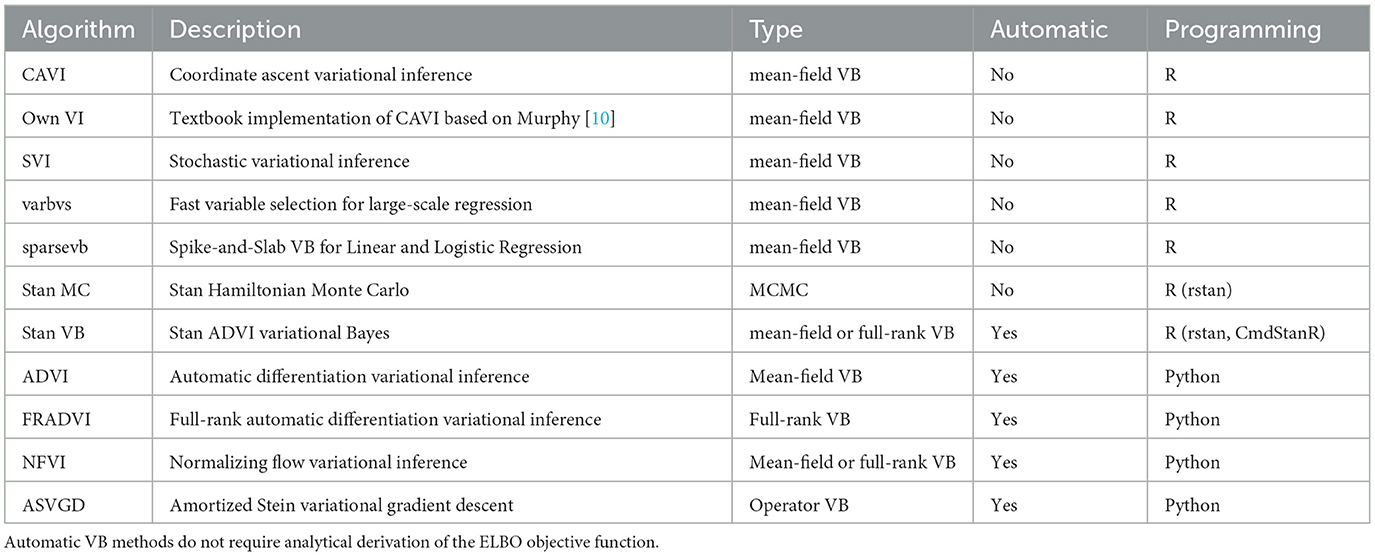
Table 1. VB and MCMC algorithms in the logistic regression case study.

The Stan implementation for ADVI incorporates several algorithm hyperparameters that can be tuned³. We found combinations of several algorithm hyperparameters affected both runtime and how closely the result converged (or failed to converge) to estimates similar to those obtained with MCMC. The iter hyperparameter is important to ensure the algorithm is allowed to run long enough to achieve ELBO convergence. For our EHR data set, we found a large number of iterations were needed (15,000). The default of 10,000 seems a good general starting point. We found the elbo_samples default (100) was far too low for our EHR data. The elbo_samples hyperparameter sets the number of samples for Monte Carlo estimate of the ELBO. For our data, we found best accuracy with a value approximately 10,000. This setting increased the run time of the algorithm to the extent it was not significantly quicker than MCMC. The tol_rel_obj hyperparameter sets the stopping criterion. For our EHR data, we set it lower (0.001) than the default of 0.01 as we found cases where the ELBO had not converged at the time the algorithm stopped. We used the default values for other hyperparameters.

For the Bayesian composite LCA/regression case study, we first reproduced the Hubbard et al. model [17] with JAGS MCMC [21] using the Optum™ EHR T2DM data. This gives us confidence that the composite Bayes LCA/regression model can generalize to other similar EHR data. We then followed up with Stan [22] implementations of Hamiltonian MCMC and VB to investigate how the model specification translates to other algorithmic approaches. As we could not find available closed-form implementations suitable for our composite Bayes LCA/regression model, such as coordinate ascent or stochastic mean-field VB, we used Stan Automatic Differentiation Variational Inference (ADVI) [27] for this case study.

2.1 Logistic regression model

We used the standard logistic regression model for binary classification. Given a data set with n observations and m observed feature variables, where x_i represents the observed variables for the i^th observation, and y_i represents the binary response, the logistic regression model predicts the probability p(y_i = 1|x_i) using the logistic function

$\begin{array}{ll}p(y_i=1|x_i)=\frac{1}{1+e^{-z_i}}& (1)\end{array}$

where z_i is the linear combination of the features and their corresponding coefficients:

$\begin{array}{ll}{z}_i={\beta }_0+{\beta }_1{x}_{i1}+{\beta }_2{x}_{i2}+\cdots +{\beta }_m{x}_{im}& (2)\end{array}$

where β₀ is the intercept coefficient, and we have β_m coefficients for the 1, …, m feature variables. In Bayesian logic regression, we can define priors on the coefficients. We used normal priors in this study as all predictor variables are continuous.

2.1.1 Pima Indians' diabetes data

We used the Kaggle subset¹ of Pima Indian adult T2DM data to facilitate a wide comparison of VB implementations [28]. The response, y_i, is the variable Outcome (diagnosed T2DM). The predictors, x_i, are all continuous variables (pregnancies, glucose, blood pressure, skin thickness, insulin, BMI, diabetes pedigree, and age). A logistic regression model was fitted to all predictors as there are many available VB software implementations for logistic regression so it serves as a suitable comparative baseline approach. Our objective with this case study is to compare conditionally conjugate closed-form methods, for example, [29] with black-box automatic methods, for example, [26] using clinically relevant data.

2.1.2 VB logistic regression software

Two VB software libraries in R were compared; sparsevb [30] and varbvs [31] along with published implementations of CAVI and SVI from the GitHub⁴ of Durante and Rigon [29]. sparsevb uses mean-field CAVI VB. Their package focuses specifically on variable selection in high dimensional data for regression models using a spike-and-slab prior to induce sparsity. Their package includes a novel parameter updating order to improve the CAVI algorithm performance. varbvs is also focused on variable selection, in this case aimed at genome-wide association studies. varbvs is sensitive to the variable ordering and initialization of optimization procedure. The Python library PyMC3 [32] supports four VB methods that were included in this study (Table 1). All four are automatic black-box methods similar to those found in Stan. The ADVI algorithm from PyMC3 has a similar programming approach to Stan. Full-rank ADVI (FRADVI) generalizes the mean-field approximation. The off-diagonal terms in the covariance matrix capture posterior correlations across latent random variables. This should result in a more accurate posterior approximation. The Normalizing Flows VI (NFVI) approach originates from Rezende and Mohamed [33] whereby a standard initial density is transformed into a more complex proposed density by applying a sequence of invertible transformations until a preset level of complexity is obtained. The aim is to improve the posterior accuracy. The Amortized Stein Variational Gradient Descent (ASVGD) approach is from Liu and Stein [34]. ASVGD is related to the study by Rezende and Mohamed [33]. They introduce a particle-based framework that allows for automatic differentiation through stochastic computation graphs to efficiently estimate gradients. In this approach, the mean parameters are treated as a set of particles. We included a naïve textbook implementation of CAVI from Murphy [10] to assess how better the Durante & Rigon published implementation is. We applied 5-fold cross-validation (CV) to the data set to investigate the stability of the different implementations. For algorithms containing hyperparameters, we performed a grid search over a range for each hyperparameter within each CV iteration.

2.2 Composite Bayes LCA/regression model

The canonical form for LCA assumes that each observation i, with U observed categorical response variables x_i = {x_i1, x_i2, …, x_iU}, belongs to one of C latent classes. Class membership is represented by a latent class indicator z_i = {1, ..., C}. The marginal response probabilities are

$\begin{array}{ll}P({\text{x}}_i)={\displaystyle \sum _{c=1}^C}{\pi }_c{\displaystyle \prod _{u=1}^U}P(x_{iu}|z_i=c)& (3)\end{array}$

where z_i is the latent class that observation i belongs to, and π_c is the probability of being in class c. The variables x are assumed to be conditionally independent given class membership, an assumption known as local independence.

The composite Bayes LCA/regression model applied is from Hubbard et al. [17] and follows the general specification shown in Table 2. In the T2DM model example, D_i represents the latent dichotomous propensity for observation i to be in the T2DM class, that is, the value of C in Equation 3 denotes that either the patient has T2DM or does not have T2DM. There are three variables in U; biomarker indicator R_ij, where j has two categories, laboratory test availability for HbA1c and Random Blood Glucose for observation i; ICD clinical codes W_ik, where k has two categories, diagnosis of T2DM and at least one endocrinologist visit; and diabetes medications P_il, where l has two categories, metformin and insulin. The latent phenotype variable for each patient, D_i, is assumed to be associated with patient characteristics that include demographics (for pediatric T2DM, they are age, higher-risk ethnicity, and BMI z-score) denoted by X in the model specification. This model allows for any number of clinical codes or medications, and in this model, each clinical code and medication are binary indicator variables to specify if the code or medication was present for that patient. Since it is common for biomarker laboratory tests, Y_ij, to be missing across a cohort of patients, biomarker availability, R_ij, is an important component of the model. This is because biomarkers are widely considered to be high-quality prognostic data for many disease areas [35] and availability of a biomarker measurement can be predictive of the phenotype since laboratory tests are often proxies for physician diagnoses.

Table 2

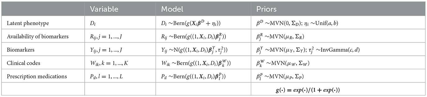
Table 2. Model specification for Bayesian latent variable model for EHR-derived phenotypes for patient i.

The model likelihood for the i^th patient is given by

$\begin{array}{l}L({\eta }_i,{\beta }^D,{\beta }^R,{\beta }^Y,{\beta }^W,{\beta }^P,{\tau }^2|X_i)={\displaystyle \sum _{d=0,1}}P(D_i=d|{\eta }_i,{\beta }^D,X_i)\\ \hspace{1em}\hspace{1em}\hspace{1em}\hspace{1em}\hspace{1em}\hspace{1em}\hspace{1em}\hspace{1em}\hspace{1em}\hspace{1em}\hspace{1em}\hspace{1em}\hspace{1em}{\displaystyle \prod _{j=1}^J}f(R_{ij}|D_i=d,X_i,{\beta }_j^R)f(Y_{ij}|D_i\\ \hspace{1em}\hspace{1em}\hspace{1em}\hspace{1em}\hspace{1em}\hspace{1em}\hspace{1em}\hspace{1em}\hspace{1em}\hspace{1em}\hspace{1em}\hspace{1em}\hspace{1em}=d,X_i,{\beta }_j^Y,{\tau }_j^2{)}^{R_{ij}}\\ \hspace{1em}\hspace{1em}\hspace{1em}\hspace{1em}\hspace{1em}\hspace{1em}\hspace{1em}\hspace{1em}\hspace{1em}\hspace{1em}\hspace{1em}\hspace{1em}\hspace{1em}{\displaystyle \prod _{k=1}^K}f(W_{ik}|D_i=d,X_i,{\beta }_k^W)\\ \hspace{1em}\hspace{1em}\hspace{1em}\hspace{1em}\hspace{1em}\hspace{1em}\hspace{1em}\hspace{1em}\hspace{1em}\hspace{1em}\hspace{1em}\hspace{1em}\hspace{1em}{\displaystyle \prod _{l=1}^L}f(P_{il}|D_i=d,X_i,{\beta }_i^P)& (4)\end{array}$

where β^D associates the latent phenotype to patient characteristics, η_i is a patient-specific random effect parameter, and parameters β^R, β^Y, β^W, and β^P associate the latent phenotype and patient characteristics to biomarker availability, biomarker values, clinical codes, and medications, respectively. X_i represents M patient covariates, such as demographics (X_i = X_i1, ..., X_iM). The mean biomarker values are shifted by a regression quantity ${\beta }_{j,M+1}^Y$ for patients with the phenotype compared to those without⁵. The sensitivity and specificity of binary indicators for clinical codes, medications, and the presence of biomarkers are given by combinations of regression parameters. For instance, in a model with no patient covariates, sensitivity of the k^th clinical code is given by $expit({\beta }_{k_0}^W+{\beta }_{k_1}^W)$, while specificity is given by $1-expit({\beta }_{k_0}^W)$, where expit(·) = exp(·)/(1+exp(·)). We validate this model with a real-world example, namely, pediatric T2DM. Table 3 indicates how the composite Bayes LCA/regression phenotyping model maps to this disease area. f(·) in Equation 4 represents the probability function that will depend on the specific disease application of the model.

Table 3

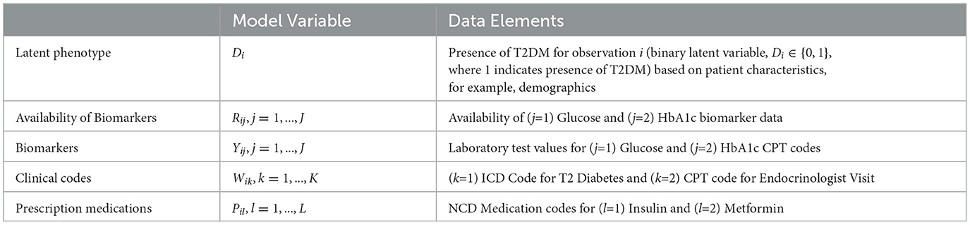
Table 3. Mapping the composite Bayes LCA/regression phenotyping model factors to the pediatric T2DM study for patient i.

Informative priors are used to encode known information on the predictive accuracy of glucose; $Y_{i1}=N(90.6+42D_i,16.93)$ and HbA1c; $Y_{i2}=N(5.4+1D_i,0.45)$ laboratory tests for T2DM. The biomarker priors inform a receiver operating characteristic (ROC) model since the biomarkers are normally distributed. The prior values were selected to correspond to an area under the ROC curve (AUC) of 0.95 [17].

Although the pediatric T2DM example comprises two measured variables for each of Y_i, W_i, and R_i, the model can be expanded to multiple biomarkers, clinical codes, and medications for other disease areas and easily extends to include additional elements, for example, the number of hospital visits or the number of medication prescriptions, or, for other disease conditions or study outcomes, comorbidities, and medical costs. Given our objective is to determine the utility and performance of VB in tackling a problem of this nature, in comparison with MCMC, we extend the Hubbard et al. study by comparing a range of alternative methods to JAGS that included alternative MCMC and VB using Stan. Our aims were to characterize the advantages and challenges posed by this extendable patient phenotyping composite Bayes LCA/regression model using VB approaches compared to the traditional Gibbs/Metropolis-Hastings sampling MCMC approach. The following sub-sections discuss each of these approaches in turn.

2.2.1 Optum™ EHR data

We used licensed Optum™ EHR data for the generalizable Bayesian LCA model. This data set is comprised of EHR records from hospitals, hospital networks, general practice offices, and specialist clinical providers across the United States of America. It includes anonymized patient demographics, hospitalizations, laboratory tests and results, in-patient and prescribed medications, procedures, observations, and diagnoses. The data provide most information collected during a patient journey provided all care sites for a given patient are included in the list of Optum™ data contributors. This data set is one of the most comprehensive EHR databases in the world [36] and is used extensively for real-world clinical studies [37]. The data set used in our case study contains Optum™ EHR records collected between January 2010 and January 2020.

The initial processing step is to identify, from the overall Optum™ data set, a cohort of pediatric patients with elevated risk of T2DM, to subsequently perform phenotyping. For this analysis, we extracted a patient cohort of pediatric patients with equivalent T2DM risk characteristics defined in Hubbard et al. [17]. We transformed our Optum™ data schema into the same form as the Hubbard et al. data schema to test how well the proposed Bayesian LCA model translates from the Hubbard et al. PEDSnet EHR data to the Optum™ EHR data. The PEDSnet data used by Hubbard et al. are located within the USA Northeast region which comprises approximately 13% of the Optum™ data which cover the whole USA. To account for potential variance of pediatric T2DM prevalence across the USA, we used the Northeast subset of the Optum™ EHR for the composite Bayes LCA/regression comparison, although we also ran the study using all of the data. The data specification in Figure 1 shows how the data were extracted from Optum™ EHR. The overall objective for this specification was to arrive at the same patient identification rules used by Hubbard et al. We also restricted the data variables to those used in the Hubbard et al. study. The patient BMI z-score was calculated from the US Centers for Disease Control and Prevention Growth Charts [38] using patient age, sex, and BMI. The full US Optum™ EHR pediatric T2DM data extraction is compared with Hubbard et al. PEDSnet data in the supporting information (Supplementary Table S1).

Figure 1

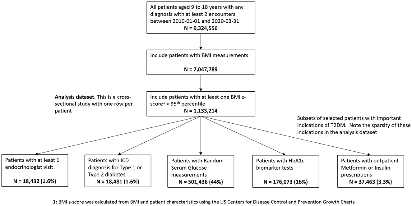
Figure 1. Data specification for pediatric patients at risk of T2DM in Optum™ EHR database. The bottom row shows the number of patients having the model study characteristics for the pediatric T2DM phenotype for the relevant variables.

2.2.2 Gibbs Monte Carlo sampling

We used JAGS [21] as the baseline approach for comparison with all other methods since it uses the simplest method of Metropolis-based MCMC [39]. Our initial baseline objective was to reproduce the Hubbard et al. model using the same methods they employed but against a different EHR database. We used the same JAGS LCA model published by Hubbard et al. in their GitHub supplement⁶.

2.2.3 Hamiltonian Monte Carlo sampling

We used Stan MC [22] for an alternative MCMC comparison given that Stan makes use of a different Metropolis-based sampling method to JAGS and particularly for our model employs marginalization of discrete latent variables. Stan uses a variant of Hamiltonian Monte Carlo called 'No U-turn Sampler (NUTS)' [40]. This approach includes a gradient optimization step, so it cannot sample discrete latent parameters in the way JAGS can. Instead, Stan MC integrates the posterior distribution over the discrete classes [41], so this is a useful comparison to the discrete sampling Gibbs approach. We translated the JAGS model directly to a Stan model using similar sampling notation and had reasonable results (Table 4) though Stan does have various helper functions, for example, log-sum-exp and the target log-probability increment statement.

Table 4

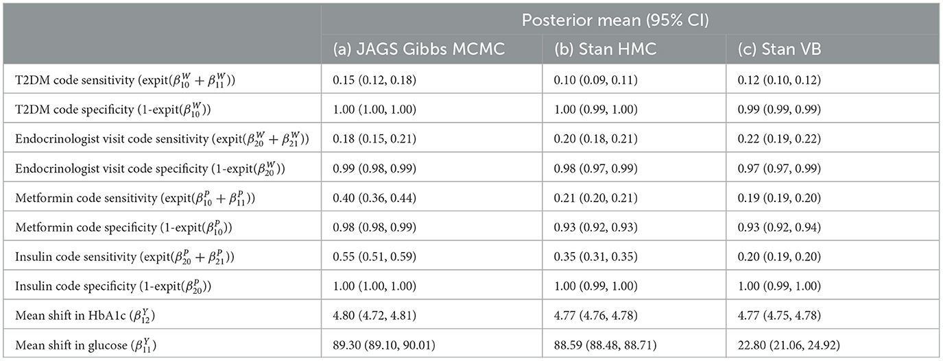
Table 4. Comparison of composite LCA/regression model results for clinical attributes.

2.2.4 Variational inference

We used Stan Automatic Differentiation VB [26] for comparison with MCMC. In Stan, there is only one implementation of variational inference, the automatic differentiation approach [27]. We found this was challenging for the composite Bayes LCA/regression model. For both Stan MCMC and VB, we used the same Stan model definition⁷. There is a lack of closed-form solutions implemented in R or Python for variational Bayes LCA.

Figure 2 illustrates a common problem with current VB implementations. There are two hyperparameters for stopping, a maximum number of ELBO calculation iterations and a difference threshold (delta) between iteration t and t−1. In Figure 2, we can see that the argmin{ELBO} has effectively converged after approximately 30,000 iterations but we have set maximum iterations to 200,000 and the threshold tolerance relatively low meaning it is never reached so the algorithm continues well past the best estimate it can produce. Unfortunately, there is no way a priori to know what a suitable threshold tolerance should be as ELBO values are unbounded or the effective number of iterations for ELBO convergence as this depends on various factors including model specification and algorithm tuning. However, the variational approach uses significantly less computer memory than MCMC. With this EHR phenotyping model on our computer system, VB used 1.8GB vs. 37GB of RAM memory for a three-chain MCMC.

Figure 2

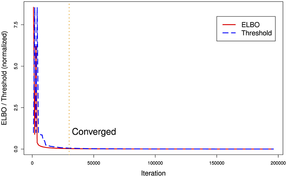
Figure 2. Runtime ELBO (solid) and threshold delta (dashed) for all iterations. ELBO and threshold have been normalized to the same scale. We can see there is a diminishing return after approximately 30,000 iterations (vertical dotted line). In this example, the algorithm ran for over a day longer than it needed to (on a Dell XPS computer with 8-cpu Intel core i9 and 64 GB RAM memory) in finding the best posterior estimate it could generate.

2.2.5 Comparison with maximum likelihood approach

We used the R package clustMD [15] to compare a maximum likelihood (MLE) clustering approach to Bayesian LCA. clustMD employs a mixture of Gaussian distributions to model the latent variable and an expectation maximization (EM) algorithm to estimate the latent cluster means. It also employs Monte Carlo EM for categorical data. clustMD supports mixed data so is appropriate in our context. To use clustMD, the data must be reordered to have continuous variables first, followed by ordinal variables and then nominal variables. For our data, the computational runtime was approximately 50% of JAGS MCMC, approximately 62 h.

3 Results

A Dell XPS 7590 laptop with an 8 CPU Intel core i9 processor and 64GB memory was used for this study. This computer also has an NVIDIA GeForce GTX 1650 GPU, but it was not used.

3.1 Logistic regression model

Eleven VB implementations were compared against several MCMC implementations. We used JAGS MCMC as our baseline comparison. The mean of the model coefficients averaged over the 5-fold was compared with the MCMC baseline (Figure 3). The heatmap indicates some variables are more challenging across multiple VB methods, for example, skin thickness and insulin, which have a high proportion of zero values (Table 5). CAVI, however, returns coefficients very close to MCMC, and it returns comparable empirical performance (Figure 4) and computational performance (Figure 5). Overall, the closed-form conditionally conjugate VB methods outperform automatic black-box VB implementations both empirically and computationally. Two Python implementations from the package PyMC3, Full-rank ADVI (FRADVI) and Amortized Stein Variational Gradient Descent (ASVGD) could not be configured to produce reasonable results despite a full grid search across their algorithm hyperparameters.

Figure 3

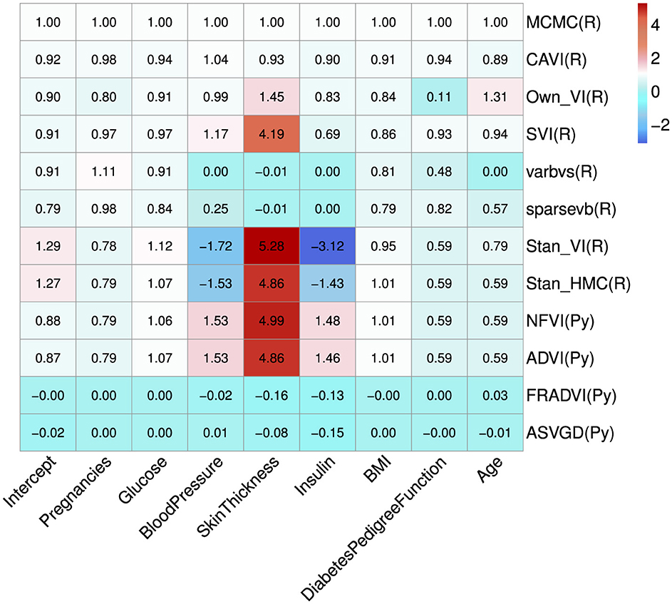
Figure 3. Average coefficient mean over the 5-fold normalized to the MCMC model (top row). The cell values are calculated by simply normalizing the true values to the corresponding MCMC true value, that is, $cell=\frac{{\beta }_{true}}{{\beta }_{mcmc}}$. The programming environment is indicated in the y-axis labels by R for R programming and Py for Python programming. All standard errors are less than 0.25 of the mean SE for MCMC.

Table 5

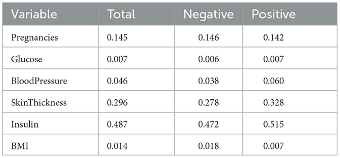
Table 5. Proportions of zero values in Pima Indians data in total, for the negative Outcome class and for the positive Outcome class.

Figure 4

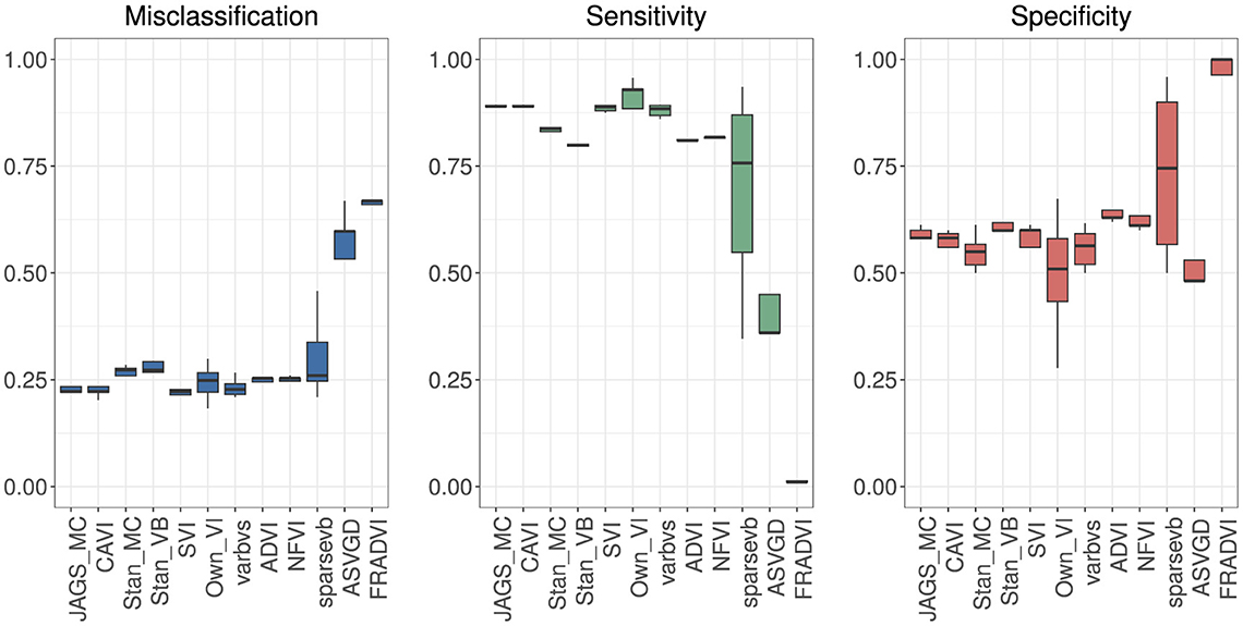
Figure 4. Predictive performance for 5-fold cross-validation. MCMC is the baseline. The purpose of running cross-validation is to check the model stability across data slices.

Figure 5

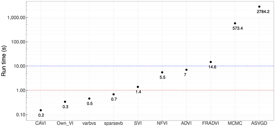
Figure 5. Computational run times in seconds. Four methods produced sub-second performance (red dotted line), and three had <10 s run time (blue dotted line). These are very significant improvements compared with MCMC (~10 min). All results are using the Dell XPS 7590 laptop mentioned at the start of this section.

It is notable from Figure 3 that the sign for some coefficients is different to that of MCMC, especially the coefficients for blood pressure and insulin for both Stan implementations. The resulting data in Table 6 show that JAGS MCMC returns negative coefficients for both variables whereas Stan HMC and VB return positive coefficients for these variables (apart from one Stan VB fold). We used flat priors for this model so perhaps more informative priors are required for the Stan methods, as mentioned in Chapter 1 of the Stan user's guide. These implementations might also be more influenced by data containing a high proportion of zeros.

Table 6

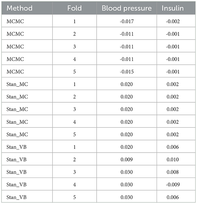
Table 6. Resulting coefficients for 5-fold for blood pressure and insulin comparing MCMC with Stan_MC and Stan_VB.

The empirical predictive performances closest to MCMC were CAVI, SVI [29], and varbvs [31] (Figure 4). All three are mean-field methods that require analytical derivation of the optimization ELBO in contrast to automatic methods ADVI and NFVI [32]. All five methods remained reasonably stable across the five cross-validation folds.

3.2 Composite Bayes LCA/regression model

The baseline results using the Northeast region subset of Optum™ obtained from JAGS were close to the Hubbard et al. results (Table 7). The differences in biomarker shift can be explained by the wider patient geographic catchment and differences in missing data for PEDSnet and Optum™. The striking difference for Endocrinologist visit sensitivity could be due to the much smaller proportion of such visits occurring in the Optum™ data, that is, 63.43% in PEDSnet EHR vs. 5.9% in Optum™ EHR. Following these results, we are confident in the extensibility of the model to the same disease area with different EHR data. Unfortunately, the computational performance is poor using JAGS. For example, a subset of ~38,000 observations taking 16 h to run.

Table 7

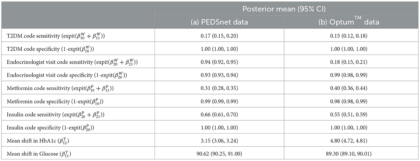
Table 7. Comparison of Optum™ results with Hubbard et al. PEDSnet using the same JAGS LCA model published in Hubbard et al. GitHub [17].

We tested posterior diagnostics, goodness-of-fit diagnostics, and the empirical performance of the composite model. Stan has comprehensive posterior diagnostics available via the posterior [42] and bayesplot [43] R packages. The loo R package [44] provides goodness-of-fit diagnostics based on Pareto Smoothed Importance Sampling (PSIS) [45], leave-one-out cross-validation, and the Watanabe-Akaike/Widely Applicable information criterion (WAIC) [44, 46].

3.2.1 Posterior diagnostics

The posterior diagnostics plots for the biomarkers in Figure 6 show that, for (a) MCMC, we see no evidence of collinearity and the posterior means appear close to those we obtained with JAGS (b). The mcmc pairs plot for VB appears reasonable for HbA1c but not for the glucose biomarker rpg_b_int prior. There appears to be a correlation between the glucose priors and the expected value for glucose is far from that obtained with MCMC (Table 4). We were unable to fully explain this correlation and the glucose mode far from that reported by MCMC. We made several amendments to the model specification along with algorithm hyperparameter tuning that all returned the same effect for glucose. Since there is a single chain for VB, there is only the top triangular set, which represents 100% of the posterior samples. This type of plot does not communicate the relative variances of the posteriors.

Figure 6

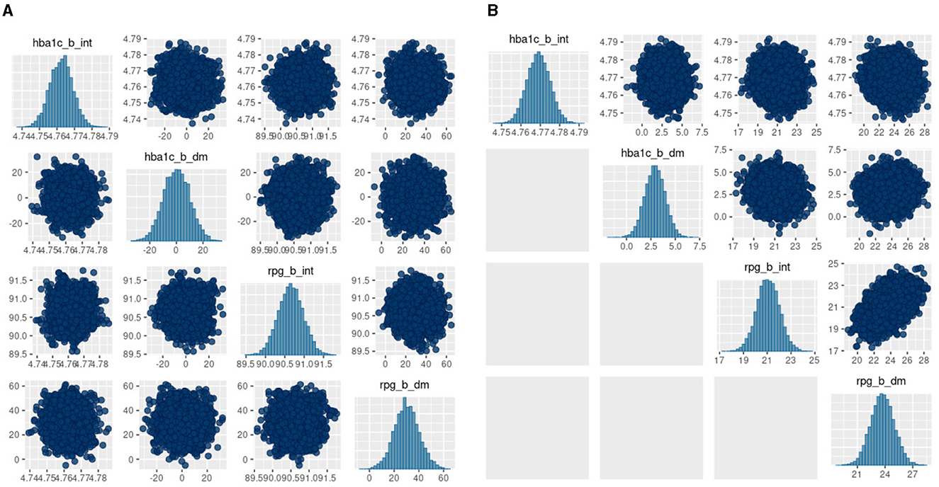
Figure 6. bayesplot pairs plots for (A) Stan HMC and (B) Stan VB for the two biomarkers (HbA1c and random plasma glucose, RPG). Each biomarker contains two priors as defined in the model specification (Table 2). The b_int prior is the multivariate normal, ${\beta }_j^Y$, representing a biomarker test result for normal, non-diabetes patients and the b_dm prior encodes known information on predictive accuracy containing values corresponding to a ROC AUC of 0.95. as described in Hubbard et al. Sections 2.2 and 2.5 [17].

3.2.2 Goodness of fit

We used approximate leave-one-out cross-validation from the R loo package to evaluate the goodness of fit for the model. loo uses log-likelihood point estimates from the model to measure its predictive accuracy against training samples generated by Pareto Smoothed Importance Sampling (PSIS) [45]. The PSIS shape parameter k is used to assess the reliability of the estimate. If k < 0.5, the variance of the importance ratios is finite and the central limit theorem holds. If k is between 0.5 and 1, the variance of the importance ratios is infinite but the mean exists. If k> 1, the variance and mean of the importance ratios do not exist. The results for the two biomarkers (Figure 7) show all of the n=38,000 observations are in a k < 0.5 range. It appears VB performs approximately as well as MCMC in the context of the PSIS metric.

Figure 7

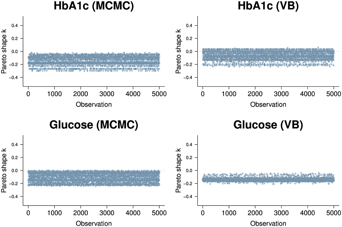
Figure 7. PSIS plots for the two biomarkers, HbA1c (top row) and Random Glucose (bottom row) under MCMC (left) and VB (right). Both biomarkers are well below k=0.5. The HbA1c biomarker is slightly worse for VB with a segment of observations above 0 but is well within good territory. The random glucose biomarker appears better in VB compared to MCMC, but we know that the expected value obtained by VB for glucose is not as close to the true value obtained by MCMC.

3.2.3 Empirical performance

The model sensitivity analysis for the indicator variables shows good agreement with MCMC (Table 4). The mean shift estimates for biomarkers glucose variable under ADVI.

3.2.4 Comparison with maximum likelihood approach

For clustMD, we take cluster 1 as the T2DM class as it is the minority cluster. The cluster means parallel coordinate plot in Figure 8A indicates similar HbA1c (4.81) and glucose (89.9) levels compared to the Bayesian model. Cluster 1 has a significantly larger variance (Figure 8B) possibly due to the high imbalance of the T2DM positive class in the data.

Figure 8

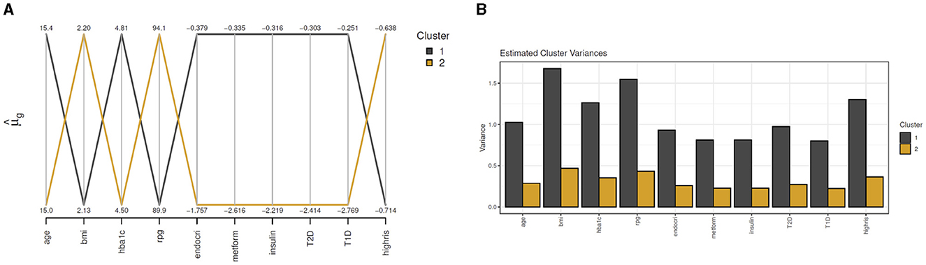
Figure 8. clustMD plots running 2 latent clusters. (A) shows a parallel coordinates plot for all variables, (B) shows the cluster variances for all variables.

4 Discussion

We compared the use of VB and MCMC for Bayesian latent class analysis and logistic regression models with the objective of scaling a composite LCA/regression patient phenotyping model proposed by Hubbard et al. [17] We compared a number of alternative methods for estimating parameters in the model to identify if the intrinsic computational limitations from MCMC can be overcome in a real-world clinical setting using VB. We compared VB and MCMC for logistic regression and latent class analysis for similar clinical settings with two data sets, Pima Indians' diabetes and Optum™ EHR diabetes data. We set out some practical issues in using VB compared to MCMC for these methods on these data such as model stability, data size (primarily in terms of large N), and mixed discrete and continuous data. Some practical guidance included balancing accuracy and runtime via hyperparameter settings and amelioration of label switching via setting constraints on the priors to ensure close vicinity to the clinically expected solution. For Bayes LCA, we found a lack of closed-form VB implementations currently available so we used black-box automatic approaches. We find automatic black-box VB methods as implemented both for the baseline Pima Indian logistic regression model and the Optum™ EHR composite LCA/regression model are complex to configure and very sensitive to model and prior definition, algorithm hyperparameters and choice of gradient optimiser. The composite Bayes LCA/regression model was significantly more challenging to implement, but it was possible to achieve reasonable results with careful model specification and hyperparameter tuning. This, however, results in an iterative trial-and-error approach that we find can sometimes be more cumbersome than running a multi-chain MCMC. This study has a number of limitations. In the Optum™ EHR case study, we have not fully explained why the VB posterior prior values for random plasma glucose are so different to those obtained via MCMC (both JAGS and Stan). This result is a potential question for further work. Further limitations are the exploration of examples where some (but not all) methods run into issues and a discussion as to why this may be, for example, Kucukelbir et. al., allude to potential avenues in Section 5 of their ADVI paper [26] and Dhaka et. al. list several challenges with black-box approaches to VB [47]. Further work could also explore how these methods compare for not only large n but also large p, such as for genetic data. Since data sparsity is an important aspect of clinical data, we feel a comprehensive investigation of this area is warranted. We also deliberately restricted our comparison to Bayesian methods so that prior information could be incorporated, so we did not include detailed comparisons with machine learning or frequentist methods. The Pima Indians case study demonstrated that the closed-form conditionally conjugate mean-field approach to VB, even though it has many simplifying assumptions, performed best of the VB approaches, excelling both computationally and in achieving posterior accuracy comparable to the MCMC gold standard for that data set.

Data availability statement

The original contributions presented in the study are included in the article/Supplementary material, further inquiries can be directed to the corresponding author.

Author contributions

BB: Conceptualization, Data curation, Investigation, Methodology, Project administration, Software, Validation, Writing – original draft, Writing – review & editing. AO'H: Conceptualization, Project administration, Supervision, Validation, Writing – review & editing. MG: Conceptualization, Project administration, Supervision, Validation, Writing – review & editing.

Funding

The author(s) declare that no financial support was received for the research, authorship, and/or publication of this article.

Conflict of interest

The authors declare that the research was conducted in the absence of any commercial or financial relationships that could be construed as a potential conflict of interest.

Publisher's note

All claims expressed in this article are solely those of the authors and do not necessarily represent those of their affiliated organizations, or those of the publisher, the editors and the reviewers. Any product that may be evaluated in this article, or claim that may be made by its manufacturer, is not guaranteed or endorsed by the publisher.

Supplementary material

The Supplementary Material for this article can be found online at: https://www.frontiersin.org/articles/10.3389/fams.2024.1302825/full#supplementary-material

Footnotes

1. ^https://www.kaggle.com/datasets/uciml/pima-indians-diabetes-database

2. ^See Section 8: Latent Discrete Parameters in the Stan Users Guide.

3. ^See Section 13: Variational Inference Algorithm: ADVI in the Stan User's Guide.

4. ^https://github.com/tommasorigon/logisticVB

5. ^M+1 is to account for the regression intercept.

6. ^https://github.com/rhubb/Latent-phenotype/

7. ^See Supplementary Appendix S2 for the Stan LCA model details.

References

1. Boulanger B, Carlin BP. How and why Bayesian statistics are revolutionizing pharmaceutical decision making. Clinical Researcher. (2021) 703:20.

Google Scholar

2. He T, Belouali A, Patricoski J, Lehmann H, Ball R, Anagnostou V, et al. Trends and opportunities in computable clinical phenotyping: a scoping review. J Biomed Inform. (2023) 140:104335. doi: 10.1016/j.jbi.2023.104335

PubMed Abstract | Crossref Full Text | Google Scholar

3. Hripcsak G, Albers DJ. Next-generation phenotyping of Electronic Health Records. J Am Med Inform Assoc. (2013) 20:117–21. doi: 10.1136/amiajnl-2012-001145

PubMed Abstract | Crossref Full Text | Google Scholar

4. Xia Z, Sheinson D. P30 combining real-world and randomized controlled trial survival data using bayesian methods. Value in Health. (2022) 25:S293. doi: 10.1016/j.jval.2022.04.040

Crossref Full Text | Google Scholar

5. Carlin BP, Nollevaux F. Bayesian complex innovative trial designs (CIDs) and their use in drug development for rare disease. J Clini Pharmacol. (2022) 62:S56–71. doi: 10.1002/jcph.2132

PubMed Abstract | Crossref Full Text | Google Scholar

6. Alsowaida YS, Kubiak DW, Dionne B, Kovacevic MP, Pearson JC. Vancomycin area under the concentration-time curve estimation using bayesian modeling versus first-order pharmacokinetic equations: a quasi-experimental study. Antibiotics. (2022) 11:1239. doi: 10.3390/antibiotics11091239

PubMed Abstract | Crossref Full Text | Google Scholar

7. Cuker A, Buckley B, Mousseau MC, Barve AA, Haenig J, Bussel JB. Early initiation of second-line therapy in primary immune thrombocytopenia: insights from real-world evidence. Ann Hematol. (2023) 102:1–8. doi: 10.1007/s00277-023-05289-0

PubMed Abstract | Crossref Full Text | Google Scholar

8. Yang S, Varghese P, Stephenson E, Tu K, Gronsbell J. Machine learning approaches for electronic health records phenotyping: a methodical review. J Am Med Inform Assoc. (2023) 30:367–81. doi: 10.1093/jamia/ocac216

PubMed Abstract | Crossref Full Text | Google Scholar

9. Geyer CJ. Practical Markov Chain Monte Carlo. Statist Sci. (1992) 7:473-483. doi: 10.1214/ss/1177011137

Crossref Full Text | Google Scholar

10. Murphy KP. Machine Learning: A Probabilistic Perspective. Cambridge, MA: MIT Press. (2012).

Google Scholar

11. Song Z, Hu Y, Verma A, Buckeridge DL, Li Y. Automatic phenotyping by a seed-guided topic model. In: Proceedings of the 28th ACM SIGKDD Conference on Knowledge Discovery and Data Mining. (2022) p. 4713–4723. Available at: https://dl.acm.org/doi/proceedings/10.1145/3534678

Google Scholar

12. Li Y, Nair P, Lu XH, Wen Z, Wang Y, Dehaghi AAK, et al. Inferring multimodal latent topics from electronic health records. Nat Commun. (2020) 11:2536. doi: 10.1038/s41467-020-16378-3

PubMed Abstract | Crossref Full Text | Google Scholar

13. Hughes DM. García-Finana M, Wand MP. Fast approximate inference for multivariate longitudinal data. Biostatistics. (2023) 24:177–92. doi: 10.1093/biostatistics/kxab021

PubMed Abstract | Crossref Full Text | Google Scholar

14. Lanza ST, Rhoades BL. Latent class analysis: an alternative perspective on subgroup analysis in prevention and treatment. Preven Sci. (2013) 14:157–68. doi: 10.1007/s11121-011-0201-1

PubMed Abstract | Crossref Full Text | Google Scholar

15. McParland D, Gormley IC. Model based clustering for mixed data: clustMD. Adv Data Anal Classif . (2016) 10:155–69. doi: 10.1007/s11634-016-0238-x

Crossref Full Text | Google Scholar

16. White A, Murphy TB. BayesLCA: An R package for Bayesian latent class analysis. J Stat Softw. (2014) 61:1–28. doi: 10.18637/jss.v061.i13

Crossref Full Text | Google Scholar

17. Hubbard RA, Huang J, Harton J, Oganisian A, Choi G, Utidjian L, et al. A Bayesian latent class approach for EHR-based phenotyping. Stat Med. (2019) 38:74–87. doi: 10.1002/sim.7953

PubMed Abstract | Crossref Full Text | Google Scholar

18. Metropolis N, Ulam S. The Monte Carlo method. J Am Stat Assoc. (1949) 44:335–41. doi: 10.1080/01621459.1949.10483310

PubMed Abstract | Crossref Full Text | Google Scholar

19. Resnik P, Hardisty E. Gibbs Sampling for the Uninitiated. (2010).

Google Scholar

20. Roy V. Convergence diagnostics for Markov Chain Monte Carlo. Ann Rev Stat Appl. (2020) 7:387–412. doi: 10.1146/annurev-statistics-031219-041300

Crossref Full Text | Google Scholar

21. Hornik K, Leisch F, Zeileis A, Plummer M. JAGS: A program for analysis of Bayesian graphical models using Gibbs sampling. In: Proceedings of the 3rd International Workshop on Distributed Statistical Computing. (2003). p. 1–10. Available at: https://www.r-project.org/conferences/DSC-2003/Proceedings/

Google Scholar

22. Carpenter B, Gelman A, Hoffman MD, Lee D, Goodrich B, Betancourt M, et al. Stan: A probabilistic programming language. J Stat Softw. (2017) 76:1. doi: 10.18637/jss.v076.i01

PubMed Abstract | Crossref Full Text | Google Scholar

23. Jordan MI, Ghahramani Z, Jaakkola TS, Saul LK. An introduction to variational methods for graphical models. Mach Learn. (1999) 37:183–233. doi: 10.1023/A:1007665907178

Crossref Full Text | Google Scholar

24. Blei DM, Kucukelbir A, McAuliffe JD. Variational inference: a review for statisticians. J Am Stat Assoc. (2017) 112:859–77. doi: 10.1080/01621459.2017.1285773

Crossref Full Text | Google Scholar

25. Hoffman MD, Blei DM, Wang C, Paisley J. Stochastic variational inference. J Mach Learn Res. (2013) 14:1303–47.

Google Scholar

26. Kucukelbir A, Tran D, Ranganath R, Gelman A, Blei DM. Automatic differentiation variational inference. J Mach Learn Res. (2017) 18:1–45.

Google Scholar

27. Kucukelbir A, Ranganath R, Gelman A, Blei D. Automatic variational inference in Stan. In: Advances in Neural Information Processing Systems (2015). p. 28. Available at: https://papers.nips.cc/paper_files/paper/2015

PubMed Abstract | Google Scholar

28. Smith JW, Everhart JE, Dickson W, Knowler WC, Johannes RS. Using the ADAP learning algorithm to forecast the onset of diabetes mellitus. In: Proceedings of the Annual Symposium on Computer Application in Medical Care. Bethesda, MD: American Medical Informatics Association (1988). p. 261.

Google Scholar

29. Durante D, Rigon T. Conditionally conjugate mean-field variational Bayes for logistic models. Stat Sci. (2019) 34:472–85. doi: 10.1214/19-STS712

PubMed Abstract | Crossref Full Text | Google Scholar

30. Ray K. Szabó B. Variational Bayes for high-dimensional linear regression with sparse priors. J Am Stat Assoc. (2022) 117:1270–81. doi: 10.1080/01621459.2020.1847121

Crossref Full Text | Google Scholar

31. Carbonetto P, Zhou X, Stephens M. varbvs: Fast variable selection for large-scale regression. arXiv [preprint] arXiv:170906597. (2017). doi: 10.48550/arXiv.1709.06597

Crossref Full Text | Google Scholar

32. Salvatier J, Wiecki TV, Fonnesbeck C. Probabilistic programming in Python using PyMC3. PeerJ Comp Sci. (2016) 2:e55. doi: 10.7717/peerj-cs.55

Crossref Full Text | Google Scholar

33. Rezende D, Mohamed S. Variational inference with normalizing flows. In: International Conference on Machine Learning. New York: PMLR (2015). p. 1530–1538.

Google Scholar

34. Liu Q, Wang D. Stein variational gradient descent: a general purpose bayesian inference algorithm. In: Advances in Neural Information Processing Systems 29 (NIPS 2016). (2016). p. 29. Available at: https://proceedings.neurips.cc/paper/2016

Google Scholar

35. Hadjadj S, Coisne D, Mauco G, Ragot S, Duengler F, Sosner P, et al. Prognostic value of admission plasma glucose and HbA1c in acute myocardial infarction. Diabet Med. (2004) 21:305–10. doi: 10.1111/j.1464-5491.2004.01112.x

PubMed Abstract | Crossref Full Text | Google Scholar

36. Wallace PJ, Shah ND, Dennen T, Bleicher PA, Crown WH. Optum Labs: building a novel node in the learning health care system. Health Aff . (2014) 33:1187–94. doi: 10.1377/hlthaff.2014.0038

PubMed Abstract | Crossref Full Text | Google Scholar

37. Dagenais S, Russo L, Madsen A, Webster J, Becnel L. Use of real-world evidence to drive drug development strategy and inform clinical trial design. Clini Pharmacol Therap. (2022) 111:77–89. doi: 10.1002/cpt.2480

PubMed Abstract | Crossref Full Text | Google Scholar

38. Kuczmarski RJ. 2000 CDC Growth Charts for the United States: methods and development (No. 246) 246 Department of Health and Human Services, Centers for Disease Control and Prevention. Hyattsville, MA: National Center for Health Statistics. (2002).

PubMed Abstract | Google Scholar

39. Geman S, Geman D. Stochastic relaxation, Gibbs distributions, and the Bayesian restoration of images. IEEE Trans Pattern Anal Mach Intell. (1984) 6:721–41. doi: 10.1109/TPAMI.1984.4767596

PubMed Abstract | Crossref Full Text | Google Scholar

40. Hoffman MD, Gelman A. The No-U-Turn sampler: adaptively setting path lengths in Hamiltonian Monte Carlo. J Mach Learn Res. (2014) 15:1593–623.

Google Scholar

41. Yackulic CB, Dodrill M, Dzul M, Sanderlin JS, Reid JA. A need for speed in Bayesian population models: a practical guide to marginalizing and recovering discrete latent states. Ecol Appl. (2020) 30:e02112. doi: 10.1002/eap.2112

PubMed Abstract | Crossref Full Text | Google Scholar

42. Bürkner PC, Gabry J, Kay M, Vehtari A. posterior: Tools for Working with Posterior Distributions. In: R Package Version 1.4.1. (2023). Available at: https://mc-stan.org/posterior/ (accessed October 20, 2023).

Google Scholar

43. Gabry J, Mahr T. bayesplot: plotting for Bayesian models. In: R package Version. (2017).

Google Scholar

44. Vehtari A, Gelman A, Gabry J. Practical Bayesian model evaluation using leave-one-out cross-validation and WAIC. Stat Comput. (2017) 27:1413–32. doi: 10.1007/s11222-016-9696-4

Crossref Full Text | Google Scholar

45. Vehtari A, Simpson D, Gelman A, Yao Y, Gabry J. Pareto smoothed importance sampling. arXiv [preprint] arXiv:150702646. (2015). doi: 10.48550/arXiv.1507.02646

Crossref Full Text | Google Scholar

46. Magnusson M, Vehtari A, Jonasson J, Andersen M. Leave-one-out cross-validation for Bayesian model comparison in large data. In: International Conference on Artificial Intelligence and Statistics. New York: PMLR (2020). p. 341–351.

Google Scholar

47. Dhaka AK, Catalina A, Welandawe M, Andersen MR, Huggins J, Vehtari A. Challenges and opportunities in high dimensional variational inference. Adv Neural Inf Process Syst. (2021) 34:7787–98.

PubMed Abstract | Google Scholar