Improving passengers’ attitudes toward safety and unreliable train operations: analysis of a mathematical model of fractional order

In this study, we aimed to explore the dynamics of rail passengers’ negative attitudes that can be influenced by safety concerns and unreliable train operations. We mainly formulated and analyzed a mathematical model of fractional order and derived an optimal control problem considering the Caputo fractional order derivative. In the analysis part of the model, we proved that the solutions of the model for the dynamical system are non-negative and bounded, and determined the passengers’ negative attitude-free and negative attitude persistence equilibrium points of the model. Both the local and global stabilities of these equilibrium points were examined. Furthermore, we verified the conditions necessary for the existence of optimal control strategies. We then proceeded to analyze the proposed control strategies, which aim to prevent negative attitudes and improve the attitudes of passengers who have already developed negative attitudes. Finally, we conducted numerical simulations to examine the effects of these control strategies. The results revealed that protecting passengers from developing negative attitudes and improving the attitudes of those who have already developed such attitudes are crucial for improving the overall attitude of railway passengers. These measures can effectively address any negative experiences caused by safety concerns and unreliable train operations.

1 Introduction

Railway transportation plays a significant role in enhancing market accessibility and facilitating efficient travel for both passengers and goods. The progress of railway development in developed countries has been remarkable, with advanced infrastructure, efficient operations, and continuous technological advancements. However, the progress of railway transportation in developing nations encounters notable difficulties due to inadequate operation and maintenance of railway infrastructure (1). These difficulties contribute to a growing concern regarding the escalation in passengers’ negative attitudes toward railway services (2). Understanding the control strategies behind these negative attitudes is crucial for improving service quality and addressing passengers’ concerns.

The quality of service offered by public transit can be understood by measuring its performance according to the experiences of its riders (3). Several factors influence passengers’ attitudes toward railway transportation, including service quality, safety concerns, a lack of effective communication, frequent breakdowns, overcrowding, and reliability of operation (4). Insufficient communication during disruptions or emergencies can lead to frustration and further dissatisfaction among passengers. Passengers often feel helpless and uninformed, which escalates their dissatisfaction and contributes to negative attitudes toward train services (5).

A decline in passenger satisfaction and an increase in negative attitudes can lead to a decrease in ridership, ultimately affecting the revenue and viability of railway operations (6). Lower customer satisfaction can also lead to a decline in public trust and support, hindering the growth and development of the train industry (7). It is, therefore, crucial to thoroughly examine the dynamics behind passengers’ negative attitudes to gain valuable insights for policymakers and railway operators, enabling them to make well-informed decisions and implement effective measures to improve the overall passenger experience.

To better describe and analyze various aspects of a real-world problem in various disciplines, including science and engineering, mathematical modeling can serve as a powerful tool for representing the problem by using mathematical equations, formulas, and algorithms. This can be observed, for instance, by examining its application in various contexts (8–10).

The authors discussed how mathematical modeling can help identify the key factors that contribute to the dynamics of real-life situations by analyzing the stability of equilibrium points. The classic autonomous ordinary differential equations representing evolutionary systems have no memory, as their solution is independent of the previous instant (11). However, the fractional order differential equations, in contrast, incorporate the memory effect of an evolutionary system, such as passengers’ attitudes. In the context of rail passengers, memory effects can play a significant role in shaping their attitudes. These effects refer to the influence of past experiences and interactions on the present attitude of individuals. Furthermore, memory effects that impact the dynamics include the persistence of negative experiences, recency bias, confirmation bias, social influence, and expectation formation.

A fractional order model means a representation of a system described by a fractional differential equation or a system of such Equation (12). Mathematicians have developed several approaches for fractional derivatives, such as Grunwald-Letnikov, Riemann-Liouville, and Caputo’s fractional derivatives. The Riemann-Liouville method results in initial conditions that include the limiting values of the Riemann-Liouville fractional derivatives at the lower bound $t=a$ , and these types of initial conditions lack a recognized physical interpretation. Applied engineering problems require the formulation of a fractional order model with the use of physically interpretable initial conditions, such as $X\left(a\right),X^{\prime }\left(a\right),X^{″}\left(a\right),$and so on. Caputo’s approach enables the formulation of initial conditions for fractional order differential equations at the lower terminal $t=a$ (12).

The Caputo fractional derivative approach is another mathematical technique that can be employed for evolutionary systems with memory effect. The application of this approach has been dealt with in various contexts (13–17). Bhalekar et al. (18) considered the dynamics of the fractional order systems involving non-local derivative operators on singular points in the solution trajectories of the systems. The study investigated the behavior of the trajectories when the eigenvalues $\lambda$ are at a specified stable region and examined the existence of singular points in the trajectories of such systems in a given region. Echenausía-Monroy et al. (19) investigated a physical interpretation of fractional-order derivatives in a jerk system using an electronic approach based on unstable dissipative systems (UDSs) and a saturated non-linear function (SNLF). The results of the analysis revealed that, when the orders of the fractional integration are considered, the areas of the generated attractor are modified with respect to the integer-order dynamic. Zhou et al. (20) clarified the physical process for fractional dynamical systems. The dynamics in fractional order systems have been discussed extensively for presenting possible guidance in the field of applied mathematics and interdisciplinary science.

Motivated by the concepts discussed above, in this study, we constructed a Caputo fractional derivative compartmental modeling approach to analyze the dynamics of passengers’ negative attitudes toward railway transportation. These advanced analytical techniques enable us to gain insights into the underlying factors contributing to negative attitudes and explore strategies for improving passengers’ attitudes.

The remainder of this article is structured as follows: in section 2, we present some basic terminologies necessary for the formulation of mathematical models of fractional order. The formulation of integer and fractional order models is given in section 3. Section 4 presents the optimal control problem, followed by the numerical simulation in section 5. Finally, in section 6, we conclude the article with a summary and discuss future work.

2 Basic terminology of fractional order calculus

The following concepts of fractional order calculus will serve as a foundation for constructing the fractional order model in this study:

Definition 1: The Caputo fractional order derivative of order $\vartheta$ for a function $f\in C^n$ is defined by Vargas-De-León (17) and Petrás (21).

$\begin{array}{ll}{\mathrm{C}}_{D_t^{\vartheta }f\left(t\right)=\frac{1}{\Gamma \left(\mathrm{n}-\vartheta \right)}{{\displaystyle \int }}_0^t{f}^n\left(\zeta \right)\frac{{\left(t-\zeta \right)}^{n-\vartheta }}{t-\zeta }d\zeta ,n-1<\vartheta \le n\in N}& (1)\end{array}$

Note:

$\begin{array}{ll}{\mathrm{C}}_{D_t^{\vartheta }f\left(t\right)\mathrm{tends\; to}\dot{f}\left(t\right)as\vartheta \to 1}& (2)\end{array}$

Definition 2: The Caputo fractional order integral of order $\mathrm{\hspace{0.33em}}\mathrm{\hspace{0.33em}}\vartheta >0$ for a function $f\in C^n$ is defined by Vargas-De-León (17) and Petrás (21).

$\begin{array}{ll}{\mathrm{C}}_{I_t^{\vartheta }f\left(t\right)=\frac{1}{\Gamma \left(\vartheta \right)}{{\displaystyle \int }}_0^{t}f\left(\zeta \right)\frac{{\left(t-\zeta \right)}^{\vartheta }}{t-\zeta }d\zeta ,0<\vartheta \langle 1,t\rangle 0}& (3)\end{array}$

Definition 3: Let ${\gamma }_1>0,{\gamma }_2>0$ be positive parameters, then the Mittag–Leffler function is defined by Mainardi (22), Fernandez and Husain (23), and Özarslan and Fernandez (24).

$\begin{array}{ll}{E}_{{\gamma }_{1,}{\gamma }_2}\left(t\right)={\displaystyle \sum }_{m=1}^{\infty }\frac{t^m}{\Gamma \left({\gamma }_1\mathrm{m}+{\gamma }_2\right)}& (4)\end{array}$

Definition 4: Suppose ${\gamma }_2=1$ is the constant parameter. Then, the Mittag–Leffler function is defined by Mainardi (22) and Özarslan and Fernandez (24).

$\begin{array}{ll}{E}_{{\gamma }_1,1}\left(t\right)={\displaystyle \sum }_{m=1}^{\infty }\frac{t^m}{\Gamma \left({\gamma }_1\mathrm{m}+1\right)}=E_{{\gamma }_1}\left(t\right)& (5)\end{array}$

Definition 5: A constant number ${\theta }^{\ast }$ is identified as an equilibrium point of the Caputo-fractional order model when

$\begin{array}{ll}{\mathrm{C}}_{D_t^{\vartheta }\theta \left(t\right)=f\left(t\mathrm{,}\theta \left(t\right)\right),\vartheta \in \left[0\mathrm{,}1\right]\mathrm{if\; and\; only\; if}f\left(t\mathrm{,}{\theta }^{\ast }\right)=0}& (6)\end{array}$

Proposition 1: The Laplace transform of the Caputo fractional order derivative with order $\vartheta ,$ $n-1<\vartheta \le n,n\in N$ is given by $L\left(D_t^{\vartheta }h\right)\left(s\right)=s^{\vartheta }H\left(s\right)-{\displaystyle \sum }_{k=1}^{n-1}{s}^{\vartheta -k-1}{h}^k\left(0\right)$ , where $H\left(s\right)$ is the Laplace transform of the function $h\left(t\right)$ .

Proposition 2: The Laplace transformation of the two-parameter functions of the Mittag–Leffler case is given by Balatif et al. (25).

$\mathrm{L}\left({\mathrm{t}}^{{\gamma }_2-1}{\mathrm{E}}_{{\gamma }_{1,}{\gamma }_2}\left(\pm \gamma {\mathrm{t}}^{{\gamma }_1}\right)\right)\left(\mathrm{s}\right)=\frac{{\mathrm{s}}^{{\gamma }_{1-}{\gamma }_2}}{{\mathrm{s}}^{{\gamma }_1}\mp \gamma }$

Proposition 3 (Generalized Mean Value theorem): Suppose $h\left(t\right)\in \mathcal{L}\left[0\mathrm{,}{T}_f\right]$ and ^C $D_t^{\vartheta }h\left(t\right)\in \mathcal{L}\left[0\mathrm{,}{T}_f\right]$ for $\vartheta \in \left(0\mathrm{,}1\right]$ . Then, the theorem states that $h\left(t\right)=h\left(0\right)+\frac{1}{\Gamma \left(\vartheta \right)}$ ^C $D_t^{\vartheta }h\left(\zeta \right)t^{\vartheta },$ where $\zeta \in \left[0\mathrm{,}t\right]$ for each $t$ such that $0<t\le T_f$ .

Note: These statements follow from Proposition 3.

a. The function $h$ is non-decreasing for all $t\in \left[0\mathrm{,}{T}_f\right]$ , if ^C $D_t^{\vartheta }h\left(t\right)\ge 0.$

b. The function $h$ is non-increasing for all $t\in \left[0\mathrm{,}{T}_f\right]$ , if ^C $D_t^{\vartheta }h\left(t\right)\le 0.$

Proposition 4: Suppose $g\left(t\right)\in L^{\infty }\left(ℝ\right)\cap \mathcal{F}\left(ℝ\right)$ and $\in ℝ,$ $n-1<\vartheta \le n,n\in N$ . Then, the following conditions hold

$\begin{array}{ll}{(}^C{D}_t^{\vartheta }{I}^{\vartheta }g)\left(t\right)=g\left(t\right).& (\mathrm{})\end{array}$

a. $(I^{\vartheta }$ $C{D}_t^{\vartheta }g)\left(t\right)=g\left(t\right)-{\displaystyle \sum }_{k=0}^{n-1}\frac{t^k}{k!}{g}^k\left(0\right).$

b. Specifically, if $0<\vartheta <1$ , then $(I^{\vartheta }$C $D_t^{\vartheta }g)\left(t\right)=g\left(t\right)-g\left(0\right).$

c. For a constant function $g\left(t\right)=b$ then $C{D}_t^{\vartheta }\left(b\right)=0.$

3 Models’ formulation

3.1 Description and assumptions of the models

To analyze the dynamics of the passengers’ negative attitudes toward railway transportation, we divided the total number of passengers, denoted by M(t) at a given time t, into five distinct mutually exclusive classes: susceptible passengers who can develop negative attitudes whenever they are exposed, which is denoted by S(t), passengers who are exposed to negative attitudes due to perceived safety concerns and unreliable operation of train services, which is denoted by E(t), passengers who developed negative attitude due to safety concerns, which is denoted by $I_S\left(t\right),$ passengers who developed negative attitudes due to unreliable train operation, which is denoted by $I_U\left(t\right),$ and passengers whose negative attitudes changed, which is denoted by R(t). The passengers who developed negative attitudes due to unreliable train operation may have encountered trains running late or not adhering to the schedule, leading to frustration and dissatisfaction.

$\begin{array}{ll}M\left(t\right)=S\left(t\right)+E\left(t\right)++I_S\left(t\right)+I_U\left(t\right)+R\left(t\right).& (7)\end{array}$

Acquiring a negative attitude from another passenger is not influenced by the number of passengers around, and susceptible individuals within the population acquire negative attitudes from other passengers at a standard incidence rate given by

$\begin{array}{ll}{\lambda }_{\mathrm{SC}}\left(\mathrm{t}\right)=\frac{\beta }{M}\left({\rho }_1{I}_S\left(t\right)+{\rho }_2{I}_U\left(\mathrm{t}\right)\right).& (8)\end{array}$

where

${\rho }_1$ is the relative effect of passengers with negative attitudes due to safety concerns;

${\rho }_2$ is the relative effect of passengers with negative attitudes due to unreliable train operation; and

$\beta$ is the transmission rate of negative attitude.

To construct the Caputo fractional order model for the transmission dynamics of negative attitudes among passengers in a population, certain key assumptions need to be considered.

A portion $\mathrm{\hspace{0.33em}}q$ of susceptible passengers who were exposed to negative attitude, i.e., S(t) transfers to the $I_S\left(t\right)$ , a portion of passengers who developed negative attitudes due to safety concerns at a rate $\varpi$ , while the remaining portion $1-q$ joins $I_U\left(t\right),$ a portion of passengers who developed negative attitudes due to unreliable train operation at the same rate.

Passengers with negative attitude due to safety concerns $I_S\left(t\right)$ and those with negative attitude due to unreliable train operation $I_U\left(t\right)\mathrm{\hspace{0.33em}}$progress to the portion of passengers whose negative attitudes $R\left(t\right)$ at the rates ${\alpha }_1$ and ${\alpha }_2$ , respectively. The rate $\eta$ is the progression of individuals from the $I_S$ portion to $I_U$ . Other parameters and state variables are stated in Tables 1, 2.

Table 1

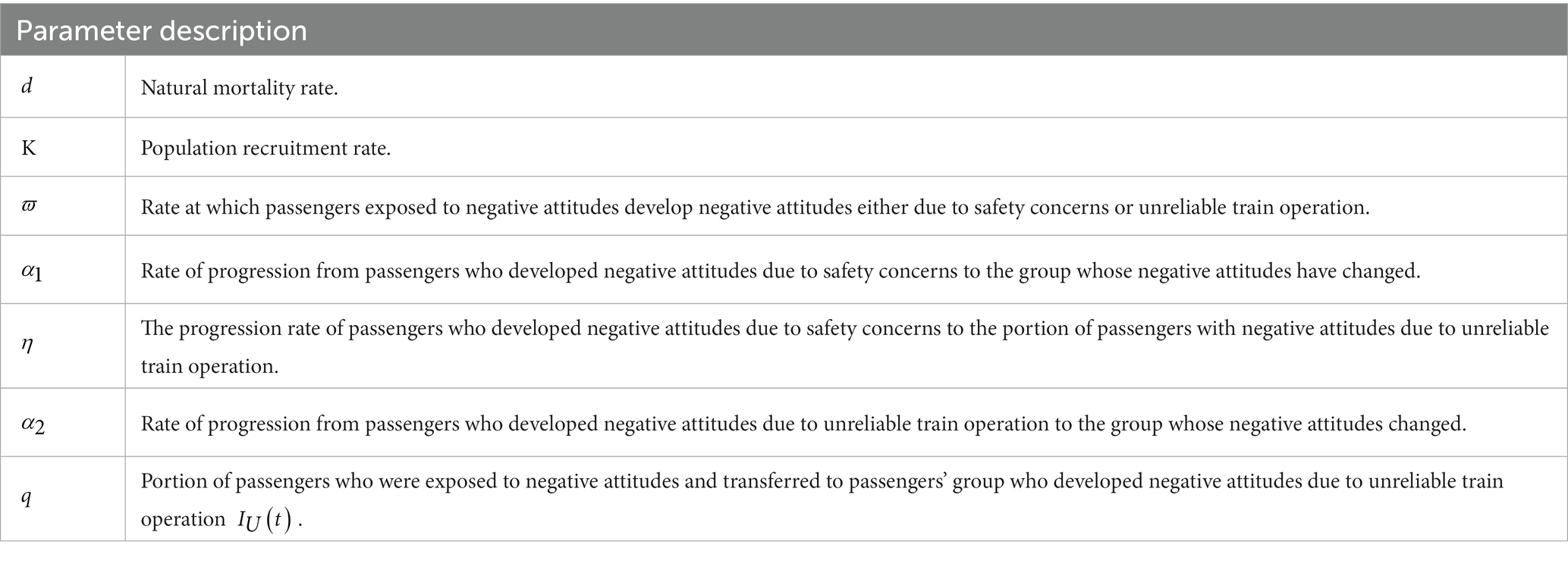
Table 1. Description of parameters.

Table 2

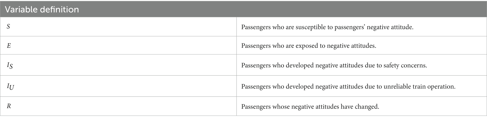
Table 2. Definitions of state variables.

The population flow diagram, which is based on the model descriptions and assumptions given above, illustrates how the negative attitude of passengers disseminates among the population.

3.2 Integer order model

The integer order model, a system of non-linear first-order ordinary differential equations, is based on the population flow diagram given in Figure 1 and represents the evolution of passengers’ negative attitudes, which is given by

$\frac{dS}{dt}={\rm K}-\left({\lambda }_{SC}+d\right)S$

$\frac{dE}{dt}={\lambda }_{SC}\mathrm{S}-\left(d+\varpi \right)E$

$\frac{\mathrm{d}{I}_S}{\mathrm{dt}}=\left(1-\mathrm{q}\right)\varpi E-\left(\mathrm{d}+{\alpha }_1+\eta \right)I_S$

$\frac{\mathrm{d}{I}_U}{\mathrm{dt}}=q\varpi E+\eta I_S-\left(\mathrm{d}+{\alpha }_2\right)I_U$

$\begin{array}{ll}\frac{dR}{dt}={\alpha }_1{I}_S+{\alpha }_2{I}_U-dR& (9)\end{array}$

$\begin{array}{ll}\text{subject to }S\left(0\right)>0,\mathrm{\hspace{0.33em}}E\left(0\right)\ge 0,I_S\left(0\right)\ge 0\mathrm{\hspace{0.33em}}\mathrm{\hspace{0.33em}}{I}_U\left(0\right)\ge 0,\mathrm{and}\mathrm{\hspace{0.33em}}R\left(0\right)\ge 0& (10)\end{array}$

Figure 1

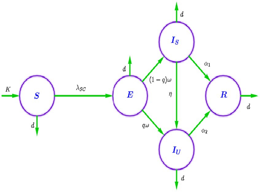
Figure 1. The passengers’ flow diagram.

3.3 Fractional order model

In this subsection, we reformulated the transmission dynamics of passengers’ negative attitude model (Equation 9). This is done by using Caputo derivatives, which allows us to incorporate memory effects and gain a deeper understanding of the evolution of passengers’ negative attitudes. The mathematical representation of this fractional order model can be observed in Equation 11.

${\mathrm{C}}_{D_t^{\vartheta }S=K^{\vartheta }-\left({\lambda }_{SC}+d^{\vartheta }\right)S}$

${\mathrm{C}}_{D_t^{\vartheta }E={\lambda }_{SC}\mathrm{S}-\left(d^{\vartheta }+{\varpi }^{\vartheta }\right)E}$

${\mathrm{C}}_{D_t^{\vartheta }{I}_S=q^{\vartheta }{\varpi }^{\vartheta }E-\left(d^{\vartheta }+{\alpha }_1^{\vartheta }+{\eta }^{\vartheta }\right)I_S}$

${\mathrm{C}}_{D_t^{\vartheta }{I}_U=q^{\vartheta }{\varpi }^{\vartheta }E+{\eta }^{\vartheta }{I}_S-\left({\mathrm{d}}^{\vartheta }+{\alpha }_2^{\vartheta }\right)I_U}$

$\begin{array}{ll}{\mathrm{C}}_{D_t^{\vartheta }R={\alpha }_1^{\vartheta }{I}_S+{\alpha }_2^{\vartheta }{I}_U-d^{\vartheta }R}& (11)\end{array}$

The initial data for the proposed fractional order model (Equation 11) is demonstrated by

$\begin{array}{ll}S\left(0\right)\ge 0,\mathrm{\hspace{0.33em}}\mathrm{\hspace{0.33em}}E\left(0\right)\ge 0,\mathrm{\hspace{0.33em}}\mathrm{\hspace{0.33em}}{I}_S\left(0\right)\ge 0,\mathrm{\hspace{0.33em}}\mathrm{\hspace{0.33em}}{I}_U\left(0\right)\ge 0,R\left(0\right)\ge 0& (12)\end{array}$

The analysis of the fractional order model given in Equation 11 is presented in the Supplementary material, where theorem 1 shows the non-negativity and boundedness of the model, and theorem 2 demonstrates the existence and uniqueness of solution of the model. The equilibrium points and basic reproduction bombers are calculated in section 3. The local stability of the negative attitude free equilibrium point is addressed in theorem 3, while the global stability of equilibrium points is illustrated in theorems 5 and 6.

4 Optimal control problem

The negative attitude of rail passengers is a complex behavior that can be influenced by various factors. In the context of unreliable train operations and safety concerns, it is important to address this negative attitude to improve the overall passenger experience.

The prevention control strategy aims to reduce the number of susceptible passengers by addressing the factors contributing to negative attitudes. For example, improving train operations and implementing safety measures can help create a positive passenger experience and reduce the likelihood of developing negative attitudes. By focusing on prevention, the goal is to minimize the number of passengers who become exposed to negative attitudes and subsequently develop negative attitudes.

On the other hand, the improvement control strategy focuses on addressing the negative attitudes of passengers who developed negative attitudes and helping them to change their attitudes. Assisting in the process of changing their negative attitudes can be done through various measures, such as providing information, assistance, and support to passengers who have developed negative attitudes. By actively addressing and improving these negative attitudes, the goal is to facilitate the process of changing their negative attitudes and ultimately reducing the overall number of passengers who develop negative attitudes.

By combining both prevention and improvement control strategies, the researchers proposed a comprehensive approach to managing rail passengers’ negative attitudes. This approach acknowledges the importance of addressing the root causes of negative attitudes through prevention while recognizing the need to support and improve the attitudes of those who have already developed negative attitudes. Through this control design, the researchers aimed to create a positive rail travel experience for passengers, which in turn can enhance customer satisfaction and loyalty.

We presented three control strategies that depend on time and are designed to modify the fractional order model (Equation 11). These strategies are represented by the Lebesgue controlling functions ${\mathrm{u}}_1\left(\mathrm{t}\right)$ , $\mathrm{\hspace{0.33em}}\mathrm{\hspace{0.33em}}{\mathrm{u}}_2\left(\mathrm{t}\right)$ , and ${\mathrm{u}}_3\left(\mathrm{t}\right)$ , with 0 $\le {\mathrm{u}}_1\left(\mathrm{t}\right),{\mathrm{u}}_2\left(\mathrm{t}\right),{\mathrm{u}}_3\left(\mathrm{t}\right)\le 1\mathrm{\hspace{0.33em}}$ .

These functions serve as measures of control and are defined as follows:

1. The measure to prevent passengers’ negative attitudes is aimed at minimizing the effective contact rate, and it is represented by the control measure $u_1\left(t\right)$ . This measure involves taking actions to enhance the management of congestion during train operations and improve the daily operation of trains by ensuring punctuality and regularity.

2. The time-dependent control measures represented by $u_2\left(t\right)$ and $u_3\left(t\right)$ are improvement strategies for passengers who developed negative attitudes as a result of safety concerns and unreliable train operations, respectively.

The new reformulation of the Caputo fractional order model’s optimal control problem (Equation 11) is based on the control variables mentioned earlier.

${\mathrm{C}}_{D_t^{\vartheta }S=K^{\vartheta }-\left(\left(1-u_1\left(t\right)\right)\frac{{\beta }^{\vartheta }\left({\rho }_1^{\vartheta }{I}_S+{\rho }_2^{\vartheta }{I}_U\right)}{M}+d^{\vartheta }\right)S}$

${\mathrm{C}}_{D_t^{\vartheta }E=\left(1-u_1\left(t\right)\right)\frac{{\beta }^{\vartheta }\left({\rho }_1^{\vartheta }{I}_S+{\rho }_2^{\vartheta }{I}_U\right)}{M}-\left(d^{\vartheta }+{\varpi }^{\vartheta }\right)E}$

${\mathrm{C}}_{D_t^{\vartheta }{I}_S=\left(1-q^{\vartheta }\right){\varpi }^{\vartheta }E-\left(d^{\vartheta }+{\eta }^{\vartheta }+u_2\left(t\right){\alpha }_1^{\vartheta }\right)I_S}$

${\mathrm{C}}_{D_t^{\vartheta }{I}_U=q^{\vartheta }{\varpi }^{\vartheta }E+{\eta }^{\vartheta }{N}_S-\left(d^{\vartheta }+u_3\left(t\right){\alpha }_2^{\vartheta }\right)I_U}$

$\begin{array}{ll}{\mathrm{C}}_{D_t^{\vartheta }R=u_2\left(t\right){\alpha }_1^{\vartheta }{I}_S+u_3\left(t\right){\alpha }_2^{\vartheta }{I}_U-d^{\vartheta }R}& (13)\end{array}$

with initial data $\mathrm{\hspace{0.33em}}S\left(0\right)>0$ , $E\left(0\right)\ge 0,I_S\left(0\right)\ge 0$ , $\mathrm{\hspace{0.33em}}{I}_U\left(0\right)\ge 0$ , and $\mathrm{\hspace{0.33em}}R\left(0\right)\ge 0,$and the controlling set is ${\Delta }_C=\left\{\left(u_1\left(t\right)\mathrm{,}{u}_2\left(t\right)\mathrm{,}{u}_3\left(t\right)\right):0\le u_1\left(t\right)\mathrm{,}{u}_2\left(t\right)\mathrm{,}{u}_3\left(t\right)\le 1\mathrm{,}t\in \left[0\mathrm{,}{T}_f\right]\right\}$ , where $T_f\mathrm{\hspace{0.33em}}$is the final time of implementing control measures.

The aim of the control problem is to minimize the number of people who are exposed to and develop negative attitudes while increasing the number of individuals whose negative attitudes change, taking into account the cost of implementing control strategies. To achieve this, we formulated an objective function that represents the goal of reducing the number of individuals who have already developed negative attitudes in the population.

$\begin{array}{ll}J\left(u_1\mathrm{,}{u}_2\mathrm{,}{u}_3\right)={{\displaystyle \int }}_0^{T_f}\left({\chi }_{1}E+{\chi }_2{\mathrm{I}}_S+{\chi }_3{\mathrm{I}}_U+\frac{{\Gamma }_1}{2}{u}_1^2+\frac{{\Gamma }_2}{2}{u}_2^2+\frac{{\Gamma }_3}{2}{u}_3^2\right)dt& (14)\end{array}$

To manage the number of individuals who developed negative attitudes and the associated costs of implementing prevention and improvement control strategies, we strived to minimize $u_1\mathrm{\hspace{0.33em}}\left(t\right),u_2\mathrm{\hspace{0.33em}}\left(t\right)$ , and $u_3\mathrm{\hspace{0.33em}}\left(t\right)$ while considering the system (Equation 14) as a constraint.

In this section, the value $T_f$ represents the final time, while the coefficients ${\chi }_1,{\chi }_2,$and ${\chi }_3\mathrm{\hspace{0.33em}}$are positive weight constants. The measures $\frac{{\Gamma }_1}{2},\frac{{\Gamma }_2}{2}$ , and $\frac{{\Gamma }_3}{2}$ represent the relative costs of prevention and improvement corresponding to the controls $u_1,u_2,$and $\mathrm{\hspace{0.33em}}{u}_3$ , respectively. Additionally, these measures help to balance the units of the integrand.

The objective is to locate the optimal values for the controls $U=\left(u_1\mathrm{,}{u}_2\mathrm{,}{u}_3\right)$ , denoted as $U^{\ast }=\left(u_1^{\ast }\mathrm{,}{u}_2^{\ast }\mathrm{,}{u}_3^{\ast }\right),$ to achieve the desired state trajectories $S^{\ast },E^{\ast },I_S^{\ast },I_U^{\ast },$and $R^{\ast }$ that are solutions of (Equation 14) over a given time interval $\left[0\mathrm{,}{T}_f\right]$ . These state trajectories should also satisfy the initial data and minimize the objective function.

In the cost functional, the term $\mathrm{\hspace{0.33em}}{\chi }_{1}E\mathrm{\hspace{0.33em}}$represents the cost related to individuals exposed to negative attitudes, the term ${\chi }_2{\mathrm{I}}_S$ refers to the cost related to individuals who developed negative attitudes due to safety concerns, and the term ${\chi }_3{\mathrm{I}}_U$ represents the cost related to individuals who developed negative attitudes due to unreliable train operation.

Additionally, ${\chi }_i$ (where $i=1,2,3$ ) are positive constants that represent the cost of implementing the three strategies to control, and ${\Gamma }_i$ (where $i=1,2,3$ ) is the corresponding effort made to minimize the dissemination of negative attitudes toward these strategies. $T_f$ represents the duration for which the control measures are applied.

The aim is to determine the optimal control variable $u\left(t\right)$ that minimizes the objective function $\underset{\overline{u}\in \overline{U}}{\min }J\left(\overline{u}\right)$ , which is subject to the new optimal control dynamical system given in Equation 13 with the initial data.

The vector $\overline{u}=\mathrm{\{}{u}_1\mathrm{,}{u}_2\mathrm{,}{u}_3\mathrm{)}$ is the vector that controls the system, and the set

$\begin{array}{ll}\overline{U}=\left\{\overline{u}\in {\left(L^{\infty }\left(\left[0\mathrm{,}{T}_f\right]\right)\right)}^3\mathrm{,}0\le u_i\le 1\mathrm{,}i=1\mathrm{,}2\mathrm{,}3\mathrm{,}\right\}& (15)\end{array}$

is a closed and bounded set of controls that are admissible.

4.1 Existence and optimality of the control strategies

The fractional order dynamical system (Equation 11) with (Equation 12) can be rewritten as follows:

${\mathrm{C}}_{D_t^{\vartheta }Y=G\left(t\mathrm{,}Y\left(t\right)\right)+H\left(t\mathrm{,}Y\left(t\right)\right)\overline{u},0\le t\le T_f,}$

$Y\left(t\right)=Y_0,$ where $Y\left(t\right)=\left(S\left(t\right)\mathrm{,}E\left(t\right)\mathrm{,}{I}_S\left(t\right)\mathrm{,}{I}_U\left(t\right)\mathrm{,}R\left(t\right)\right)$ represents the state variables of the dynamical system, and $u\left(t\right)=(u_1\left(t\right),u_2\left(t\right),u_3\left(t\right)$ represents the control functions or variables in the control problem mentioned in Equation 13. The functions G and H are given as follows:

$G\left(t\mathrm{,}Y\left(t\right)\right)=\left[\begin{array}{c}{\mathrm{K}}^{\vartheta }-\left(\frac{{\beta }^{\vartheta }\left({\rho }_1^{\vartheta }{I}_S+{\rho }_2^{\vartheta }{I}_U\right)}{M}+d^{\vartheta }\right)S\\ \frac{{\beta }^{\vartheta }\left({\rho }_1^{\vartheta }{I}_S+{\rho }_2^{\vartheta }{I}_U\right)}{M}\mathrm{S}-\left(d^{\vartheta }+{\varpi }^{\vartheta }\right)E\\ \left(1-q^{\vartheta }\right){\varpi }^{\vartheta }E-\left(d^{\vartheta }+{\eta }^{\vartheta }\right)I_S\\ q^{\vartheta }{\varpi }^{\vartheta }E+{\eta }^{\vartheta }{I}_S-\left({\mathrm{d}}^{\vartheta }\right)I_U\\ -d^{\vartheta }R\end{array}\right]$

$H\left(t\mathrm{,}Y\left(t\right)\right)=\left[\begin{array}{ccc}\frac{{\beta }^{\vartheta }\left({\rho }_1^{\vartheta }{I}_S+{\rho }_2^{\vartheta }{I}_U\right)}{M}\mathrm{S}& 0& 0\\ -\frac{{\beta }^{\vartheta }\left({\rho }_1^{\vartheta }{I}_S+{\rho }_2^{\vartheta }{I}_U\right)}{M}\mathrm{S}& 0& 0\\ 0& -{\alpha }_1^{\vartheta }{I}_S& 0\\ 0& 0& -{\alpha }_2^{\vartheta }{I}_U\\ 0& {\alpha }_1^{\vartheta }{I}_S& {\alpha }_1^{\vartheta }{I}_S\end{array}\right]$

To establish the existence of the three optimal control strategies, we need to verify the following conditions:

• The control trajectories have at least one feasible solution.

• The set of admissible controls is convex, bounded, and closed.

• The function represented by $G\left(t\mathrm{,}Y\left(t\right)\right)+H\left(t\mathrm{,}Y\left(t\right)\right)$ is bounded with respect to both the state variables and the controlling variables.

• The expression ${\chi }_{1}E+{\chi }_2{\mathrm{I}}_S+{\chi }_3{\mathrm{I}}_U+\frac{{\Gamma }_1}{2}{u}_1^2+\frac{{\Gamma }_2}{2}{u}_2^2+\frac{{\Gamma }_3}{2}{u}_3^2$ is convex on the set of admissible controls $\overline{U}$ .

According to the definitions mentioned in the manuscript, the conditions can be expressed as follows:

If we consider control functions with values $\mathrm{\hspace{0.33em}}{u}_1=1,$ $\mathrm{\hspace{0.33em}}{u}_2=0$ , and $\mathrm{\hspace{0.33em}}{u}_3=0$ within the admissible control set $\overline{U}$ defined in Equation 15 and the solution $Y=\left(S\mathrm{,}E{\mathrm{,I}}_{\mathrm{S}}\mathrm{,}{I}_U\mathrm{,}R\right)$ of the fractional order model (Equation 11) with given initial data, then the set of all feasible solutions for the control problem is not empty. Furthermore, based on the definition of the admissible control set $\overline{U},$ this control set is bounded, closed, and convex. Additionally, according to the existence and uniqueness criteria for model (Equation 11), the solutions of model (Equation 13) are unique and bounded because $0\le u_i\le 1,$ for $i=1,2,3.$

Theorem 7: The function defined by $G\left(t\mathrm{,}Y\left(t\right)\right)+H\left(t\mathrm{,}Y\left(t\right)\right)\overline{u}$ satisfies the solution.

$\overline{Y}=\left(S\mathrm{,}E{\mathrm{,I}}_A{\mathrm{,I}}_C\mathrm{,}R\right)$ such that

$\begin{array}{ll}\left|\right|G\left(t\mathrm{,}\overline{Y}\right)+H\left(t\mathrm{,}\overline{Y}\right)\mathrm{}\left|\right|\le \max \left(k_1\mathrm{,}{k}_2\right)\left(\left|\right|\overline{Y}\left|\right|+\left|\right|\overline{u}\left|\right|\right)& (16)\end{array}$

where $k_1=\max \left(\begin{array}{l}1+{\beta }^{\vartheta }\left({\rho }_1^{\vartheta }+{\rho }_2^{\vartheta }\right)+d^{\vartheta }\mathrm{,}{d}^{\vartheta }+{\varpi }^{\vartheta }\mathrm{,}{d}^{\vartheta }\\ +d_1^{\vartheta }+{\eta }^{\vartheta }+{\alpha }_1^{\vartheta }\mathrm{,}{d}^{\vartheta }+d_2^{\vartheta }+{\alpha }_2^{\vartheta }\mathrm{,}{d}^{\vartheta }\end{array}\right),$ and $k_2=\max \left({\beta }^{\vartheta }\left({\rho }_1^{\vartheta }+{\rho }_2^{\vartheta }\right)\mathrm{,}{\eta }^{\vartheta }\mathrm{,}1\right)$ .

Proof: Let us consider the matrix $G\left(t\mathrm{,}Y\left(t\right)\right)$ in a rewritten form.

$\begin{array}{l}G\left(t\mathrm{,}Y\left(t\right)\right)=\\ \left[\begin{array}{ccccc}D& 0& 0& 0& 0\\ \frac{{\beta }^{\vartheta }\left(\begin{array}{l}{\rho }_1^{\vartheta }{I}_A\\ +{\rho }_2^{\vartheta }{I}_C\end{array}\right)}{M}& -\left(\begin{array}{l}{d}^{\vartheta }+\\ {\varpi }^{\vartheta }\end{array}\right)& 0& 0& 0\\ 0& \left(\begin{array}{l}1-\\ q^{\vartheta }\end{array}\right){\varpi }^{\vartheta }& \left(\begin{array}{l}{d}^{\vartheta }+d_1^{\vartheta }+\\ {\eta }^{\vartheta }+{\alpha }_1^{\vartheta }\end{array}\right)& 0& 0\\ 0& q^{\vartheta }{\varpi }^{\vartheta }& {\eta }^{\vartheta }& \left(\begin{array}{l}{d}^{\vartheta }+d_2^{\vartheta }\\ +{\alpha }_2^{\vartheta }\end{array}\right)& 0\\ 0& 0& {\alpha }_1^{\vartheta }& {\alpha }_2^{\vartheta }& -d^{\vartheta }\end{array}\right]\left[\begin{array}{c}S\\ E\\ {\mathrm{I}}_{\mathrm{S}}\\ I_U\\ R\end{array}\right],\end{array}$

where $D=\frac{{\mathrm{K}}^{\vartheta }}{S}-\frac{{\beta }^{\vartheta }\left({\rho }_1^{\vartheta }{I}_S+{\rho }_2^{\vartheta }{I}_U\right)}{M}$ .

Given the definition of the matrix $G\left(t\mathrm{,}Y\left(t\right)\right)$ , we can see that ${\mathrm{K}}^{\vartheta }\le S$ . Additionally, considering the bounded nature of the solution, we demonstrate that

$\left|\right|G\left(t\mathrm{,}\overline{Y}\right)\left|\right|\le \max \left(\begin{array}{l}1+{\beta }^{\vartheta }\left({\rho }_1^{\vartheta }+{\rho }_2^{\vartheta }\right)+d^{\vartheta }\mathrm{,}{d}^{\vartheta }+{\varpi }^{\vartheta }\mathrm{,}{d}^{\vartheta }\\ +d_1^{\vartheta }+{\eta }^{\vartheta }+{\alpha }_1^{\vartheta }\mathrm{,}{d}^{\vartheta }+d_2^{\vartheta }+{\alpha }_2^{\vartheta }\mathrm{,}{d}^{\vartheta }\end{array}\right)\left|\right|\overline{Y}\left|\right|$

By employing a similar procedure, we can demonstrate the following:

$\left|\right|G\left(t\mathrm{,}\overline{Y}\right)\left|\right|\le \max \left({\beta }^{\vartheta }\left({\rho }_1^{\vartheta }+{\rho }_2^{\vartheta }\right)\mathrm{,}{\eta }^{\vartheta }\mathrm{,}1\right)\left|\right|\overline{u}\left|\right|.$

Theorem 8: The function expressed as $\mathbb{V}\left(t\mathrm{,}\overline{Y}\mathrm{,}\overline{u}\right)={\chi }_{1}E+{\chi }_2{\mathrm{I}}_S+{\chi }_3{\mathrm{I}}_U+\frac{{\Gamma }_1}{2}{u}_1^2+\frac{{\Gamma }_2}{2}{u}_2^2+\frac{{\Gamma }_3}{2}{u}_3^2$ is convex within the admissible control region $\overline{U}$ , and there exists a non-negative constant $k$ such that $\mathbb{V}\left(t\mathrm{,}\overline{Y}\mathrm{,}\overline{u}\right)\ge k\overline{u}$ .

Proof: For the function $\mathbb{V}\left(t\mathrm{,}\overline{Y}\mathrm{,}\overline{u}\right)$ , we derived the corresponding Hessian matrix given by

$ℍ=\left[\begin{array}{ccc}2u_1& 0& 0\\ 0& 2u_2& 0\\ 0& 0& 2u_3\end{array}\right].$

Therefore, the matrix $ℍ$ is a positive definite matrix in the admissible control region $\overline{U}$ and hence $\mathbb{V}\left(t\mathrm{,}\overline{Y}\mathrm{,}\overline{u}\right)\mathrm{\hspace{0.33em}}$is strictly convex in $U.$ Let $k=\min \left(\frac{{\Gamma }_1}{2}\mathrm{,}\frac{{\Gamma }_2}{2}\mathrm{,}\frac{{\Gamma }_3}{2}\right),$ then $\begin{array}{l}\mathbb{V}\left(t\mathrm{,}\overline{Y}\mathrm{,}\overline{u}\right)={\chi }_{1}E+{\chi }_2{\mathrm{I}}_{\mathrm{S}}+{\chi }_3{I}_U+\frac{{\Gamma }_1}{2}{u}_1^2+\frac{{\Gamma }_2}{2}{u}_2^2+\frac{{\Gamma }_3}{2}{u}_3^2\\ \ge \frac{{\Gamma }_1}{2}{u}_1^2+\frac{{\Gamma }_2}{2}{u}_2^2+\frac{{\Gamma }_3}{2}{u}_3^2\ge k\left(\frac{{\Gamma }_1}{2}{u}_1^2+\frac{{\Gamma }_2}{2}{u}_2^2+\frac{{\Gamma }_3}{2}{u}_3^2\right)\end{array}$ . Thus, we established the proof.

Theorem 9: There is an optimal control point ${\overline{u}}^{\ast }=\left(u_1^{\ast }\mathrm{,}{u}_2^{\ast }\mathrm{,}{u}_3^{\ast }\right)$ and the model-associated solutions

${\overline{Y}}^{\ast }=\left(S^{\ast }\mathrm{,}{E}^{\ast }\mathrm{,}{N}_S^{\ast }\mathrm{,}{N}_R^{\ast }\mathrm{,}{R}^{\ast }\right)$ that minimize the objective function $J\left(\overline{u}\right)$ on the admissible control set $\overline{U}$ , such that $\underset{\overline{u}\in \overline{U}}{\min }J\left(\overline{u}\right)=J\left({\overline{u}}^{\ast }\right)$ .

The optimality necessary condition: The optimality necessary condition, as stated in Teklu and Terefe (26), is required to be fulfilled by the optimal control problem (Equation 13), and Equation 14 is adapted from Pontryagin’s maximum principle stated in Mandal et al. (13), Ahmed et al. (16), and Teklu and Terefe (27), and it is also fulfilled by changing into a minimizing Hamiltonian function with respect to the control variables $\left(u_1\mathrm{,}{u}_2\mathrm{,}{u}_3\right)$ . The Hamiltonian function corresponding to Equations 13 and 14 is derived as follows:

$\begin{array}{c}H\left(\overline{Y},\overline{u},{\mathrm{K}}^{\vartheta }\right)=\\ {\chi }_{1}E+{\chi }_2{\mathrm{I}}_{\mathrm{S}}+{\chi }_3\mathrm{}{I}_U+\\ \frac{{\Gamma }_1}{2}{u}_1^2+\frac{{\Gamma }_2}{2}{u}_2^2+\frac{{\Gamma }_3}{2}{u}_3^2+{\lambda }_1\\ \left({\mathrm{K}}^{\vartheta }-\left(\begin{array}{l}\left(1-\mathrm{}{u}_1\left(t\right)\right)\\ \mathrm{}\frac{{\beta }^{\vartheta }\left(\begin{array}{l}{\rho }_1^{\vartheta }{I}_S\\ +{\rho }_2^{\vartheta }{I}_U\end{array}\right)}{M}+d^{\vartheta }\end{array}\right)S\right)\\ +{\lambda }_2\left(\begin{array}{l}\left(1-\mathrm{}{u}_1\left(t\right)\right)\\ \mathrm{}\frac{{\beta }^{\vartheta }\left(\begin{array}{l}{\rho }_1^{\vartheta }{I}_S\\ +{\rho }_2^{\vartheta }{I}_U\end{array}\right)}{M}-\left(d^{\vartheta }+{\varpi }^{\vartheta }\right)E\end{array}\right)\\ +{\lambda }_3\left(\begin{array}{l}\left(1-q^{\vartheta }\right){\varpi }^{\vartheta }E-\\ \left(\begin{array}{l}{d}^{\vartheta }+d_1^{\vartheta }+\\ {\eta }^{\vartheta }+u_2\left(t\right){\alpha }_1^{\vartheta }\end{array}\right)I_S\end{array}\right)\\ +{\lambda }_4\left(\begin{array}{l}{q}^{\vartheta }{\varpi }^{\vartheta }E+{\eta }^{\vartheta }{I}_S-\\ \left(\begin{array}{l}{d}^{\vartheta }+d_2^{\vartheta }\\ +u_3\left(t\right){\alpha }_2^{\vartheta }\end{array}\right)I_U\end{array}\right)\\ +{\lambda }_5\left(\begin{array}{l}{u}_2\left(t\right){\alpha }_1^{\vartheta }{I}_S+\\ u_3\left(t\right){\alpha }_2^{\vartheta }{I}_U-d^{\vartheta }R\end{array}\right)\end{array}\text{ (17)}$

where ${\lambda }_1\left(t\right),{\lambda }_2\left(t\right),{\lambda }_3\left(t\right),{\lambda }_4\left(t\right),$ and $\mathrm{\hspace{0.33em}}{\lambda }_5\left(t\right)$ are the co-state variables or adjoint variables.

Theorem 10: Let us give the optimal control solutions $u_i^{\ast }$ for $i=1,2,3$ and the solutions of the optimal control problem (Equation 13) that minimize the objective function (Equation 15) in the admissible control region $\overline{U}$ , then there are functions ${\lambda }_1,{\lambda }_2,{\lambda }_3,{\lambda }_4,$and ${\lambda }_5$ such that

${\mathrm{C}}_{D_t^{\vartheta }{\lambda }_1=\left({\lambda }_1-{\lambda }_2\right)\left(1-u_1\right)\frac{{\beta }^{\vartheta }\left({\rho }_1^{\vartheta }{I}_S+{\rho }_2^{\vartheta }{I}_U\right)}{M}\left(1-\frac{S}{M}\right)+d^{\vartheta }{\lambda }_1}$

${\mathrm{C}}_{D_t^{\vartheta }{\lambda }_2=\left({\lambda }_2-{\lambda }_1\right)\left(1-u_1\right)\frac{{\beta }^{\vartheta }\left({\rho }_1^{\vartheta }{I}_S+{\rho }_2^{\vartheta }{I}_U\right)S}{M^2}+{\lambda }_2\left(d^{\vartheta }+{\varpi }^{\vartheta }\right)-{\lambda }_3\left(1-q^{\vartheta }\right){\varpi }^{\vartheta }-{\lambda }_3{q}^{\vartheta }{\varpi }^{\vartheta }-{\chi }_1}$

${\mathrm{C}}_{\begin{array}{l}{D}_t^{\vartheta }{\lambda }_3=\left({\lambda }_2-{\lambda }_1\right)\left(1-u_1\right)\left(\frac{{\beta }^{\vartheta }\left({\rho }_1^{\vartheta }{I}_S+{\rho }_2^{\vartheta }{I}_U\right)S}{M^2}-{\beta }^{\vartheta }{\rho }_1^{\vartheta }\frac{S}{M}\right)\\ +\left({\lambda }_3-{\lambda }_4\right)\left({\eta }^{\vartheta }+u_2\right)+{\lambda }_{3}B+{\lambda }_4{\alpha }_1^{\vartheta }-{\chi }_2\end{array}}$

${\mathrm{C}}_{D_t^{\vartheta }{\lambda }_4=\left({\lambda }_2-{\lambda }_1\right)\left(1-u_1\right)\left(\frac{{\beta }^{\vartheta }\left({\rho }_1^{\vartheta }{I}_S+{\rho }_2^{\vartheta }{I}_U\right)S}{M^2}-{\beta }^{\vartheta }{\rho }_2^{\vartheta }\frac{S}{M}\right)+\left({\lambda }_4-{\lambda }_5\right)\left({\alpha }_2^{\vartheta }+u_3\right)+{\lambda }_4\left(d^{\vartheta }\right)-{\chi }_3}$

$\begin{array}{ll}{\mathrm{C}}_{D_t^{\vartheta }{\lambda }_5=\left({\lambda }_2-{\lambda }_1\right)\left(1-u_1\right)\frac{{\beta }^{\vartheta }\left({\rho }_1^{\vartheta }{I}_S+{\rho }_2^{\vartheta }{I}_U\right)S}{M^2}+{\lambda }_5{d}^{\vartheta }}& (18)\end{array}$

where $B=\left(d^{\vartheta }+{\alpha }_1^{\vartheta }\right).$

The conditions for the transversality of the system (Equation 18) can be expressed as ${\lambda }_{\mathrm{i}}^{\ast }\left({\mathrm{T}}_{\mathrm{f}}\right)=0$ , $\mathrm{i}=1,2,\dots ,5$ . These conditions are based on the Hamiltonian function $\mathrm{H}$ defined mentioned in Equation 17. Additionally, the optimal control strategy can be determined by

$u_1^{\ast }\left(t\right)=\min \left\{1\mathrm{,}\max [0\mathrm{,}\frac{\left({\lambda }_1-{\lambda }_2\right)}{{\Gamma }_1}\frac{{\beta }^{\vartheta }\left({\rho }_1^{\vartheta }{I}_S+{\rho }_2^{\vartheta }{I}_U\right)S}{M}\right\}$

$u_2^{\ast }\left(t\right)=\min \left\{1\mathrm{,}\max [0\mathrm{,}\frac{\left({\lambda }_3-{\lambda }_5\right)}{{\Gamma }_2}{N}_S\right\}$

$u_2^{\ast }\left(t\right)=\min \left\{1\mathrm{,}\max [0\mathrm{,}\frac{\left({\lambda }_4-{\lambda }_5\right)}{{\Gamma }_3}{N}_R\right\}$

where ${\lambda }_1\left(t\right),{\lambda }_2\left(t\right),{\lambda }_3\left(t\right),{\lambda }_4\left(t\right),{\lambda }_5\left(t\right)$ , and ${\lambda }_6\left(t\right)$ are the co-state variables or adjoint variables and the conditions for transversality that are mentioned earlier.

Proof: The existence of the co-state variables ${\lambda }_1\left(t\right),{\lambda }_2\left(t\right),{\lambda }_3\left(t\right),{\lambda }_4\left(t\right),{\lambda }_5\left(t\right)$ is demonstrated by applying Pontryagin’s maximal principle, as shown in reference (15, 28). Furthermore, the characterization of each optimal control strategy outlined in Equation 13 is achieved by solving the following set of partial differential equations within the interior of the admissible control set $\overline{U}$ as follows:

$\begin{array}{ll}\frac{\partial H}{\partial u_1}=\frac{\partial H}{\partial u_2}=\frac{\partial H}{\partial u_3}=0.& (19)\end{array}$

5 Numerical simulation

In this section, we conducted numerical simulations of model (Equation 11) and control problem (Equation 13) to gain a deeper understanding of the system’s behavior and pinpoint the most efficient optimal control strategies that influence the evolution of passengers’ attitudes. These simulations yield visualizations, enhancing our intuitive grasp of how different factors affect the transmission dynamics and serving as valuable tools for scenario evaluation. We utilized the ODE45 solver in MATLAB 2023a for numerical simulations to capture the dynamics of the passengers’ attitude model. This solver, belonging to the second-order Runge–Kutta family of methods and utilizing either the Euler forward or backward finite difference method, is chosen for its ability to generate accurate and reliable results (29).

5.1 Numerical simulations to show the effect of changing fractional order

Some values of the fractional order $\vartheta$ are taken to check the performance of the proposed model. The simulation curve illustrated in Figures 2A-D indicates how changes in fractional order affect the negative attitudes of passengers toward railway transportation. Based on the results of Figure 2, it can be observed that, when the fractional order decreases, there is a decrease in the numbers of exposed passengers and passengers with negative attitudes due to safety concerns and unreliable train operations. These changes are attributed to the memory effect.

Figure 2

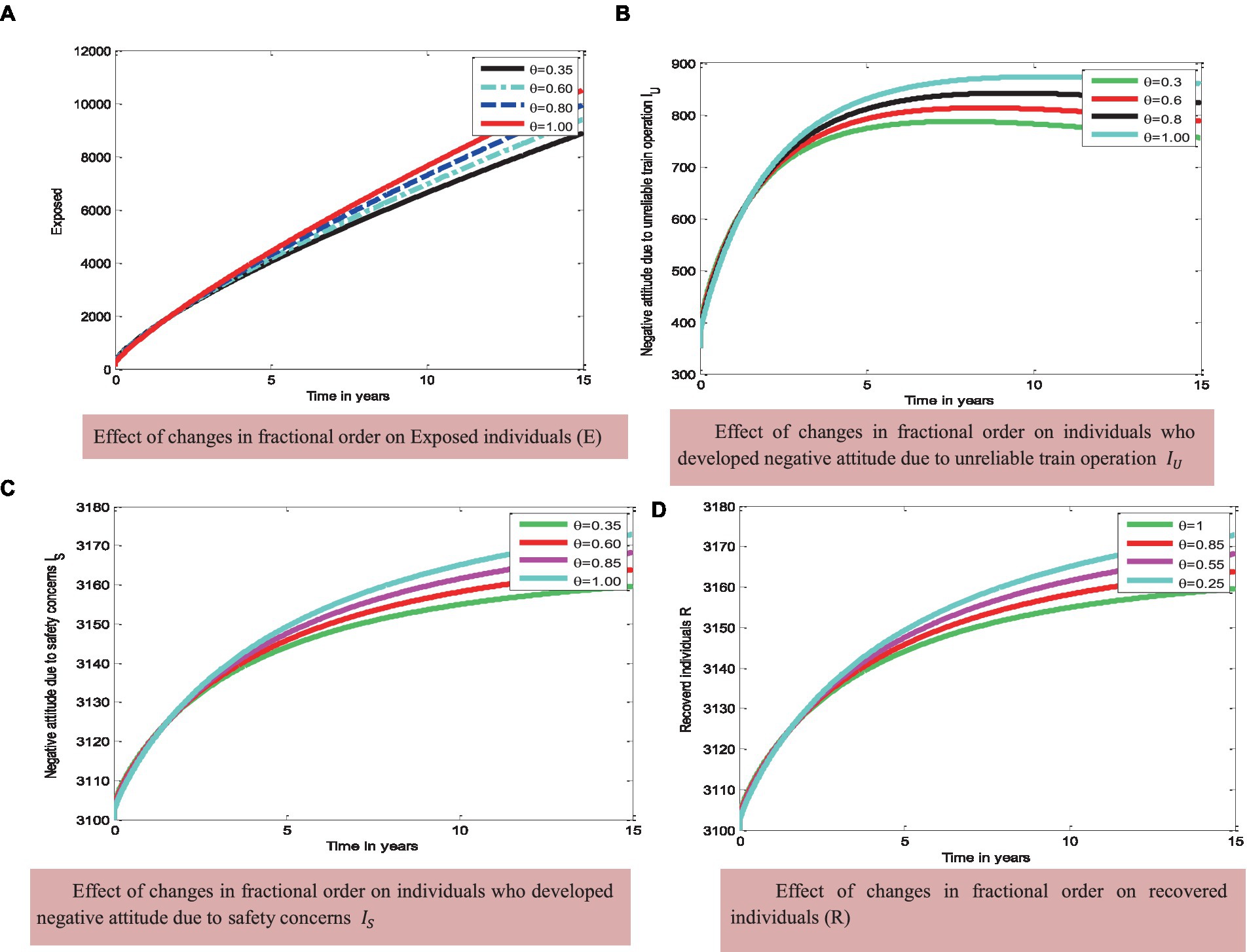
Figure 2. Effect of fractional order on the status of the state variables.

Moreover, decreasing fractional order leads to an increase in the number of passengers whose negative attitudes toward railway transportation have changed. This indicates that the fractional order model yields better model accuracy than the integer order model.

5.2 Numerical simulation of the optimal control problem

To assess the effects of controlling strategies and validate the analytical findings of the fractional order optimal control problem, we conducted a numerical simulation (Equation 13) using MATLAB 2023a programming codes.

We employed the Euler forward or/and backward finite difference method for the simulation, using different initial conditions and assuming specific baseline parameter values to be ${\chi }_1={\chi }_2={\chi }_3=32$ , ${\Gamma }_1=40$ , ${\Gamma }_2=43$ , ${\Gamma }_3=48,$ $q=0.5$ , $\beta =0.38$ , $\eta =0.34$ , $\mathrm{\hspace{0.33em}}{\mathrm{d}}_2=0.2$ , $d=0.23,$ $\mathrm{K}=100$ , $\mathrm{\hspace{0.33em}}\varpi =0.4$ , $\mathrm{\hspace{0.33em}}{\alpha }_1=0.45\mathrm{\hspace{0.33em}}$ , and ${\alpha }_2=0.38$ . In this subsection, we conducted a numerical simulation using the Euler forward method to investigate the impact of controlling strategies on the state variables in the optimal control problem (Equation 13). We assumed that the order of the derivative is $\vartheta =0.96$ .

Figures 3–5 in the numerical simulations demonstrated the importance of control strategies in addressing the dissemination of negative attitudes among passengers in the community. We considered optimal controlling strategies to showcase the impact of protection and improvement measures on reducing transmission rates. The first strategy involves implementing only the protection strategy ( $u_1$ ). The second strategy focuses solely on the improvement of the attitudes individuals ( $u_2$ ) who developed negative attitudes due to safety concerns. The third strategy targets the improvement of the attitudes of individuals ( $u_3)$ who developed negative attitudes due to unreliable train operation. The fourth strategy combines both improvement strategies ( $u_2$ and $u_3$ ) simultaneously, and finally, the fifth strategy involves implementing all of the controlling strategies ( $u_1$ , $u_2$ , and $u_3$ ) together.

Figure 3

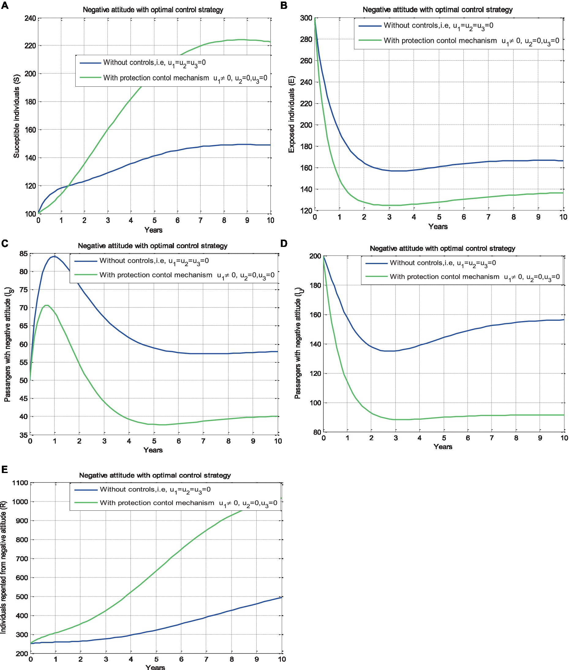
Figure 3. Effect of the prevention strategy (𝑢₁) on the negative attitude status of different population groups with 𝜗=0.96.

Figure 4

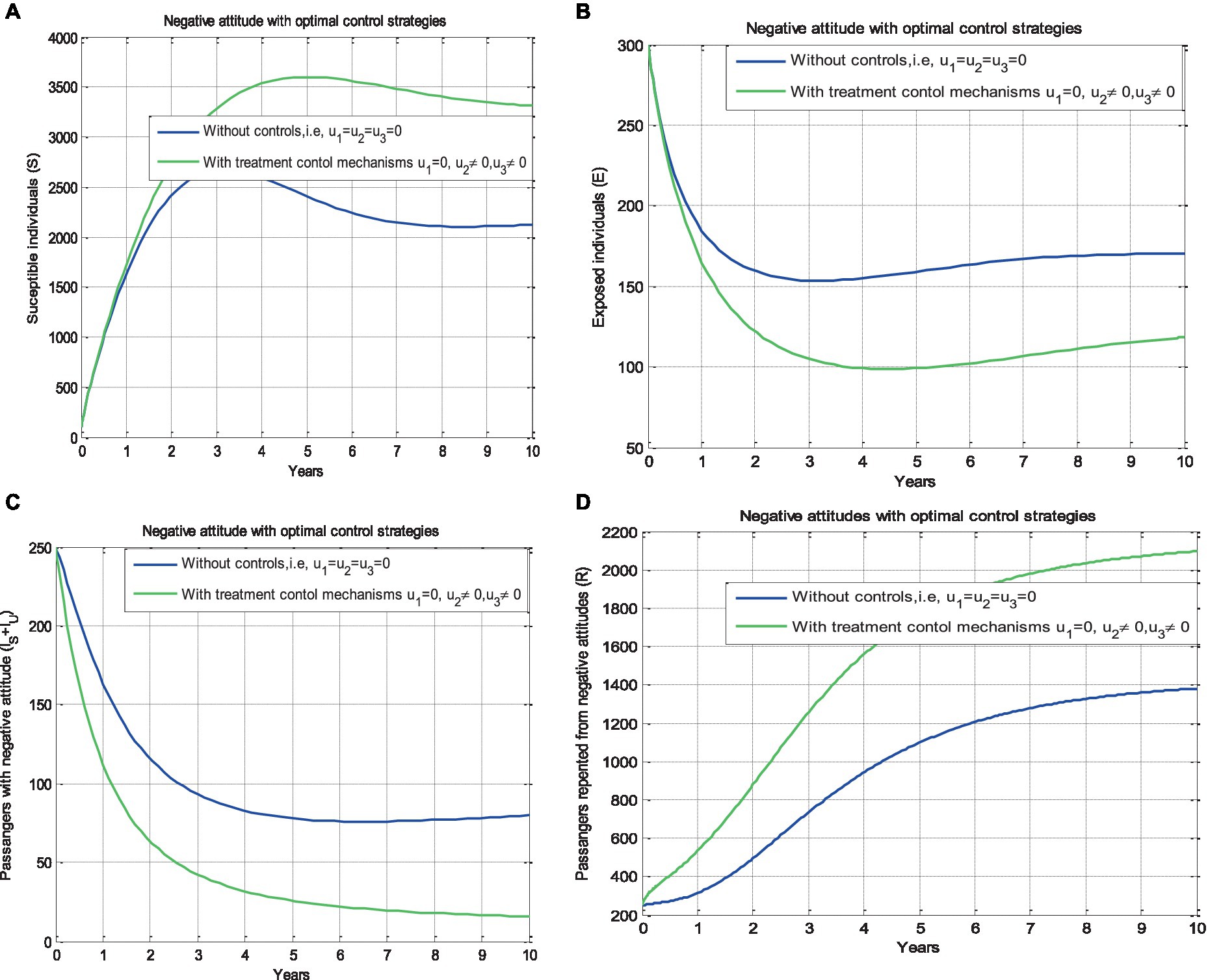
Figure 4. Effect of the improvement strategies [𝑢₂ and (𝑢₃)] on the negative attitude status of different population groups with 𝜗=0.96.

Figure 5

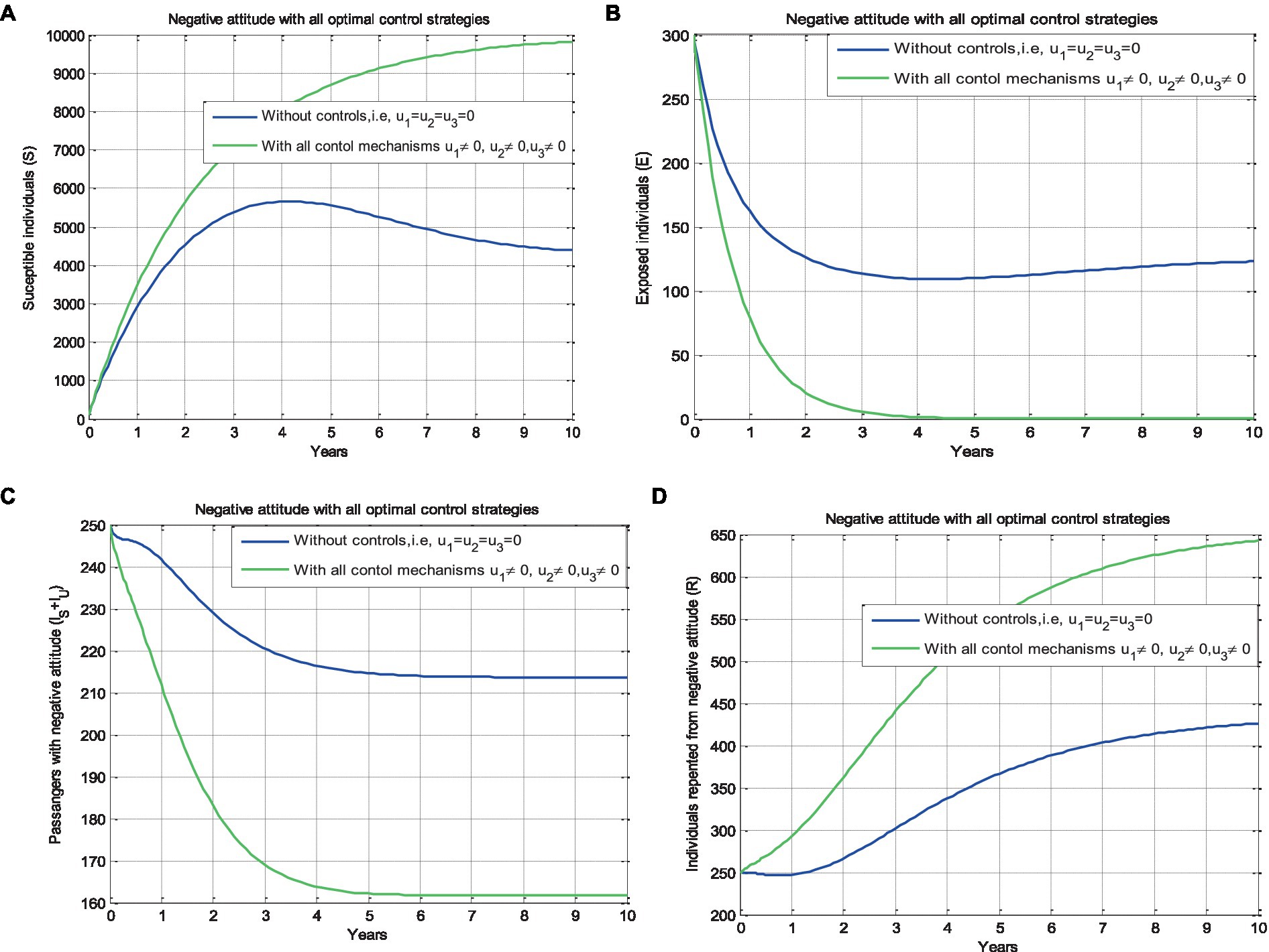
Figure 5. Effect of all the control strategies (𝑢₁ = 0 𝑢₂ = 0 and 𝑢₃= 0) simultaneously on the passengers’ negative attitude status of different population groups with 𝜗 = 0.96.

5.2.1 Effect of protection ( $u_1\ne 0$ )

In this sub-section, we conducted a numerical simulation under two conditions: one without applying improvement-controlling strategies and the other with the implementation of a preventive strategy (Strategy 1), that is, by setting $u_1\ne 0$ , $\mathrm{\hspace{0.33em}}{u}_2=0,$ and $u_3=0$ while also considering the value $\vartheta =0.96$ . The graphical representation in Figure 3 that illustrates the influence of the prevention strategy on the dynamics of passengers’ transmission of negative attitudes shows that implementing the controlling strategy $u_1$ significantly decreases the exposed passengers, the passengers who developed negative attitudes due to safety concerns, and the passengers who developed negative attitudes due to unreliable train operation, while there was an increase in the number of susceptible passengers and in the number of passengers whose negative attitudes changed.

5.2.2 Effect of improvement strategies ( $u_2\ne 0\mathrm{\hspace{0.33em}}$and $\mathrm{\hspace{0.33em}}{u}_3\ne 0$ )

In this subsection, we performed numerical simulations without applying a protection control strategy $(u_1$ ) and applying the improvement strategies $\mathrm{\hspace{0.33em}}(u_2\ne 0\mathrm{\hspace{0.33em}}a$nd $\mathrm{\hspace{0.33em}}{u}_3\ne 0)$ . From the simulation illustrated by Figure 4B shows that individuals in the exposed class are reduced slightly as compared to Figure 3B, but passengers who developed negative attitudes due to safety concerns and the passengers who developed negative attitudes due to unreliable train operation are reduced rapidly compared to the first similar classes.

5.2.3 Effect of protection and improvement strategies ( $u_1\ne 0,u_2\ne 0,$and $\mathrm{\hspace{0.33em}}{u}_3\ne 0)$

In this subsection, we performed numerical simulations without applying all controlling strategies in place and by applying all possible controlling strategies $(u_1\ne 0,u_2\ne 0,$and $\mathrm{\hspace{0.33em}}{u}_3\ne 0)$ simultaneously.

Here, we can compare the impact of implementing the different control strategies on the emergence of negative attitudes. Figure 5A demonstrates that implementing all proposed control strategies significantly increases the number of susceptible individuals compared to the numbers shown in Figures 3A, 4A. Additionally, Figure 5B illustrates that all proposed controlling strategies greatly decrease the number of exposed individuals compared to the number of exposed individuals illustrated in Figures 3B, 4B. Furthermore, Figure 5C reveals that all proposed controlling strategies have a considerable impact on reducing the number of passengers who developed negative attitudes compared to the numbers in Figures 3C,D, 4C. Finally, in Figure 5D, implementing all proposed strategies notably increases the number of individuals whose negative attitudes changed compared to the number of individuals whose negative attitudes changed as illustrated in Figures 3E, 4D. Ultimately, it is observed from Figure 5 that applying all possible controlling strategies $(u_1\ne 0,u_2\ne 0,$ and $\mathrm{\hspace{0.33em}}{u}_3\ne 0)$ simultaneously leads to a significant reduction in the number of passengers who develop negative attitudes in the community after 10 years. When compared to other strategies, implementing protection alone or improvement strategies alone, both protection and improvement strategies together is the most effective strategy in addressing the evolution of negative attitudes due to unreliable train operations or safety concerns among passengers in the community.

6 Conclusion

In this study, the dynamics of passengers who developed negative attitudes by applying the Caputo fractional order derivative approach whenever the fractional order $\vartheta =0.96$ is presented. Some fundamental proprieties of the solutions of the proposed fractional order model, such as existence, uniqueness, positivity, and boundedness, are analyzed. We derived the formula for the model’s basic reproduction number using the next-generation operator approach. Using the stability criteria for the fractional order model, we analyzed the results of the stability of the proposed model with respect to the basic reproduction number. We examined the local and global asymptotical stability of the negative attitude-free equilibrium points whenever the corresponding basic reproduction number is less than unity.

Moreover, we carried out the local and global stability of the negative attitude endemic equilibrium point of the model. We formulated and analyzed the corresponding optimal control problem for the fractional order model by incorporating three time-dependent control strategies: prevention measures, improvement measures for negative attitudes due to safety concerns, and improvement measures for negative attitudes due to unreliable train operation by applying the Pontryagin’s maximum principle. Moreover, using the well-known Euler’s forward or/and backward finite difference numerical methods, we established the results of the numerical simulation of the proposed optimal control problem. From the results of the numerical simulation given in Figure 5, we concluded that applying all possible controlling strategies $(u_1\ne 0,u_2\ne 0,$and $\mathrm{\hspace{0.33em}}{u}_3\ne 0)$ simultaneously greatly decreases the number of passengers who developed negative attitudes in the community after a decade. Strategy 4 is the most effective strategy to tackle the disseminating rate of passengers’ negative attitudes throughout the community compared to other strategies.

Finally, as this study is not comprehensive, other researchers in the field have the opportunity to enhance the proposed model by including additional factors such as a stochastic approach, considering the age structure of passengers and refining the model with relevant real-world data.

Data availability statement

The original contributions presented in the study are included in the article/Supplementary material, further inquiries can be directed to the corresponding author.

Author contributions

GH: Conceptualization, Formal analysis, Investigation, Methodology, Resources, Software, Supervision, Validation, Visualization, Writing – original draft, Writing – review & editing. ST: Conceptualization, Formal analysis, Investigation, Methodology, Resources, Software, Supervision, Validation, Visualization, Writing – original draft, Writing – review & editing.

Funding

The author(s) declare that no financial support was received for the research, authorship, and/or publication of this article.

Conflict of interest

The authors declare that the research was conducted in the absence of any commercial or financial relationships that could be construed as a potential conflict of interest.

Publisher’s note

All claims expressed in this article are solely those of the authors and do not necessarily represent those of their affiliated organizations, or those of the publisher, the editors and the reviewers. Any product that may be evaluated in this article, or claim that may be made by its manufacturer, is not guaranteed or endorsed by the publisher.

Supplementary material

The Supplementary material for this article can be found online at: https://www.frontiersin.org/articles/10.3389/fams.2024.1290494/full#supplementary-material

References

1. Alemu, A. Success factors and challenges of railway megaprojects in Ethiopia. J Bus Adm Stud (2016) 8:1.

Google Scholar

2. Berger, A, Hoffmann, R, Lorenz, U, and Stiller, S. Online railway delay management: hardness, simulation and computation. Simulation (2011) 87:616–29. doi: 10.1177/0037549710373571

Crossref Full Text | Google Scholar

3. Dziekan, K. (2008). Ease-of-use in Public Transportation: A User Perspective on Information and Orientation Aspects. Stockholm, Sweden: Royal Institute of Technology.

Google Scholar

4. Cheng, YH. Exploring passenger anxiety associated with train travel. Transportation (2010) 37:875–96. doi: 10.1007/s11116-010-9267-z

Crossref Full Text | Google Scholar

5. Currie, G, and Muir, C. Understanding passenger perceptions and behaviors during unplanned rail disruptions. Transp Res Procedia (2017) 25:4392–402. doi: 10.1016/j.trpro.2017.05.322

Crossref Full Text | Google Scholar

6. Marteache, N, Bichler, G, and Enriquez, J. Mind the gap: perceptions of passenger aggression and train car supervision in a commuter rail system. J Public Transp (2015) 18:61–73. doi: 10.5038/2375-0901.18.2.5

Crossref Full Text | Google Scholar

7. Kuo, T, Chen, CT, and Cheng, WJ. Service quality evaluation: moderating influences of first-time and revisiting customers. Total Qual Manag Bus Excell (2018) 29:429–40. doi: 10.1080/14783363.2016.1209405

Crossref Full Text | Google Scholar

8. Din, A, Khan, FM, Khan, ZU, Yusuf, A, and Munir, T. The mathematical study of climate change model under nonlocal fractional derivative. Partial Differ Equ Appl Math (2022) 5:100204. doi: 10.1016/j.padiff.2021.100204

Crossref Full Text | Google Scholar

9. Sene, N. Analytical solutions of a class of fluids models with the Caputo fractional derivative. Fractal Fract (2022) 6, 3–8. doi: 10.3390/fractalfract6010035

Crossref Full Text | Google Scholar

10. Ghosh, U, Pal, S, and Banerjee, M. Memory effect on Bazykin’s prey-predator model: stability and bifurcation analysis. Chaos, Solitons Fractals (2021) 143, 3–14. doi: 10.1016/j.chaos.2020.110531

Crossref Full Text | Google Scholar

11. de Barros, LC, Lopes, MM, Pedro, FS, Esmi, E, dos Santos, JPC, and Sánchez, DE. The memory effect on fractional calculus: an application in the spread of COVID-19. Comput Appl Math (2021) 40:4–5. doi: 10.1007/s40314-021-01456-z

Crossref Full Text | Google Scholar

12. Podlubny, I. Fractional Differential Equations: An Introduction to Fractional Derivatives, Fractional Differential Equations, to Methods of Their Solution and Some of Their Applications, vol. 198. San Diego, California, USA: Academic Press. (1999).

Google Scholar

13. Mandal, M, Jana, S, Nandi, SK, and Kar, TK. Modelling and control of a fractional-order epidemic model with fear effect. Energy Ecol Environ (2020) 5:421–32. doi: 10.1007/s40974-020-00192-0

PubMed Abstract | Crossref Full Text | Google Scholar

14. Matignon, D. Stability results for fractional differential equations with applications to control processing. Comput Eng Syst Appl (1996).

Google Scholar

15. Teklu, SW. Analysis of fractional order model on higher institution students’ anxiety towards mathematics with optimal control theory. Sci Rep (2023) 13:6867. doi: 10.1038/s41598-023-33961-y

PubMed Abstract | Crossref Full Text | Google Scholar

16. Ahmed, E, El-Sayed, AMA, and El-Saka, HAA. On some Routh-Hurwitz conditions for fractional order differential equations and their applications in Lorenz, Rössler, Chua and Chen systems. Phys Lett Sect A Gen At Solid State Phys (2006) 358:1–4. doi: 10.1016/j.physleta.2006.04.087

Crossref Full Text | Google Scholar

17. Vargas-De-León, C. Volterra-type Lyapunov functions for fractional-order epidemic systems. Commun Nonlinear Sci Numer Simul (2015) 24:75–85. doi: 10.1016/j.cnsns.2014.12.013

Crossref Full Text | Google Scholar

18. Bhalekar, S, and Patil, M. Singular points in the solution trajectories of fractional order dynamical systems. Chaos (2018) 28:113123. doi: 10.1063/1.5054630

PubMed Abstract | Crossref Full Text | Google Scholar

19. Echenausía-Monroy, JL, Gilardi-Velázquez, HE, Jaimes-Reátegui, R, Aboites, V, and Huerta-Cuellar, G. A physical interpretation of fractional-order-derivatives in a jerk system: electronic approach. Commun Nonlinear Sci Numer Simul (2020) 90:105413. doi: 10.1016/j.cnsns.2020.105413

Crossref Full Text | Google Scholar

20. Zhou, P, Ma, J, and Tang, J. Clarify the physical process for fractional dynamical systems. Nonlinear Dyn (2020) 100:2353–64. doi: 10.1007/s11071-020-05637-z

Crossref Full Text | Google Scholar

21. Petrás, I. (2011). Fractional-Order Nonlinear Systems. Modeling, Analysis and Simulation. Springer, Berlin, Heidelberg. doi: 10.1007/978-3-642-18101-6_2

Crossref Full Text | Google Scholar

22. Mainardi, F. Why the mittag-leffler function can be considered the queen function of the fractional calculus? Entropy (2020) 22, 2–3. doi: 10.3390/e22121359

PubMed Abstract | Crossref Full Text | Google Scholar

23. Fernandez, A, and Husain, I. Modified mittag-leffler functions with applications in complex formulae for fractional calculus. Fractal Fract (2020) 4:1–2. doi: 10.3390/fractalfract4030045

Crossref Full Text | Google Scholar

24. Özarslan, MA, and Fernandez, A. On the fractional calculus of multivariate Mittag-Leffler functions. Int J Comput Math (2022) 99:247–73. doi: 10.1080/00207160.2021.1906869

Crossref Full Text | Google Scholar

25. Balatif, O, Boujallal, L, Labzai, A, and Rachik, M. Stability analysis of a fractional-order model for abstinence behavior of registration on the electoral lists. Int J Differ Equa (2020) 2020:1–8. doi: 10.1155/2020/4325640

Crossref Full Text | Google Scholar

26. Teklu, SW, and Terefe, BB. Mathematical modeling analysis on the dynamics of university students animosity towards mathematics with optimal control theory. Sci Rep (2022a) 12:11578. doi: 10.1038/s41598-022-15376-3

PubMed Abstract | Crossref Full Text | Google Scholar

27. Teklu, SW, and Terefe, BB. Mathematical modeling investigation of violence and racism coexistence as a contagious disease dynamics in a community. Comput Math Methods Med (2022b) 2022:1–13. doi: 10.1155/2022/7192795

PubMed Abstract | Crossref Full Text | Google Scholar

28. Pontryagin, LS, Boltyanskii, VG, Gamkrelidze, RV, Mishchenko, EF, Trirogoff, KN, and Neustadt, LW. L. S. Pontryagin selected works: the mathematical theory of optimal processes. Angew Chem Int Ed (1967) 6:951–2.

Google Scholar

29. Yang, WY, Cao, W, Chung, TS, and Morris, J. Applied Numerical Methods Using MATLAB®, Hoboken, New Jersey: John Wiley and Sons (2005).

Google Scholar