 Isaac Mwangi Wangari
 Samson Olaniyi
 Ramoshweu S. Lebelo
 Kazeem O. Okosun4
94% of researchers rate our articles as excellent or good
Learn more about the work of our research integrity team to safeguard the quality of each article we publish.
Find out more
ORIGINAL RESEARCH article
Front. Appl. Math. Stat., 07 December 2023
Sec. Mathematical Biology
Volume 9 - 2023 | https://doi.org/10.3389/fams.2023.1292443
This article is part of the Research TopicModelling and Numerical Simulations with Differential Equations in Mathematical Biology, Medicine and the Environment: Volume IIView all 6 articles
Introduction: The unexpected emergence of novel coronavirus identified as SAR-CoV-2 virus (severe acute respiratory syndrome corona virus 2) disrupted the world order to an extent that the human activities that are core to survival came almost to a halt. The COVID-19 pandemic created an insurmountable global health crisis that led to a united front among all nations to research on effective pharmaceutical measures that could stop COVID-19 proliferation. Consequently, different types of vaccines were discovered (single-dose and double-dose vaccines). However, the speed at which these vaccines were developed and approved to be administered created other challenges (vaccine skepticism and hesitancy).
Method: This paper therefore tracks the transmission dynamics of COVID-19 using a non-linear deterministic system that accounts for the unwillingness of both susceptible and partially vaccinated individuals to receive either single-dose or double-dose vaccines (vaccine hesitancy). Further the model is extended to incorporate three time-dependent non-pharmaceutical and pharmaceutical intervention controls, namely preventive control, control associated with screening-management of both truly asymptomatic and symptomatic infectious individuals and control associated with vaccination of susceptible individuals with a single dose vaccine. The Pontryagin's Maximum Principle is applied to establish the optimality conditions associated with the optimal controls.
Results: If COVID-19 vaccines administered are imperfect and transient then there exist a parameter space where backward bifurcation occurs. Time profile projections depict that in a setting where vaccine hesitancy is present, administering single dose vaccines leads to a significant reduction of COVID-19 prevalence than when double dose vaccines are administered. Comparison of the impact of vaccine hesitancy against either single dose or double dose on COVID-19 prevalence reveals that vaccine hesitancy against single dose is more detrimental than vaccine hesitancy against a double dose vaccine. Optimal analysis results reveal that non-pharmaceutical time-dependent control significantly flattens the COVID-19 epidemic curve when compared with pharmaceutical controls. Cost-effectiveness assessment suggest that non-pharmaceutical control is the most cost-effective COVID-19 mitigation strategy that should be implemented in a setting where resources are limited.
Discussion: Policy makers and medical practitioners should assess the level of COVID-19 vaccine hesitancy inorder to decide on the type of vaccine (single-dose or double-dose) to administer to the population.
The advent of COVID-19 infection whose aetiological agent is SARS-CoV-2 virus (severe acute respiratory syndrome corona virus 2) caught the world off guard. The index case of COVID-19 was first confirmed in Wuhan city, Hubei province in China as early as December 2019. Within a period of about 60 days, COVID-19 spread from the epicenter (Wuhan city) to other countries in the world, leading to WHO declaring COVID-19 a global pandemic on March 2020 [1, 2]. The main routes of COVID-19 transmission are direct spread, contact spread, and aerosol spread [3]. Direct spread of COVID-19 occurs as a result of exhaling respiratory droplets from sneezing or coughing. Individuals who are in close contact with other individuals who are suspected or confirmed being infected with COVID-19 can as well be infected [4, 5]. As for the indirect transmission, it may occur when individuals touch eyes, nose, or mouth after contacting contaminated surfaces or objects [4, 5]. Infected individuals are broadly categorized as either asymptomatic (which include both pre-symptomatic and true asymptomatic) or symptomatic. Symptomatic individuals manifest various symptoms which include viral pneumonia, dry cough, fever, myalgia, sore throat, fatigue, nasal congestion, and diarrhea [6, 7]. There is concrete evidence in the sequel that shows that pre-symptomatic transmission significantly contributes to the spread of COVID-19 [8]. Although the field of corona virology was well documented in the sequel [9], the interaction of corona viruses strains with human population on a global scale was not witnessed before. Even when there was SARS outbreak between 2002 and 2003 in North America, South America, Europe, and Asia, it caused about 8,098 cases and 774 SARS-induced fatalities [9] which was significantly low in comparison with 524,467,084 COVID-19-confirmed cases and over 6,915,286 (and increasing) COVID-19-related deaths reported globally [10].
The rapid speed at which COVID-19 established itself within communities triggered myriad challenges such as disruption of normal life, loss of source of livelihood, shrinking of economies (in particular in developing countries), and insurmountable straining of the existing health infrastructure [11]. Exponential increase of critically ill patients in need of urgent medical attention particularly requiring ventilators created a burden within the health system that has never been witnessed in the 21st century. Governments across the world implemented stringent countermeasures to halt the spread of the COVID-19 pandemic. Initially, these suppressive intervention measures were non-pharmaceutical in nature, and they included lock down, contact tracing and quarantine, a ban on air traffic, social distancing, wearing face masks and washing hands regularly, suspending traveling in and out of countries, banning all social gatherings, closing schools, airing awareness programs, and PCR testing for case detection [5, 12]. However, these non-pharmaceutical interventions (NPIs) were short-term measures against proliferation of COVID-19 [13]. A sudden rebound of COVID-19 spread occurred once these intervention measures were relaxed [14]. Consequently, there was a global consensus that pharmaceutical measures such as development of COVID-19 vaccines and cure could mitigate the spread of COVID-19 pandemic.
The proliferation of COVID-19 pandemic compelled multilateral global organizations and private funders to collectively raise funds for researching on an effective vaccine against the novel SARS-CoV-2 [15]. On 11 January 2020, the genetic sequence of SARS-CoV-2 (the causative agent of COVID-19) was made public [16]. Following this breakthrough, the Coalition for Epidemic Preparedness Innovation (CEPI) tasked the global pharmaceutical companies and virology research institutes to conduct a cutting edge research on COVID-19 vaccines. Within a period of about 4 months after emergence of COVID-19, there were about 115 COVID-19 vaccine candidates that were either at exploratory or pre-clinical stages [16]. Shortly afterward, some of these vaccines in particular mRNA-1273 from Moderna, Ad5-nCoV from CanSino Biologicals, INO-4800 from Inovio, and LV-SMENP-DC and pathogen-specific aAPC from Shenzhen Geno-Immune Medical Institute moved into clinical development, and some developed countries started administering them to the general populace [16]. By early 2021, WHO and Food and Drug Administration (FDA) approved more COVID-19 vaccines such as AstraZeneca, Johnson and Johnson, and Pfizer, for the management of COVID-19 pandemic.
It is imperative to note that most of these vaccine innovation breakthroughs and manufacturing were initially based in developed countries. Given most of these high-income countries (HICs) were experiencing an exponential increase of COVID-19 cases on a daily basis, they implemented vaccine nationalism. According to Riaz et al. [15], vaccine nationalism is referred to as an economic strategy that involve hoarding vaccines from manufacturers so that the respective countries can have enough vaccines to vaccinate a large proportion of their populace without being concerned with the limited vaccine production and distribution for the rest of the world. Vaccine nationalism is well known to cause devastating consequences on affected countries. These include leaving many disadvantaged countries with low economic status unable to pay for vaccines as prices of vaccines hike over time; it decreases the likelihood of developing countries to access vaccines as they are likely to be out of stock even when they accumulate enough resources to buy them. Moreover, vaccine nationalism prolongs the duration of the pandemic as it will continue spreading within developing countries unabated [15]. One of the key factors that underpinned vaccine nationalism was that many pharmaceutical companies in various countries were competing in vaccine production. However, the competition was not for the sole purpose of supplying the vaccine to the “ailing humanity” at a subsidized rate but with the aim of selling the vaccines to countries which could offer “strong financial stock upholds” [17]. This policy made it harder for the low- and middle-income countries (LMICs) to afford vaccines, hence alienating them from the global target of vaccination against the lethal SARS-CoV-2. Nevertheless, these pharmaceuticals failed to recognize that the circulation of COVID-19 in developing countries still posed a potential threat to HICs as the cross-border traffic exacerbated COVID-19 transmission. Moreover, many COVID-19 experts in HICs argued that vaccinating some countries while neglecting others burdened with COVID-19 created a huge gap in attaining global immunity [18]. Furthermore, a surge in the population of infected individuals could render an advantageous environment for the mutations of the novel corona virus [19]. Hence, vaccine nationalism was regarded as a self-defeating policy [15].
WHO criticized vaccine nationalism and called for a global funding to increase vaccine production at unprecedented speed. In addition, WHO stressed on the importance of equitable distribution of vaccines among the nations (i.e., both HICs and LMICs) at a subsidized rate. This was in agreement with WHO's slogan that “no one is safe until everyone is safe” [20–23]. WHO vaccine equity sensitization suggested that equitable roll-out of COVID-19 vaccine will not only speed up the end of the pandemic but will considerably increase population immunity worldwide, relieve burdening of health systems, and facilitate rapid recovery of economies and reduction of the likelihood of new variants emerging [24]. By September 2021, COVID-19 vaccines were widely accessible by both HICs and LMICs. However, even with vaccines being available in both HICs and LMICs, other pertinent issues adversely impacted vaccine roll-out within the countries populace. Some of the fundamental issues being inequality in vaccine distribution, vaccine prioritization, and skepticism among different groups. Limited production of COVID-19 vaccines led to many countries providing vaccines to the most vulnerable cohorts. For instance, WHO, United Kingdom, and the United States prioritized offering vaccines to healthcare personnel, individuals with high risk of developing severe symptoms that can lead to death, the elderly, and individuals with co-morbidities [13, 25, 26]. Vaccine distribution inequality was also observed even within a particular cohort (e.g., among health care workers). Studies by Chen and Krieger [27] Ogedegbe et al. [28] and Vahidy et al. [29] signaled that there is considerable inequalities in COVID-19 burden in terms of race, ethnicity, and socio-economic status which is impacted by distribution and prioritization of vaccinations. They suggested that barriers that hinder vaccine distribution should be identified and removed [30]. Although there is gradual reduction of vaccine distribution inequality, the number of individuals vaccinated in developed countries is 69 times higher than in developing countries [22].
In addition to COVID-19 vaccine being attributed to COVID-19 reduction, individual willingness to receive COVID-19 jab significantly influenced vaccine distribution [15]. Although the desire to receive COVID-19 vaccine remains relatively high globally, obstacles such as vaccine skepticism and hesitancy hamper efforts to curb COVID-19 pandemic [31]. Vaccine skepticism is based on several factors. Some individuals refuse to be vaccinated as a result of vaccine safety concerns, especially the conviction that the vaccine is dangerous due to the speed at which it was produced [15]. Other individuals argued that the COVID-19 was harmless, and therefore, they did not see the need of receiving COVID-19 vaccine. Factors such as doubt of COVID-19 vaccine effectiveness, belief in pre-existing immunity, and the origin of the vaccine also contributed in vaccine skepticism [15, 31]. Some individuals reasoned that the long-term impact of COVID-19 vaccines was unknown and therefore refused to be vaccinated. Moreover, political reasons and conspiracy theories found in many social media fuelled vaccine hesitancy [32]. Factors such as detrimental impact of COVID-19 on the lives of milliards of people around the globe and devastation of the world economy were thought to be determinants that will fuel ubiquitous acceptance of COVID-19 vaccine [33]. However, this was not the case as suggested by many findings. The study by Neumann-Bohme and co-workers [34] assessed the level of anti-COVID-19 vaccination among citizens on seven European countries and found that hesitancy and resistance against the vaccines were substantial across all cohorts, age groups, and sexes. For instance, 38% of those interviewed in France were hesitant toward COVID-19 vaccine where 10% were opposed to COVID-19 vaccination while the remaining 28% were undecided about getting COVID-19 vaccination [33]. In the United States (US), a report by the American Medical Association Journal hinted that skepticism toward vaccines that were being administered was on the rise [35]. This was further corroborated by the Kaiser Family Foundation COVID-19 vaccine monitoring which indicated that approximately 29% of health practitioners were reluctant to accept the vaccine [36].
During the early onset of COVID-19 (i.e., before accumulation of enough data to predict and project on COVID-19 prevalence), COVID-19 mathematical models proved to be an invaluable tool (and they still are) on providing insights on the appropriate mitigation strategy to adopt to prevent COVID-19 spiraling. Many models that were formulated focused on elucidating how NPIs will impact COVID-19 transmission dynamics. For instance, COVID-19 models by Ngonghala et al. [37], Srivastav et al. [88], and Wangari et al. [38] showed that correct use of face masks by public is always beneficial. However, the studies emphasized that the beneficial impact of face masks coverage at population-level is linearly dependent on face mask efficacy. Furthermore, their results showed that if the public combined both face masks and physical/social distancing, then a significant decline in COVID-19 burden occurred. The article by Tiwari et al. [39] analyzed whether disseminating COVID-19 awareness at individual, community, and global level can influence general populace viewpoint and behavior toward COVID-19. Their findings showed that higher dissemination of COVID-19 awareness among susceptible population (in particular mouth-to mouth awareness dissemination) played a key role in preventing COVID-19 spread. Moreover, an increase in awareness rate led to a significant decline of asymptomatic individuals as well as number of symptomatic individuals requiring hospitalization. A closely related study by Rai et al. [40] assessed the effectiveness of social media advertisements in suppressing rates of interaction between susceptible individuals and COVID-19 infectious individuals in India. Their results showed that airing COVID-19 information through social media platform could play a vital role in suppressing COVID-19 transmission and therefore advocated such approach to be included as a mitigation strategy. Given the study conducted by Tiwari et al. [39] was done during early development of COVID-19 when there was insufficient information on COVID-19 epidemiological dynamics, their study did not capture the role pre-symptomatic infectious individuals could have played as far as COVID-19 prevalence was concerned. Moreover, the study by Tiwari et al. [39] did not include vaccination and vaccine hesitancy, perhaps due to the reason that vaccines were in their early clinical trial stage. Similarly, the article Rai et al. [40] did not consider a scenario where pre-symptomatic infectious individuals could contribute in COVID-19 transmission and also neglected vaccination as an intervention strategy, and therefore, they could not analyze impact of vaccine hesitancy in the general populace.
Shortly after WHO and Center for Disease Control (CDC) declared availability of COVID-19 vaccines, several epidemiological mathematical frameworks began to emerge with the aim of investigating whether vaccines will slow or end the COVID-19 pandemic as well as determining strategies that ensured optimal distribution of COVID-19 vaccines [41–44]. In the sequel, few epidemiological mathematical models have attempted to elucidate on the impact vaccine hesitancy played in the early roll-out of COVID-19 vaccines [33, 35]. Some pertinent questions that relate to vaccine hesitancy have been investigated as far as COVID-19 vaccine roll-out is concerned. For example, authors in Oduro et al. [35] proposed a model that stratified the general populace depending on their willingness and unwillingness to receive COVID-19 jab. Their study exclusively investigated how educating the unwilling population about the importance of COVID-19 vaccine will impact COVID-19 transmission dynamics. Their findings suggested that education of the unwilling individuals such that they accept to get COVID-19 vaccines led to a significant reduction of control reproduction number. Although their study mentioned about vaccine hesitancy as the motivation behind incorporating education parameter among unwilling cohorts, their study did not incorporate parameters that explicitly modeled vaccine hesitancy. Moreover, vaccine hesitancy may occur in several stages especially in a scenario where COVID-19 vaccine are offered at certain intervals. For example, some vaccines such as AstraZeneca required individuals to get two doses of vaccines before one is considered to be fully vaccinated. In some cases, some individuals refused to get second dose of vaccine with the justification that they experienced severe side effects. The study by Oduro et al. [35] never captured vaccine hesitancy among partially vaccinated individuals. Buonomo et al. [33] considered a behavioral epidemiology approach to model how vaccination campaign impacted COVID-19 dynamics. The study incorporated vaccination rate as a function of the present and past information that the general populace have on the spread of the COVID-19 pandemic. Their approach was similar to the one used by dOnofrio and Manfredi [45] where they showed that incorporation of information-related changes in contact patterns induces oscillations in the endemic prevalence of infectious diseases. Similarly, the study by Buonomo et al. [33] did not consider a possibility where vaccine hesitancy could occur among different cohorts, given vaccines are also administered in phases (first dose, second dose and booster shots).
The recent study by Peter et al. [46] proposed a mathematical model that incorporated a double-dose vaccination strategy. In their study Peter et al. [46], they assumed that vaccine is administered in two phases (first dose followed by the second dose). One major assumption in their study was that fully vaccinated individuals acquired a complete vaccine-induced immunity, and therefore, these individuals could neither experience breakthrough infections nor waning of the vaccine-induced immunity. Moreover, vaccine hesitancy was not accounted for in their model. Furthermore, despite mentioning that pre-symptomatic individuals greatly contribute in the spread of COVID-19, their force of infection did not explicitly capture transmission by pre-symptomatic individuals. A single-dose vaccination strategy was not considered in Peter et al. [46], despite existence of a concrete evidence that some vaccines require individuals to receive a single dose to be considered fully vaccinated against COVID-19 [47]. For example, Johnson & Johnson COVID-19 vaccine required individuals to receive a single dose. Scientific evidence demonstrated that Johnson & Johnson vaccine rendered 85% effectiveness in preventing individuals from developing severe COVID-19 symptoms that led to COVID-19-related hospitalizations and mortality [47]. Kumar et al. [48] have recently investigated how contamination of environment and surfaces with COVID-19 could influence COVID-19 transmission dynamics in the presence of vaccination. Although the study [48] incorporated vaccination (as a mitigation strategy) without distinguishing between a single-dose or double-dose vaccine, they did not consider the epidemiological implication of vaccine hesitancy as far as COVID-19 pandemic is concerned.
The novelty of this study stems from first recognizing that pre-symptomatic infectious individuals contribute significantly in the spread of COVID-19 [8], and therefore, the impact on how pre-symptomatic individuals affect COVID-19 transmission dynamics needs to be closely examined. Second, our study is the first to consider a scenario where vaccine hesitancy is assumed to occur in two phases depending on individual's choice of vaccine type (single dose or double dose), that is, first phase of vaccine hesitancy is assumed to occur among all susceptible individuals regardless of the choice of vaccine type. The second phase of vaccine hesitancy is only assumed to occur among individuals who choose double-dose vaccine. We will, therefore, investigate epidemiological implication likely to be witnessed if individuals who choose double-dose vaccine refuse second dose and therefore remain partially vaccinated. Noteworthy partially vaccinated individuals potentially pose a greater risk to COVID-19 mitigation measures than fully vaccinated individuals [49, 50]. Moreover, this study comprehensively compares how vaccine hesitancy against either single dose or double dose influences COVID-19 transmission dynamics. To the best of our knowledge, this comparison was not done in previous studies [33, 35, 41–44, 46, 48]. Findings in this study could form the basis for policymakers and medical practitioners in deciding the type of vaccine (single dose or double dose) to administer to a given community if the levels of vaccine hesitancy are known to be either relatively low/high.
Thus, our present study recognizes the gaps and relax the assumptions made in the studies [33, 35, 41–44, 46]. Consequently, the study considers a scenario where both single-dose vaccine and a double-dose vaccination strategies are concurrently adopted. Both single- and double-dose vaccination strategies are assumed to be hindered by vaccine hesitancy in the general populace. In this study we aim to:
1. Investigate whether pre-symptomatic individuals played a significant role as far as COVID-19 transmission dynamics is concerned?
2. Determine which type of vaccine (single dose or double dose) is most suitable in a setting where vaccine hesitancy is relatively low/high?
3. Determine the most cost-effective COVID-19 mitigation strategy, especially in a scenario where both NPIs and pharmaceutical control measures are concurrently being advocated by policymakers and medical practitioners (this will be achieved by extending the proposed model using optimal control theory)?
In this section, a model framework that describes COVID-19 transmission dynamics in a population where vaccine is available is presented. We assume that the government has not implemented any policy that requires all individuals to be vaccinated against COVID-19, that is, vaccination is non-mandatory. Therefore, we will consider a scenario where some individuals who have received the first COVID-19 vaccine have a choice to refuse the second dose (remain partially vaccinated). Moreover, we have considered a possibility where some individuals receive a single-dose vaccine rather than a two phase vaccine (double dose vaccine). Hence, we shall assume that COVID-19 vaccines available in the population are administered at different phases. First, we introduce notations that are necessary for the classification of individuals in the population depending on their health status. At any time t, we let N denotes the total population. N is divided into eight mutually exclusive compartments:
1. Susceptible, S: individuals who are considered to be healthy and are liable to contract COVID-19,
2. Vaccinated, Vp: individuals who have received the first dose of COVID-19 vaccine and are assumed to be partially protected. Hence, they can be infected with COVID-19 although at a reduced rate in comparison with susceptible individuals,
3. Vaccinated, V: individuals who have received either double-dose COVID-19 vaccine or the single-dose vaccine and are therefore considered to be fully vaccinated against COVID-19, but they can experience breakthrough infections at a relatively lower rate compared to both partially vaccinated and susceptible individuals,
4. Exposed E: consists of individuals who have been exposed to SARS-CoV-2, but are not capable of passing the virus to other healthy individuals, reason being that the virus incubation period has not yet elapsed,
5. Pre-symptomatic, Ip: This cohort includes individuals who are at post-latency stage (i.e., individuals who are in the incubation phase following latency). They are asymptomatic and able to transmit SARS-CoV-2,
6. Asymptomatic infectious Ia: This cohort includes individuals who remain asymptomatic throughout the course of the infection, but are able to pass the SARS-CoV-2 to others. Often regarded as truly asymptomatic individuals,
7. Symptomatic infectious, Is: Include individuals who manifest either mild or severe COVID-19 symptoms and are able to spread SARS-CoV-2,
8. Recovered, R: This cohort includes those who have recovered after infectious period.
The size of each class at any given time t describes the state variable of the model framework and N = S + Vp + V + E + Ip + Ia + Is + R. For the proposed model framework, we shall assume both a double-dose vaccine and a single-dose vaccines are concurrently being administered, contrary to study [33] that considered a single-dose vaccine which rendered a lifelong protection against COVID-19. It is assumed that the vaccine-induced immunity is not perfect and can wane over time. Therefore, vaccine-induced immunity among individuals who are fully vaccinated against COVID-19 and individuals who have received one dose of COVID-19 vaccine can wane over time such that it is of the same level as susceptible individuals; hence, they are assumed to join S compartment. Regarding transmission of COVID-19 among susceptible, partially vaccinated and fully vaccinated individuals, we assume that infection occurs as a result of interaction with three infectious cohorts, namely, pre-symptomatic infectious individuals, truly asymptomatic infectious individuals, and symptomatic infectious individuals. Transmission of COVID-19 by pre-symptomatic individuals is based on the findings that individuals exposed to COVID-19 are most infectious during the post-latency stage when they are not manifesting COVID-19 symptoms (usually 1–2 days before symptoms set in) [2, 8]. Research on this finding is still ongoing. On the one hand, truly asymptomatic individuals transmit COVID-19 at a relatively low rate in comparison with pre-symptomatic individuals. This assumption corroborates well with the finding that truly asymptomatic patients cause little or no transmission of COVID-19 [51].
In the proposed COVID-19 model, the force of infection which represents the per capita rate at which susceptible, partially vaccinated individuals and fully vaccinated individuals contract COVID-19 is assumed to be a mass action incidence defined as λ = β(Ip + η1Ia + η2Is). The justification behind choosing a mass action incidence is a 2-fold. One being that during the COVID-19 pandemic, the total population remained relatively constant [33]. Second, mass action incidence is chosen for mathematical simplification and tractability. Note that in the force of infection, parameters η1 and η2 are modification coefficients that account for reduced infectiousness of truly asymptomatic and symptomatic individuals when compared with infectious post-latency individuals (pre-symptomatic individuals). Parameter β represents the effective contact rate. All subgroups decrease due to natural mortality at per capita rate μ per day, while infectious symptomatic individuals experience an extra mortality due to COVID-19-induced death at per capita rate d per day.
Recruitment into susceptible subgroup S occurs at a rate ∧ humans per day. Since first dose vaccine-induced immunity is not lifelong (imperfect to protect against COVID-19), partially vaccinated individual immunity can wane at a rate ω1 per day and these individuals revert to susceptible class. Similarly, fully vaccinated individual immunity can wane over time, and these individuals return to susceptible subgroup at a rate ω2 per day. Due to myriad challenges that faced COVID-19 vaccine distribution during the early days, among them being vaccine hesitancy (just to mention a few) the rates at which susceptible individuals in the class S, partially vaccinated individuals in the subgroup Vp, and fully vaccinated individuals V are vaccinated are assumed to occur at rates (1 − hi)θi, where θi, i ∈ (1, 2, 3) represent rates at which vaccine is administered (respectively, among subgroups S, Vp, and V) and 0 ≤ hi < 1, i ∈ (1, 2, 3) represent fractions of susceptible and partially vaccinated individuals who are unwilling to get vaccinated (vaccine hesitancy) by the double dose vaccine (which includes first dose and second dose) or single dose vaccine. Thus, susceptible sub-population decreases as a result of vaccination at rates (1–h1)θ1 and (1–h3)θ3 per day and also due to infection at a rate λ per day. The subgroup Vp increases due to vaccination of susceptible individuals at a rate (1 − h1)θ1 per day. The subgroup Vp decreases as a result of receiving second dose of COVID-19 vaccine at a rate (1 − h2)θ2 per day, waning of vaccine-induced immunity at a rate ω1 per day and also due to breakthrough infections at a rate (1 − σ)λ per day. The parameter σ, 0 ≤ σ < 1 represents vaccine efficacy among subgroup Vp who have received the first dose. The sub-population V is generated as a result of vaccination of both partially vaccinated individuals (double dose) and susceptible individuals (single dose) at rates (1 − h2)θ2 and (1 − h3)θ3 per day, respectively. They decrease due to vaccine waning at a rate ω2 per day and breakthrough infections at a rate (1 − ψ)λ per day. The parameter ψ, 0 ≤ ψ < 1 represents vaccine efficacy among subgroup V (who have either received a complete double-dose vaccine or single-dose vaccine). The exposed sub-population arise due to infection of susceptible population at a rate λ and also as a result of breakthrough infections among partially vaccinated individuals at a rate (1 − σ)λ and fully vaccinated individuals at a rate (1 − ψ)λ per day. The exposed individuals progress to the infectious post-latency compartment Ip at per capita rate ϕ per day (note, 1/ϕ is the average incubation period/latent period). Pre-symptomatic infectious individuals progress to either infectious truly asymptomatic individuals at per capita rate (1 − v)α per day or to the infectious symptomatic individuals at per capita rate vα per day. Note that 0 < v < 1(0 < 1 − v < 1) represents the fraction of post-latency individuals (infectious pre-symptomatic persons) who either manifest or do not manifest COVID-19 symptoms at the end of the intrinsic incubation period and 1/α represents the average pre-symptomatic infectious period [52]. Truly infectious asymptomatic and infectious symptomatic individuals recover from COVID-19 and progress to subgroup R at per capita rates γa and γs, respectively (where 1/γa and 1/γs are the average durations of infectiousness for Ia and Is subgroups, respectively).
For biological plausibility of our model, we will assume that vaccine-induced immunity strength among fully vaccinated individuals in the subgroup V is stronger in comparison with partially vaccinated individuals in the class Vp. Consequently, vaccine-induced immunity waning rate among fully vaccinated individuals will be considered to be slightly lower/equal to vaccine waning rate among partially vaccinated individuals (i.e., ω1 ≥ ω2). This assumption is made based on recent evidence regarding breakthrough infections among fully vaccinated individuals [53]. A schematic representation of the model is shown in Figure 1.
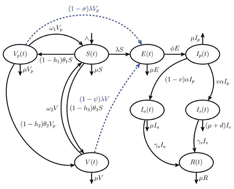
Figure 1. Schematic representation of COVID-19 model that incorporates a single-dose and a double-dose vaccination strategies that are coupled with vaccine hesitancy. The population N(t) is stratified into eight mutually exclusive classes: susceptible S(t), partially vaccinated with one dose Vp, fully vaccinated with either double-dose or single-dose vaccine V(t), exposed E(t), pre-symptomatic Ip(t), truly asymptomatic Ia(t), symptomatic Is(t), and recovered R(t). Blue dashed arrows indicate breakthrough infections.
Considering the aforementioned model description and assumptions, the system of non-linear differential equations (1) governs the transmission dynamics of COVID-19 in the presence of a single-dose and two-dose vaccines that are non-mandatory and takes into account vaccine hesitancy. A detailed description of the model parameters is captured in Table 1.
where λ remains as previously defined. The model equation (1) is subject to the initial conditions
Note that the dynamics of model equation (1) is not affected by the last equation that models the time evolution of the recovered class. Hence, the qualitative dynamics of the subgroup R will not be given much attention in the theoretical analysis.
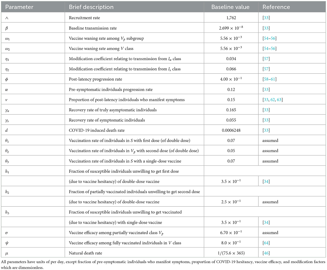
Table 1. Description of model baseline parameter values.
In this section, the model is qualitatively analyzed. First, it is shown that the model state variables remain non-negative for all time t > 0 whenever non-negative initial conditions are supplied into the system (1). Boundedness of the model trajectories will be established. The intrinsic COVID-free equilibrium and the fundamental threshold that determine the severity of COVID-19 (control reproduction number) will be determined. It will be shown that the disease-free equilibrium of the model described in section 2 is locally (globally) asymptotically stable whenever the control reproduction number is less than unity. Finally, the endemic equilibrium point together with the relevant properties (local stability) will be established.
Given the proposed model considers a human population, it is important to show the well possessedness of the model. The following theorem establishes that the model solutions remain non-negative over all the time.
Theorem 1. If the model equations (1) is supplied with positive initial conditions; S(0), Vp(0), V(0), E(0), Ip(0), Ia(0), Is(0), and R(0), then the model state variables; S(t), Vp(t), V(t), E(t), Ip(t), Ia(t), Is(t), and R(t) will always remain positive for all time, t > 0.
Proof: Suppose
First let 0 < T < +∞. Now considering continuity of solutions, we can have S(T) = 0 or Vp(T) = 0 or V(T) = 0 or E(T) = 0 or Ip(T) = 0 or Ia(T) = 0 or Is(T) = 0 or R(T) = 0. Supposing S(T) = 0 before all other state variables Vp, V, E, Ip, Ia, Is, R become zero. Then from the first equation of model system (1) we have
If Vp(T) becomes zero before all other state variables S, V, E, Ip, Ia, Is, R, then from the second equation of model system (1) we have
Following a similar procedure as described in equations (3) and (4), it is not difficult to deduce from third, fourth, fifth, sixth, seventh, and eighth equations of model system (1) the following results;
which completes the proof by showing that all the state variables of the model system (1) remain positive for all time.
Theorem 2. Define the following biologically feasible region:
Then, the region Δ is positively invariant with respect to the model system (1).
Proof: Noting that the total population is given by the sum of the state variables of the proposed model, we have
The derivative of equation (5) is given by
From equation (6), we have which can be written as Applying integration factor method and after algebraic manipulation leads to
From (7), we can deduce that Hence, it follows that as t → ∞. Thus, all the solutions of model equation (1) remain in Δ for all time which implies that the model system (1) is positively invariant. Hence, all the analysis conducted on the model system (1) are limited in the region Δ, where the model equation (1) is considered as being mathematically and epidemiologically meaningful.
In the absence of any COVID-19 infection in the community (i.e., E= Ip = Ia = Is = 0), the model system (1) has an intrinsic COVID-free equilibrium which is obtained by setting the right-hand side of equation (1) to zero. This results to
where
The basic reproduction number often denoted by is one of the important thresholds in mathematical epidemiology due to its ability in predicting the transmission dynamics of an infectious disease. It is defined as the number of secondary infectives triggered by a single primary infection during infectious period when introduced into an entirely susceptible population. For the proposed COVID-19 model equation (1), instead of computing reproduction number we compute the control reproduction number due to the reason that intervention measures for mitigating the spread of the pandemic are incorporated (vaccination strategies: single-dose and double-dose vaccines). Using the next-generation approach originally described in Van den Driessche and Watmough [65], we compute the control reproduction number as the dominant eigenvalue (spectral radius) of the next-generation matrix The matrices and respectively, represent Jacobian matrices of the terms that involve new infections and the transition rates (from one healthy status to another) computed at the COVID-free equilibrium [see Van den Driessche and Watmough [65]]. Thus, we have
and
The control reproduction number of the model system (1) can now be determined from , where ϱ is the spectral radius or the dominant eigenvalue.
Let
where
Following the theorem proved in Van den Driessche and Watmough [65], we state the following lemma.
Lemma 1. The COVID-free equilibrium of the model system (1) is LAS (locally asymptotically stable) when and unstable if
It is easy to note that the control reproduction number (10) is a sum of three terms, namely, , and Epidemiologically, represents the reproduction number of infectious individuals generated due to infection with pre-symptomatic infectious individuals in the subgroup Ip, , accounts for the reproduction number of infectious cases produced by infection with truly asymptomatic infectious individuals in the compartment Ia, and is the reproduction number associated with the number of infection cases generated as a result of infection with symptomatic infectious individuals in the subgroup Is. Mathematically, and can be expressed in terms of , that is, and Consequently,
For biologically plausible non-negative parameter values (see Table 1), both and are less than one. If both and then This indicates that the reproduction number associated with pre-symptomatic individuals is larger than both and Epidemiologically, this implies that pre-symptomatic individuals pose a greater risk as far as the spread of COVID-19 is concerned. This was not captured in several mathematical models due to the fact that it was not clear whether pre-symptomatic individuals played any significant role in the spread of COVID-19, and therefore, transmission of COVID-19 by pre-symptomatic individuals was overlooked. However, now there is a global consensus (and research still being conducted) that pre-symptomatic individuals (individuals at post-latency stage) are more infectious before symptoms start to manifest [see WHO [2] and Alleman et al. [8] and also the recent research that incorporated pre-symptomatic transmission in the force of infection [33]].
Lemma 1 implies that there is a possibility of COVID-19 pandemic being eradicated in case the initial sizes of the state variables of model equation (1) are in the basin of attraction of the COVID-free equlibrium However, there is a caveat regarding local stability of , given the proposed model system (1) assumes the COVID-19 vaccines (both single dose and double dose) being administered are not perfect. To be certain COVID-19 pandemic eradication is not dependent on the initial sizes of the state variables, we investigate whether the is globally asymptotically stable (if not, then we cannot rule out occurrence of other complex bifurcation structures, particularly backward bifurcation which occurs when ).
To analyze the global stability of model equation (1), we apply the procedure described by Castillo-Chavez et al. [66], where the two conditions that need to be fulfilled for the global asymptotic stability of the disease-free equilibrium are outlined. First, we re-write the model system (1) into the following form:
where represents the number of uninfected state variables, and represents the number of infected state variables for model system (1). Let define the COVID-free equilibrium of the proposed model (1). Then, the conditions outlined below must be fulfilled for the model system (1) to be globally asymptotically stable.
1. For Z* is g.a.s (globally asymptotically stable).
2. G2(Z, P) = AP − Ĝ2(Z, P), Ĝ2(Z, P) ≥ 0, where
represents a matrix whose off-diagonal entries are non-negative (M-matrix). Supposing conditions (i) and (ii) stated above hold in model system (1), then the following theorem follows:
Theorem 3. Assuming conditions (i) and (ii) above hold and then the fixed point is a g.a.s equilibrium point of model system (1).
Proof: It is straight forward to observe that
where Now Ĝ2(Z, P) = AP − G2(Z, P) is given as:
As t → ∞, the total population N is bounded above by which implies that the state variables S, Vp, and V satisfy the inequalities: and Consequently, after algebraic manipulation, we have
It is clear that the first terms inside the brackets in equations (14), (15), and (16) are all less than one, which implies and V0 − V < 0. The implication of this is that Ĝ2(Z, P) ≱ 0. Hence, condition (ii) for global asymptotic stability is not satisfied. Thus, the COVID-free equilibrium is not globally asymptotically stable. This signals a possibility of occurrence of bistability phenomenon where multiple equilibria coexist when the control reproduction number is less than unity. In what follows, we investigate the persistence of COVID-19 pandemic in the population through determining the endemic equilibrium point of model system (1).
In this subsection, we determine the endemic equilibrium points of model system (1) by considering that the COVID-19 is persistent in the population. Thus, we set the right-hand side of equation (1) to zero and evaluate for steady states (note the steady state R* has been omitted due to the fact that the model dynamics of equation (1) do not depend on state variable R). For the purpose of mathematical simplification, the endemic equilibrium is expressed in terms of the force of infection, which at equilibrium is denoted by Let D1 and D2 remain as previously defined in equation (9), then we define
Now, the steady states expressed in terms of force of infection at equilibrium are given as
Substituting , and into the force of infection at equilibrium yields the following fourth degree polynomial expressed as a function of λ*
where
In equation (18), λ* = 0 corresponds to COVID-free equilibrium Hence, the possible number of endemic equilibria for model system (1) is obtained by evaluating for λ* in the following third-degree polynomial
and substituting the corresponding roots in (17). It is straightforward to note that if the vaccines administered are imperfect (i.e., σ, ψ < 1), then C3 is always positive while C0 can be positive/negative depending on whether the control reproduction number is less/greater than unity. Note that for C0 reduces to zero. The number of endemic equilibria for the cubic polynomial (20) has been comprehensively studied using the technique by Descartes, usually referred as Descartes rule of signs [67]. Supplementary Table S1 (in the Supplementary Material S1) gives the possible number of COVID-19 persistent equilibria and the corresponding type of bifurcation structure.
For a perfect vaccine (i.e., σ = ψ = 1, ω1 = ω2 = 0), C3 and C2 become zero leading to the following linear equation:
where
Solving linear equation (21) yields
Hence, equation (21) has a unique positive root λ** whenever and a negative root whenever The epidemiological implication of non-existence of a positive endemic equilibrium point when is that it is sufficient to eradicate COVID-19 pandemic by implementing control strategies that decrease control reproduction number below one. That is, for vaccines (both single-dose and double-dose vaccines) with 100% effectiveness against COVID-19, the model system (1) has a unique endemic equilibrium point which we shall denote by that is globally asymptotically stable whenever Thus, the following theorem follows.
Theorem 4. Provided the vaccine is perfect (i.e., σ = ψ = 1, ω1 = ω2 = 0) and , the unique endemic equilibrium point is globally asymptotically stable.
Proof: Using the well-known scalar function for investigating global stability [68] [see also the recent study [69] where an auxiliary function has been used], we define the following Lyapunov candidate function:
The orbital derivative of (22) is given by
At equilibrium, the following equalities hold:
Substituting (26) in (25) and simplifying yields
The fifth, sixth, seventh, and eighth terms in equation (27) together with further explanation in Supplementary Material [S2] can be re-written as follows:
Substituting inequalities (29)-(33) in (27) leads to
Considering the fact that the geometric mean is smaller than the arithmetic mean, it follows that with equality holding (i.e., ) if and only if and Hence, is a suitable Lyapunov function in the region Δ, and the unique endemic equilibrium is globally asymptotically stable when This implies that if the vaccines being administered are perfect, all trajectories of model system (1) whose initial conditions are in the region Δ eventually converge to the unique endemic equilibrium point as t → ∞ provided Epidemiologically, it means that model system (1) cannot exhibit the phenomenon of backward bifurcation if the vaccine efficacy is 100% and everlasting.
Theorem 4 implies that in case the vaccines administered are perfect and livelong, then the model system (1) cannot have the phenomenon of backward bifurcation. In this subsection, we relax the possibility of a perfect and everlasting vaccine but instead investigate model dynamics in presence of an imperfect vaccine.
To investigate whether the model system (1) exhibits bistability phenomenon, we apply the center manifold theory as descrbed by Castillo-Chavez et al. [70]. Given at the point is where there is change in bifurcation structure, we choose β = β* as our bifurcation parameter where β* is obtained by setting and evaluating for β. That is
For the purpose of simplification, we re-write model system (1) using new variables denoted by S = x1, Vp = x2, V = x3, E = x4, Ip = x5, Ia = x6, Is = x7) and the total population size Let (T denotes transpose), which implies where F = (f1, f2, f3, f4, f5, f6, f7). With the new variables, the Now, we define the model system (1) as follows:
The Jacobian matrix of model (36) evaluated at is given by:
where and
Now, the right eigenvector corresponding to the zero eigenvalue of the Jacobian matrix is obtained as where
Similarly, the left eigenvector corresponding to the zero eigenvalue of is given by where
As described in Theorem 4.1 of Castillo-Chavez [70], the type of bifurcation structure exhibited by the model is determined by the bifurcation coefficients, a and b which are defined as
Computations involving parameter a: Now, we proceed and determine the non-vanishing partial derivatives evaluated at the COVID-free equilibrium of model equation (36). These partial derivatives include:
Hence,
Computations involving bifurcation parameter b: The bifurcation parameter b is associated with the following non-vanishing partial derivatives evaluated at
Hence,
Note that the eigenvectors and ṽ5 are always positive and Q0 > 0; hence, b is non-negative. For backward bifurcation to occur, we need both a and b to be positive. Notice that the bifurcation parameter a is positive if Γ1 > Γ2. Thus, backward bifurcation can occur if the inequality
holds. In case vaccines are perfect and permanent, (i.e., σ = ψ = 1, ω1 = ω2 = 0) Γ2, P2 are equal to zero while Γ1 reduces to
where
The observations that a < 0 when vaccines administered are assumed to be perfect and everlasting (i.e., ψ = σ = 1, ω1 = ω2 = 0) agree with the global asymptotic stability results proved in Theorem 4. However, if the vaccines administered among susceptible and partially vaccinated cohorts are imperfect and non-permanent hence, allowing for breakthrough infections to occur, the well-known backward bifurcation phenomenon [71–73] may arise. The epidemiological implication of the occurrence of backward bifurcation is that it will be more difficult for implemented intervention measures to eliminate the COVID-19 pandemic. This is due to the fact that reducing below unity will be necessary but not sufficient. Thus, following the above bifurcation analysis, we state the following result:
Theorem 5. Provided the inequality given by (37) holds, the COVID-19 model system (1) exhibits backward bifurcation phenomenon when crosses unity.
To gain insight on the most effective combination of mitigation strategies that can be adopted to significantly minimize the spread of COVID-19 pandemic as well as the cost, we introduce three time-dependent control measures that are broadly categorized as either non-pharmaceutical (NPIs) and pharmaceutical control measures. Thus, the proposed model (1) is transformed to an optimal control COVID-19 infection model. The non-pharmaceutical time-dependent COVID-19 control is denoted by u1(t), which represents preventive control measures that involve social/physical distancing, wearing face mask, hand washing, and adherent to education on proper hygiene among susceptible, partially vaccinated (with a double-dose vaccine) and fully vaccinated individuals (with either double-dose or single-dose vaccine). The pharmaceutical time-dependent intervention measures include u2(t) which represents a time-dependent screening-management control measure for infectious individuals in the subgroups Ia and Is, and θ3(t) which represents time-dependent vaccination control for susceptible individuals with a single-dose vaccine. Incorporating these time-dependent control measures, the model system (1) transforms to the following non-linear (also non-autonomous) system of ordinary differential equations:
In model system (38), the parameter c accounts for control rate constant while the terms 1 − u1(t), θ3(t), and u2(t) are the controls that aim to curb the spread of the COVID-19 pandemic over a long time scale. Note that u1, θ3, u2 ∈ [0, 1]. Given the objective of time-dependent control measures is to attempt to mitigate the proliferation of COVID-19 pandemic and eventually eradicating it by; minimizing the sub-populations of infectious individuals and also minimizing the cost of mitigation strategies, we define the objective functional as
where Tf denotes the terminal time such that t ∈ [0, Tf] while and (j = 1, 2, 3) represent weight constants. The term is the cost associated with adopting non-pharmaceutical intervention measures which include social/physical distancing, wearing face masks, hand washing, and adhering to proper hygiene education among individuals in the subgroups S, Vp, and V, and is the cost associated with vaccination of susceptible individuals with a single-dose vaccine. Furthermore, the term is the cost associated with COVID-19 screening-management for both individuals in Ia and Is compartments. The choice of a quadratic cost function is motivated by the relevant literature in the sequel on optimal control problems [for instance, see Okyere et al. [74], Ghosh et al. [75], Bonyah et al. [76], Purwati et al. [77], Lenhart and Workman [78] and Olaniyi et al. [79]]. Thus, we now proceed to find a which fulfills
where is a Lebesgue measurable control set which has a lower bound as zero and an upper bound 1 for t ∈ [0, Tf].
Following Pontryagin's maximum principle originally described in Pontryagin [80], we establish the necessary conditions that an optimal control COVID-19 model system (38) needs to fulfill. The technique outlined by Pontryagin et al. [80] enables conversion of the model system (38) in synergy with the objective functional (39) into a problem of minimizing pointwise a Hamiltonian with respect to the time-dependent control measures; u1(t), θ3(t), u2(t). Consequently, we define the Hamiltonian of model system (38) as
where y = (S, Vp, V, E, Ip, Ia, Is, R) represents COVID-19 model state variables, is a Lagrangian which represents the integrand of the objective functional, and λj represents the corresponding adjoint variables for the model states S, Vp, V, E, Ip, Ia, Is, R. Moreover, qj is the right-hand term of the model system (38). Thus, the Hamiltonian is stated explicitly as
We now establish the following results:
Theorem 6. Assuming a solution of the optimal control problem for the objective functional over the control set V is obtained, then the adjoint variables λ1, λ2, ⋯ , λ8 fulfill the adjoint equations
with λj(Tf) = 0 as transversality condition and y = (S, Vp, V, E, Ip, Ia, Is, R). Moreover, optimal controls are given as
where
Proof: Let By Pontryagin's maximum principle, the state variables of the model (38) and adjoint variables satisfy the following relations which are obtained from the Hamiltonian
That is, the adjoint equations can now be expressed as
with the transversality conditions:
Further in the interior of the set where the controls are bounded in 0 ≤ u1, θ3, u2 ≤ 1, we have the following optimality conditions being satisfied:
such that
Given the time-dependent controls are bounded below by zero and above by one, we summarize the characterization as
where j = 1, 2, 3; and
To validate theoretical findings of model system (1), we perform numerical simulations using MATLAB so as to gain more insight on equilibrium dynamics as well as on time profiles. Analytical analysis of the persistent COVID-19 equilibrium indicates that the model exhibits the phenomenon of backward bifurcation when certain conditions are satisfied as shown in Theorem 5, that is, if the double-dose and single-dose vaccines being administered are not 100% effective against suppressing COVID-19 persistent, then there exist a set of parameters that if they fulfill the condition that Γ1 > Γ2, and then bistability phenomenon arises. Hence, plotting the solution of cubic equation (20) (i.e., force of infection at equilibrium) as a function of the effective contact rate β results to Figure 2A which clearly depicts the phenomenon of backward bifurcation where COVID-19 persists even when the control reproduction number is below unity. The epidemiological implication of the occurrence of backward bifurcation signals that it will not be sufficient to decrease below unity. Figure 2B which is obtained by varying vaccine efficacy among fully vaccinated individuals while all other parameters remain fixed as in Table 1 shows that vaccine with high efficacy leads to reduction of control reproduction numbers , , , and Figure 2B also corroborates with theoretical findings in equation (11) where it is shown that infectious pre-symptomatic individuals contribute significantly in the increase of control reproduction number in comparison with truly asymptomatic and symptomatic infectious individuals. In fact, curve is higher than and curves for any given plausible set of parameter values.
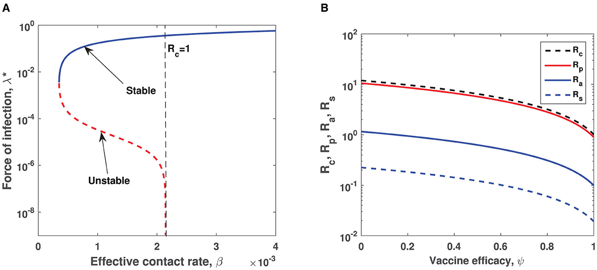
Figure 2. (A) Illustration of the backward bifurcation phenomenon when vaccine is assumed to be imperfect. Parameters used are same as those in Table 1 except h1 = 0.1, h2 = 0.85, h3 = 0.01, θ1 = 0.015, θ2 = 0.68, θ3 = 0.075, σ = 0.5, v = 0.1, γa = 0.000165, γs = 0.00055, d = 0.001, ∧ = 0.0001which correspond to Γ1 = 0.0056 > Γ2 = 0.0049. Semi-logarithmic scale is used for a better view of bifurcation curves. The red dotted curve represents the unstable curve, while blue solid curve represents the stable curve. (B) Impact of vaccine efficacy ψ on control reproduction numbers. Semi-logarithmic scale is used for a clear view.
The COVID-19 model proposed adopted two vaccination strategies, that is, vaccinating susceptible individuals with either single-dose or double-dose vaccines. The parameters that relate to vaccination rates are θ1, θ2, and θ3 where θ1 and θ2 represent first dose and second dose vaccination rates for a double-dose vaccine while θ3 is the vaccination rate for a single-dose vaccines. While both strategies remain important in suppression of COVID-19 over a long time scale, it is worth investigating which strategy has more positive impact in mitigating COVID-19. Hence, fixing all other parameters constant as indicated in Table 1 while switching on and off vaccination rates, we obtain Figures 3A–D. Figure 3 reveals that single-dose vaccination strategy leads to a significant decline in COVID-19 prevalence in comparison with a double-dose vaccination strategy and baseline scenario (no vaccination). It is important to stress that these simulation results were generated when vaccine hesitancy is assumed to be equal among susceptible and partially vaccinated individuals (i.e., h1 = h2 = h3 = 0.35). Hence, in a setting where vaccine reluctance (vaccine hesitancy) is more likely to occur, single-dose vaccination strategy would be more recommendable than a double dose-vaccine. This is due to the fact individuals who receive first dose of the double-dose vaccine may choose not to receive second dose as a result of vaccine hesitancy. The advantage of administering a single-dose vaccine is that vaccine hesitancy among partially vaccinated individuals is circumvented. Furthermore, it is important to note that both single-dose and double-dose vaccination strategies lead to a delay in COVID-19 peak when compared with the baseline scenario (no vaccine) indicated by a solid black curve in each figure. Interestingly, when comparing delay in COVID-19 peak between single-dose and double-dose vaccination strategies, there is no significant difference. In contrast, if both vaccination strategies are concurrently implemented, there is considerable difference in both COVID-19 prevalence and delaying in COVID-19 peak (when compared with baseline scenario and either single-dose or double-dose epidemic curve). That is, for the case of combined vaccination strategies, the epidemic curve is more flattened (see Figure 3). Thus, administering both single-dose and double-dose vaccines simultaneously has a positive impact in diminishing COVID-19 proliferation. Furthermore, a more flattened epidemic curve implies minimal burdening of healthcare infrastructure, given there will be no sudden surge of severely ill COVID-19 patients who need hospitalization.
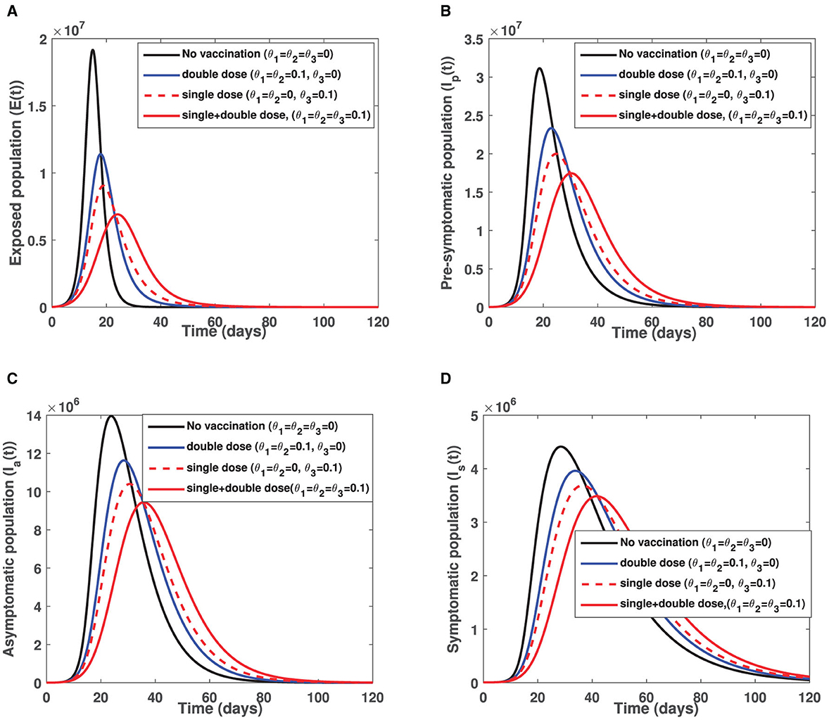
Figure 3. Illustrate impact of single dose and double dose vaccination strategies on (A) the exposed individuals (B) pre-symptomatic infectious individuals (C) truly asymptomatic infectious individuals and (D) symptomatic infectious individuals. Parameters used remain as shown in Table 1 except, θ1, θ2, and θ3 which are shown in the figure while initial conditions used are S(0) = 60000000, Vp(0) = 0, V(0) = 0, E(0) = 10954, Ip(0) = 10954, Ia(0) = 7322, Is(0) = 7545, R(0) = 203968.
It is worth noting that despite COVID-19 vaccines being administered in almost every country in the world, the unwillingness of the general populace to accept COVID-19 jabs impend intervention measures put in place to end the COVID-19 pandemic. To elucidate on the impact of vaccine hesitancy on the COVID-19 transmission dynamics, we fix vaccination rates among susceptible and partially vaccinated individuals to a constant value (i.e., θ1 = θ2 = θ3 = 0.1) and vary the fraction of individuals unwilling to receive COVID-19 jabs. That is, h1, h2, h3 ∈ [0, 0.25, 0.50, 0.75, 0.90] while all other parameters remain as defined in Table 1. The first row figures of Figure 4 present the direct consequence of unwillingness to receive double-dose vaccine (by susceptible and partially vaccinated individuals) on the sizes of the infectious populations Ip, Ia, and Is. The second row figures of Figure 4 show effect of unwillingness to receive single-dose vaccine (by the susceptible populations) on the sizes of infectious subgroups Ip, Ia, and Is. The last row of Figure 4 shows the combined impact of vaccine hesitancy against single-dose and double-dose vaccines on the infectious cohorts Ip, Ia, and Is. Figures 4A–C depict that an increase in vaccine hesitancy against single-dose vaccine has an adverse effect on COVID-19 prevalence. This is due to an increase in infectious population sizes (i.e., pre-symptomatic, truly asymptomatic and symptomatic) as vaccine hesitancy increases. An increase in infectious population sizes translates to an increase in likelihood of coming into contact with an infectious person which ultimately leads to more positive cases being confirmed in any given setting. Vaccine hesitancy against double-dose vaccine triggers an early appearance of COVID-19 peak among pre-symptomatic population than on both truly asymptomatic and symptomatic individuals. This observation is epidemiologically crucial, given in several epidemiological models the contribution of pre-symptomatic individuals in transmission of COVID-19 was ignored.
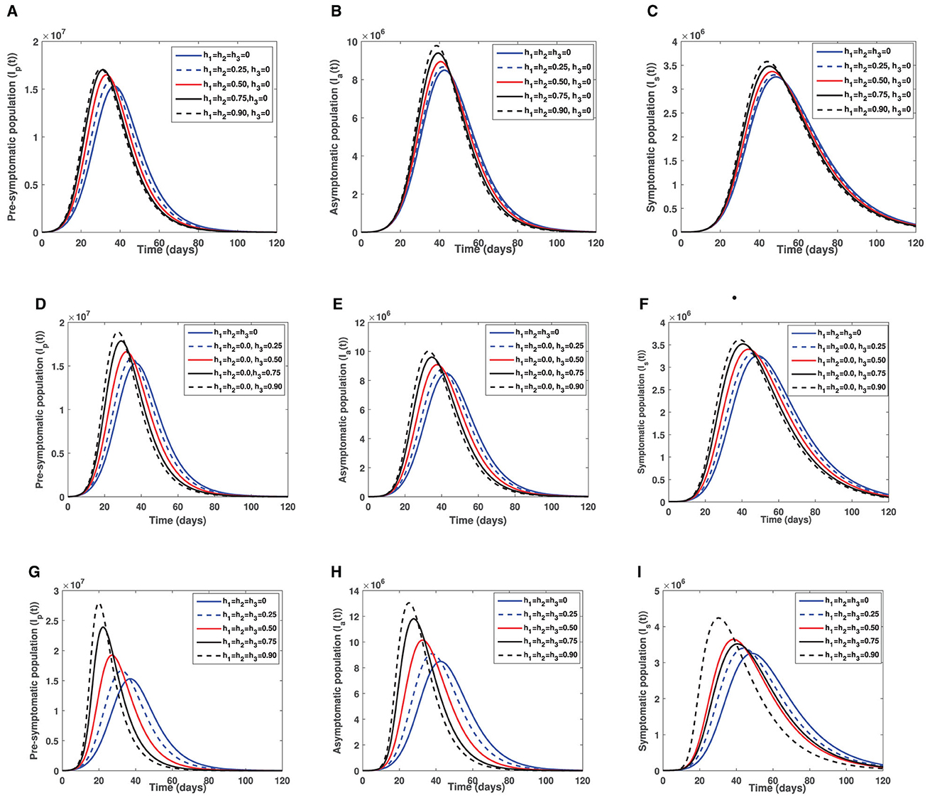
Figure 4. Illustrate the effect of vaccine hesitancy against double-dose vaccine, single-dose and both vaccines. (A) Show the effect of vaccine hesitancy against double-dose on pre-symptomatic infectious individuals. (B) Show the effect of vaccine hesitancy against double-dose on infectious truly asymptomatic individuals. (C) Illustrate the effect of vaccine hesitancy against double-dose on infectious symptomatic individuals. (D) Depict the effect of vaccine hesitancy against single-dose on pre-symptomatic infectious individuals. (E) Show effect of vaccine hesitancy against single-dose on infectious truly asymptomatic individuals. (F) Represents effect of vaccine hesitancy against single-dose on infectious symptomatic individuals. (G) Show the impact of vaccine hesitancy against both single and double dose on pre-symptomatic infectious individuals. (H) Show the impact of vaccine hesitancy against both single-dose and double-dose vaccines on infectious truly asymptomatic individuals. (I) Show the impact of vaccine hesitancy against both single dose and double dose vaccines on infectious symptomatic individuals. The blue solid epidemic curve represents the baseline scenario where there is no vaccine hesitancy.
Figures 4D–F present a scenario where there is vaccine hesitancy against single-dose vaccine (by susceptible individuals). It is observed that unwillingness to receive single-dose vaccine by susceptible individuals is more detrimental than vaccine hesitancy against double-dose vaccine. This is due to the pronounced early appearance of COVID-19 peaks among all the three infectious populations (Ip, Ia, Is) and a wider increase in COVID-19 prevalence when compared to a case of vaccine hesitancy against double dose (see Figures 4A–C). Again, an early peak of COVID-19 epidemic curve is more notable among pre-symptomatic population than on both truly symptomatic and symptomatic populations. The combined impact of vaccine hesitancy against both single-dose and double-dose vaccines (by both susceptible and partially vaccinated cohorts) is presented in Figures 4G–I. It is clearly visible from Figures 4G–I that vaccine hesitancy against both single-dose and double-dose vaccines is disastrous as there is a rapid increase in COVID-19 prevalence by a wider margin when compared with the baseline curve (see the blue solid curve in each figure of Figure 4). Furthermore, a rise in vaccine hesitancy against the two vaccines being administered (single dose and double dose) triggers an early peak of COVID-19 epidemic curve which is again more pronounced when compared with vaccine hesitancy against each vaccination strategy (either single or double dose).
To visualize the impacts of each of the three time-dependent controls and the effects of combining any two of the controls on the dynamics of COVID-19 transmission [81], we simulate the optimality system comprising the state system (38) and the adjoint system (45). Keeping in mind that the optimality system is a two-point boundary problem with both initial and transversality conditions (2) and (47), respectively, we therefore make use of fourth-order forward-backward Runge-Kutta method. We first solve the state system (38) forward in time with the initial condition (2) after initial guessed values for the controls. Then, we solve the adjoint system (45) backward in time with the transversality conditions (47) and update the controls using a convex combination of both the initial guessed values and current values of the control characterizations (48). We continue this iteration until the absolute error between the current and previous solutions of the optimality system is negligibly small [78, 82, 83]. The simulation is performed using MATLAB over the time interval [0, 120] days with the following initial conditions: S(0) = 60000000, Vp(0) = 0, V(0) = 0, E(0) = 10954, Ip(0) = 10954, Ia(0) = 7322, Is(0) = 7545, R(0) = 203968. We use the same parameter values given in Table 1 together with the weight and rate constants , (m = 1, 2, 3), , (n = 1, 2, 3), and c = 1.
As shown in Figure 5, implementation of the non-pharmaceutical time-dependent control u1(t) reduces the populations of pre-symptomatic, asymptomatic, and symptomatic individuals. The control profile shows that the non-pharmaceutical measure should be adhered to at maximum value for almost the implementation period to flatten the infectious curves. In Figure 6, we see that administration of the optimal vaccination control θ3(t) for susceptible individuals with a single-dose vaccine helps in reducing the sizes of individuals in the subgroups Ip, Ia, and Is when compared with the case without vaccination control.
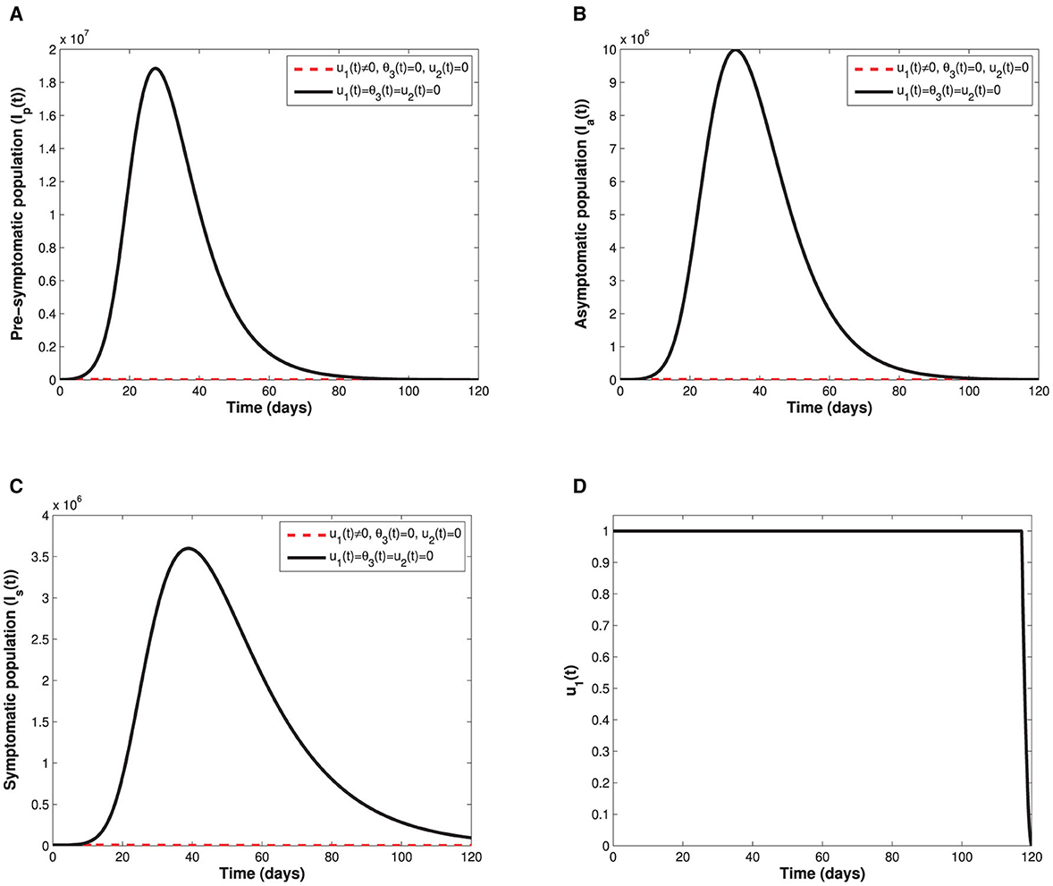
Figure 5. Depict the impact of the non-pharmaceutical control u1(t) on; (A) the infectious pre-symptomatic population. (B) The infectious truly asymptomatic population. (C) The infectious symptomatic population. (D) Represents the control profile of time-dependent control u1(t).
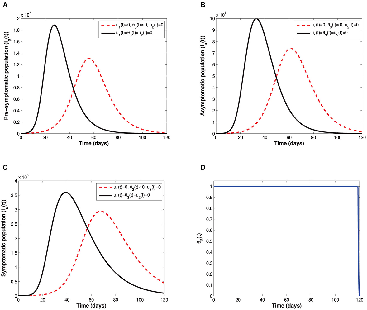
Figure 6. Depicts the impact of the time-dependent optimal vaccination control θ3(t) on: (A) the infectious pre-symptomatic population. (B) The infectious truly asymptomatic population. (C) The infectious symptomatic population. (D) Represents the control of time-dependent optimal vaccination control θ3(t).
Since the time-dependent management control u2(t) is only targeted at the populations of asymptomatic and symptomatic individuals, Figure 7 therefore displays the behaviors of the subgroups Ia and Is in the presence and absence of u2(t). It can be seen that the sizes of both asymptomatic and symptomatic individuals with control are lower when compared with the sizes without control. The control profile also indicates that management of infectious cases in the population should be sustained at maximum throughout the implementation period. Moreover, control profiles showing the combination of u1(t) and θ3(t), and the combination of u1(t) and u2(t) are displayed in Figure 8. In both profiles, we see that the non-pharmaceutical measure u1(t) is maintained at maximum for almost 100% of the implementation period, while each of vaccination and management controls is maintained at maximum for 30% and 72% of the total implementation period, respectively. This implies that whenever the non-pharmaceutical measure is fully adhered to, less effort will be needed by either vaccination or management control to achieve optimal reduction of COVID-19 spread. Lastly, the influence of combination of both θ3(t) and u2(t) on the populations of individuals in the subgroups Ip(t), Ia(t), and Is(t) is shown in Figure 9. We see that both vaccination and management controls are to be sustained at maximum throughout the required implementation period to reduce the sizes of infectious individuals in the population.
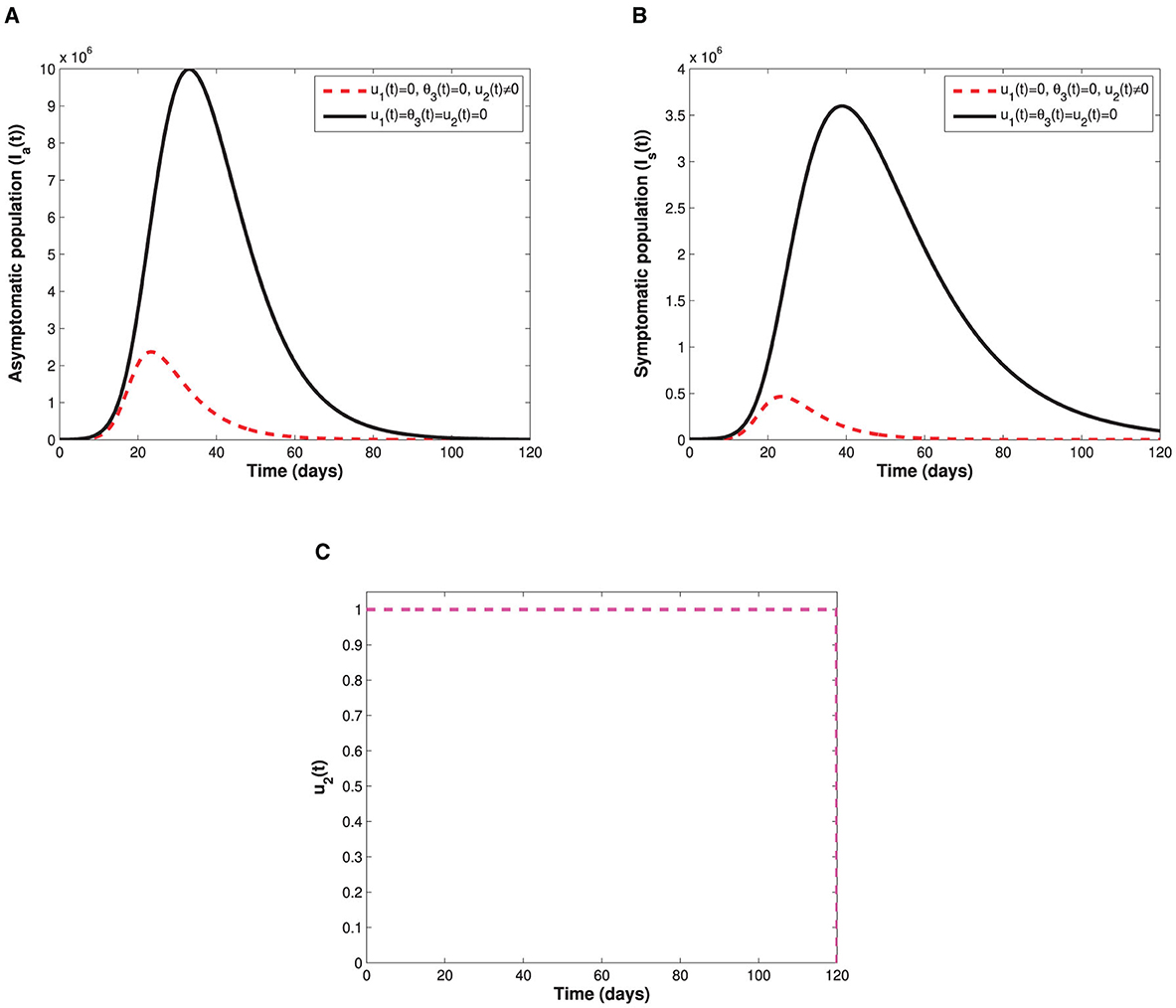
Figure 7. Illustrate the impact of the time-dependent screening-management control measure u2(t) on: (A) the infectious truly asymptomatic population. (B) The infectious symptomatic population. (C) Represents the control profile of time-dependent screening-management control measure u2(t).
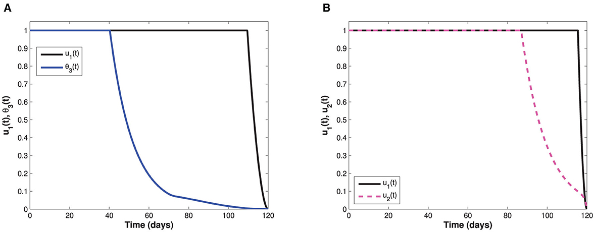
Figure 8. Represents control profiles involving combinations of non-pharmaceutical measure with each of the optimal vaccination and management controls. (A) Represents control profiles for both optimal non-pharmaceutical control measure and optimal vaccination measure. (B) Represents control profiles for both optimal non-pharmaceutical control measure and screening-management control.
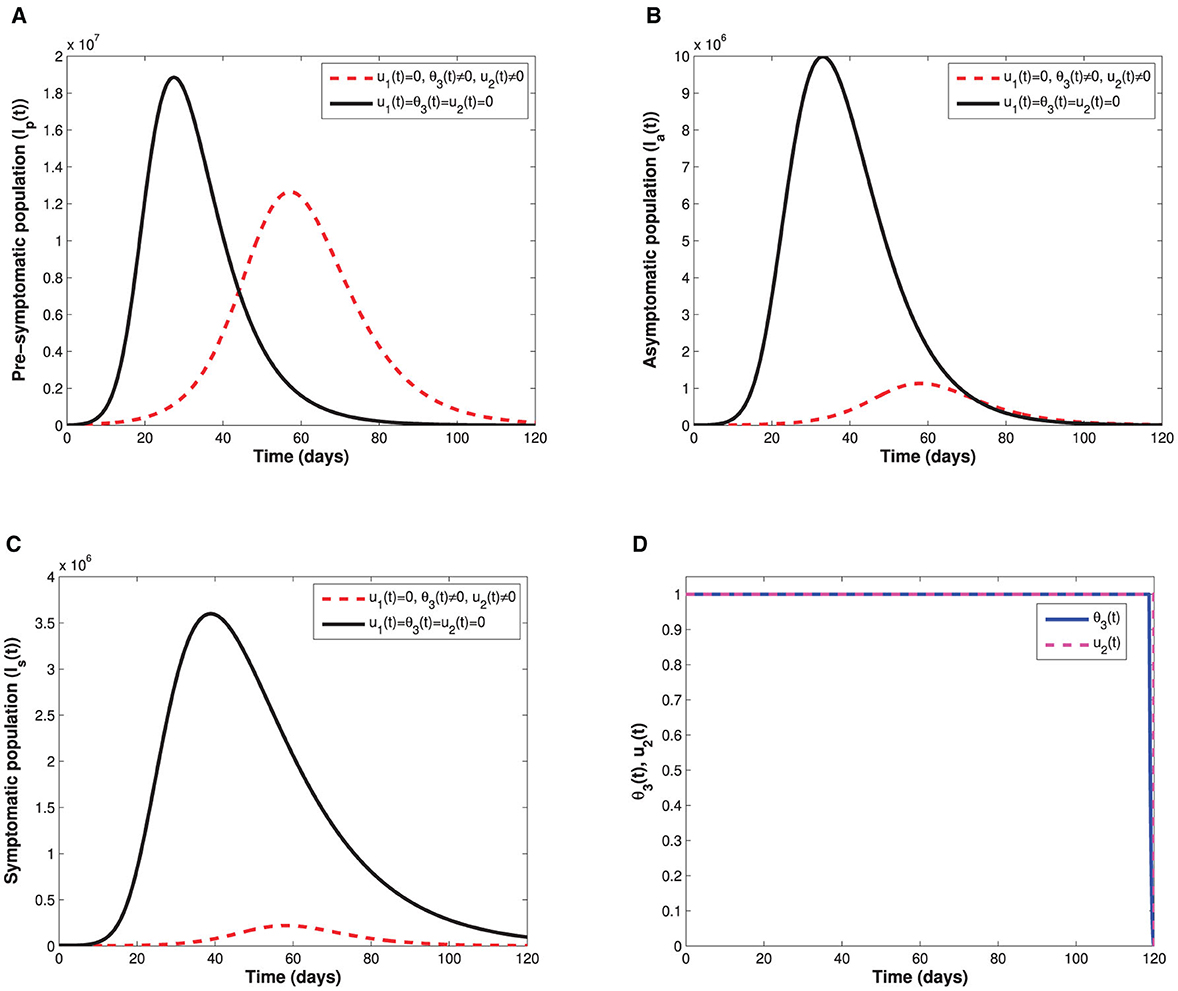
Figure 9. Demonstrate impact of combining the time-dependent optimal vaccination θ3(t) and management u2(t) controls on: (A) the infectious pre-symptomatic population (B) The infectious truly asymptomatic population (C) The infectious symptomatic population. (D) Represents the control profiles for both optimal vaccination and optimal screening-management of infectious individuals.
Out of the single and several combinations of controls considered in this study, it is important to identify the main control strategy which minimizes COVID-19 transmission optimally at the lowest cost of implementation when available resources are limited. To do this, we make use of the two known methods, namely, average cost-effectiveness ratio (ACER) and incremental cost-effectiveness ratio (ICER) [84–86]. ACER is measured by dividing the cost of implementing a control strategy by the total benefits of such strategy in terms of cases averted. It is given by
Unlike ACER, we use ICER to compare effectiveness of any two competing control strategies, and it is measured by finding the ratio of the difference between the costs of the two strategies to the difference between their health benefits. The ICER is calculated using
As a result of the numerical simulations of the optimal control problem, we now present the values of the cases averted by each of the control strategies in an increasing order with their corresponding costs of implementation. We have used 49 and 50 to calculate ACER and ICER, respectively, as shown in Table 2.
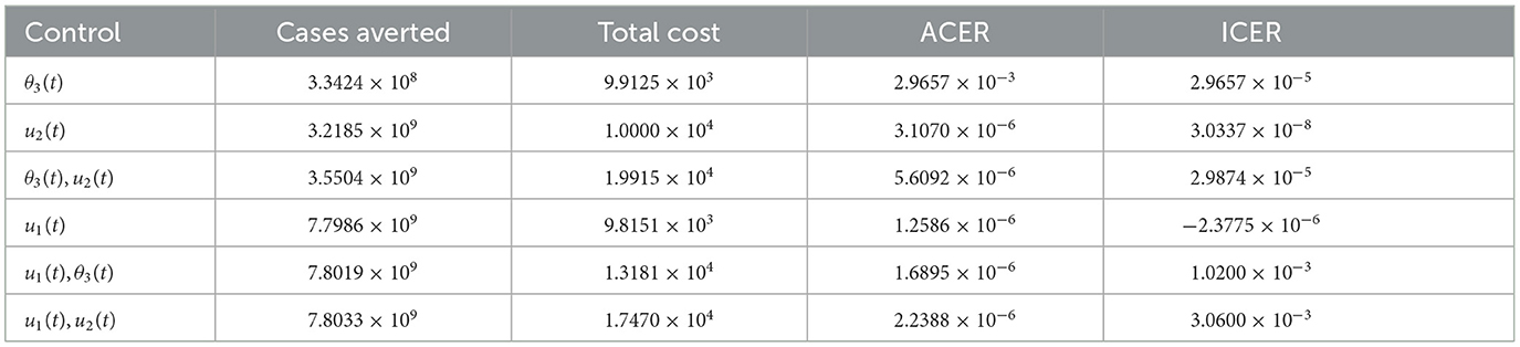
Table 2. Increasing order of COVID-19 cases averted by control strategies.
It can be observed that u1(t) has the least ACER value in comparison with the other control strategies. This suggests that the non-pharmaceutical control is the most cost-effective strategy that can be implemented when resources are limited. To further confirm this result, we first carry out ICER analysis between θ3(t) and u2(t), and see that ICER(θ3(t)) is greater than ICER(u2(t)). This implies that implementing vaccination control is costlier and less-effective when compared with the optimal screening-management control. Hence, the control strategy θ3(t) is excluded from the list of control strategies and we concentrate on the remaining as indicated in the Table 3.
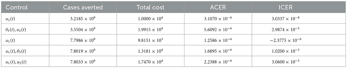
Table 3. ICER analysis without optimal vaccination control θ3(t).
Comparison between the single control u2(t) and the combination of θ3(t) and u2(t) in the Table 3 shows that ICER(θ3(t), u2(t)) is greater than ICER(u2(t)), implying that implementing the combination of both vaccination and management controls is more expensive than the single implementation of optimal management control. Thus, we remove the combination θ3(t) and u2(t) from the list of the available control strategies and continue to analyze ICER for the remaining control strategies as presented in Table 4. We see that the non-pharmaceutical control u1(t) strongly dominates the management control u2(t) since ICER(u1(t)) is less than ICER(u2(t)). Therefore, we discard the control u2(t) and re-compute ICER for the remaining strategies.

Table 4. ICER analysis without the single θ3(t) and the double (θ3(t), u2(t)).
Following similar procedure, we remove the combination of u1(t) and θ3(t) since it is strongly dominated by the single control strategy u1(t) as seen in the Table 5. Hence, we are left with two control strategies as indicated in Table 6. Consequently, the combination of u1(t) and u2(t) is removed from the analysis since ICER(u1(t), u2(t)) is greater than ICER(u1(t)). Hence, single implementation of the non-pharmaceutical control strategy is the most cost-effective of all the strategies. This result is in total agreement with the ACER result obtained earlier.
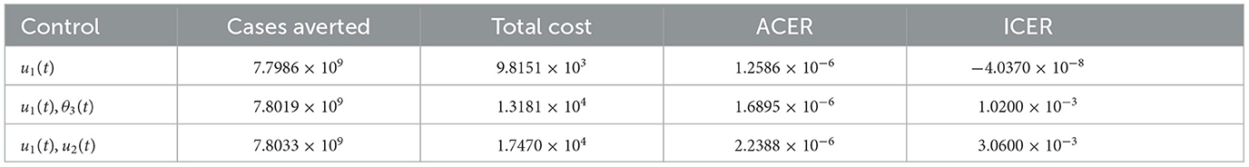
Table 5. ICER analysis without single θ3(t), double (θ3(t), u2(t)), and single u2(t).
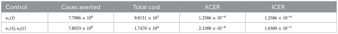
Table 6. ICER between single u1(t) and double (u1(t), u2(t)).
This study considered a COVID-19 epidemiological framework that modeled transition from one healthy status to another using a deterministic non-linear ordinary differential equations. Given vaccines are widely accepted by policymakers as an important intervention measure for curbing COVID-19 proliferation, we incorporated into the proposed model non-mandatory vaccines. Contrary to previous work [33, 35, 41–44, 46] on COVID-19, we considered a setting where susceptible individuals have a choice of either being vaccinated with a single- or double-dose vaccine. Furthermore, a fraction of individuals who initially choose double-dose vaccine refuse the second dose and therefore remain partially vaccinated (these individuals can be infected with COVID-19 upon exposure with infectious individuals). This differs with [33, 46] studies that assumed vaccinated individuals acquired sufficient vaccine-induced immunity, and therefore, they could not be infected.
The assumption that vaccinated individuals could not be infected (see [33, 46]) hindered the important epidemiological phenomenon of backward bifurcation which has been observed in this study. For instance, findings from equilibrium analysis of the model suggest that if both single-dose and double-dose vaccines administered to the general populace are perfect and permanent then intervention measures that aim to decrease control reproduction number below one will be sufficient in curbing COVID-19 (see Theorem 5). However, if vaccines administered are imperfect and non-permanent, there exists a parameter space where the phenomenon of backward bifurcation may arise leading to persistence of COVID-19 even when the control reproduction number is below one. This observation hints that policymakers (in particular governments across the world) and medical practitioners should advocate production of vaccines that render optimal efficacy (as well as vaccines that provide a livelong vaccine-induced immunity) so that breakthrough infections are prevented at all cost. The studies done by Buonomo et al. [33], Oduro et al. [35], Buckner et al. [41], Choi and Shim [42], Mukandavire et al. [43], Deng et al. [44], and Peter et al. [46] did not exhibit any bistability phenomenon. Both analytical and numerical results on the three control reproduction numbers indicate that the control reproduction number associated with the number of infectious individuals generated as a result of contact with pre-symptomatic individuals is always larger than the other two control reproduction numbers associated with symptomatic and truly asymptomatic infectious individuals, respectively. This finding is important as far as COVID-19 transmission dynamics is being demystified both at epidemiological and biological level. The revelation regarding extent of contribution of pre-symptomatic individuals can inform policymakers and medical practitioners on the importance of implementing early screening and quarantine of individuals exposed to COVID-19 to avert spiraling of COVID-19 cases. The studies conducted in Tiwari et al. [39], Rai et al. [40], Kumar et al. [48], Majumder et al. [87], srivastav et al. [88], Oduro et al. [35], Buckner et al. [41], Choi and Shim [42], Mukandavire et al. [43], Deng et al. [44], and Peter et al. [46] never captured the epidemiological implication of pre-symptomatic individuals due to the fact that they did not incorporate pre-symptomatic cohort. Also during the time of their studies, there was no universal consensus on whether pre-symptomatic individuals contributed in the spread of COVID-19 as it is now known [8].
The time profile findings reveal a profound difference in reduction of COVID-19 prevalence when either single-dose vaccine or double-dose vaccine is administered among susceptible population. Administering single-dose vaccines leads to a significant decline of COVID-19 prevalence than double-dose vaccines, especially in a setting where vaccine hesitancy is present. This epidemiologically implies that in a setting where vaccine hesitancy is rampant, a single-dose vaccine should be recommended. This is due to the fact that single-dose vaccine circumvents the second dose vaccine hesitancy likely to be witnessed among partially vaccinated individuals who may refuse second COVID-19 jab due to reasons such as mild (severe) side effects experienced with the first dose. This is despite the existing evidence from medical practitioners that the vaccine benefits considerably outweigh the risks of side effects associated with COVID-19 vaccines being administered globally. Nevertheless, in a scenario where both vaccines are simultaneously administered, there is a significant decline in COVID-19 prevalence, regardless of the level of vaccine hesitancy. It is important to stress that the findings regarding epidemiological impact of combined effect of single-dose and double-dose vaccines have not been documented in any literature (known so far) possibly due to the fact that no existing study has analyzed a model that incorporated both vaccines (single-dose and double-dose vaccines) and vaccine hesitancy simultaneously. Even the recent studies [33, 35, 41–44, 46] on COVID-19 considered only a single-dose or a double-dose vaccines separately.
Investigation on the impact of unwillingness to receive either single-dose or double-dose vaccine reveals that vaccine hesitancy triggers an early peak of COVID-19 outbreak. Sudden surge of COVID-19 prevalence implies the available medical facilities will be overburdened by severely ill COVID-19 patients who are in need of urgent medical attention. In addition, if vaccine hesitancy against both vaccines (that is single dose and double dose) is rampant in the general populace, then COVID-19 epidemic curve peaks faster than vaccine hesitancy against either a single-dose or double-dose vaccine. This implies that countermeasures put in place to control COVID-19 proliferation need to go beyond providing free COVID-19 jabs but also demystify the benefits associated with COVID-19 vaccines so as to raise the level of vaccine acceptance in the general population.
The extension of the COVID-19 model to an optimal control problem by incorporating three time-dependent controls also shed some epidemiological insights on how optimal non-pharmaceutical and pharmaceutical intervention measures may influence COVID-19 transmission dynamics. The three time-dependent controls which are broadly categorized as either non-pharmaceutical (NPIS) and pharmaceutical included preventive control measures (such as social/physical distancing, wearing face mask, hand washing, and adherent to education on proper hygiene) among susceptible and vaccinated cohorts, vaccination of susceptible individuals with a single dose-vaccine, and screening-management of infectious symptomatic individuals and truly asymptomatic individuals. Previous studies [33, 35, 41–44, 46] on COVID-19 did not consider these three time-dependent control measures as we have considered in this study; hence, findings obtained in the study are unique and different from their findings. Optimal simulation results show that if susceptible and both vaccinated cohorts (either partially vaccinated or fully vaccinated) adhere to COVID-19 non-pharmaceutical intervention measures, then COVID-19 pandemic can be easily eradicated. Thus, in the midst of a COVID-19 pandemic advising the public to adhere to non-pharmaceutical preventive measures even after vaccination can have positive impact through reduction of COVID-19 prevalence to almost zero. Furthermore, cost-effectiveness analysis has shown that non-pharmaceutical intervention control is the most effective and cheapest when compared with pharmaceutical controls (management-screening controls of symptomatic and truly asymptomatic and vaccination control). Optimal management of infectious symptomatic and truly asymptomatic individuals significantly reduces COVID-19 prevalence but does not lead to a delayed COVID-19 peak. On the one hand, optimal vaccination of susceptible individuals has 2-fold benefits, that is, reduction of COVID-19 prevalence as well as delaying the peak of COVID-19 outbreak. This allows policymakers and medical practitioners to have sufficient time to plan and manage the existing COVID-19 cases.
It is imperative to stress that there are few limitations to this study. First, data on COVID-19 vaccine hesitancy are limited, and the research that analyzed individual level of vaccine hesitancy using data obtained in US was conducted before widespread roll-out of COVID-19 vaccines [89]. Hence, the data may be unreliable in a setting where COVID-19 mitigation measures incorporate vaccines. On the one hand, social-economic status and demographic factors were not considered as were beyond the scope of this study. However, consideration of such factors may impact COVID-19 vaccine hesitancy. Moreover, individual perception toward each type of vaccine available varies which could influence level of vaccine hesitancy. This aspect is not captured in this study as we only investigated the general impact of vaccine hesitancy toward either single- or double-dose vaccines without singling a specific type of vaccine.
The original contributions presented in the study are included in the article/Supplementary material, further inquiries can be directed to the corresponding author.
IW: Conceptualization, Formal analysis, Investigation, Methodology, Software, Validation, Visualization, Writing – original draft, Writing – review & editing. SO: Conceptualization, Formal analysis, Investigation, Methodology, Project administration, Software, Supervision, Validation, Visualization, Writing – original draft, Writing – review & editing. RL: Conceptualization, Funding acquisition, Investigation, Project administration, Resources, Supervision, Validation, Visualization, Writing – original draft, Writing – review & editing. KO: Conceptualization, Investigation, Methodology, Project administration, Supervision, Validation, Visualization, Writing – original draft, Writing – review & editing.
The author(s) declare that no financial support was received for the research, authorship, and/or publication of this article.
The authors declare that the research was conducted in the absence of any commercial or financial relationships that could be construed as a potential conflict of interest.
All claims expressed in this article are solely those of the authors and do not necessarily represent those of their affiliated organizations, or those of the publisher, the editors and the reviewers. Any product that may be evaluated in this article, or claim that may be made by its manufacturer, is not guaranteed or endorsed by the publisher.
The Supplementary Material for this article can be found online at: https://www.frontiersin.org/articles/10.3389/fams.2023.1292443/full#supplementary-material
1. World Health Organization. WHO COVID-19 Preparedness and Response Progress Report-1 February to 30 June 2020. Geneva: WHO. (2020).
3. Chang X, Wang J, Liu M, Jin Z, Han D. Study on an SIHRS model of COVID-19 pandemic with impulse and time delay under media coverage. IEEE Access. (2021) 9:49387–97. doi: 10.1109/ACCESS.2021.3064632
4. Akkilic AN, Sabir Z, Raja MAZ, Bulut H. Numerical treatment on the new fractional-order SIDARTHE COVID-19 pandemic differential model via neural networks. Eur Phys J Plus. (2022) 137:334. doi: 10.1140/epjp/s13360-022-02525-w
5. Chatterjee AN, Basir FA, Ahmad B, Alsaedi A, A. fractional-order compartmental model of vaccination for COVID-19 with the fear factor. Mathematics. (2022) 10:1451. doi: 10.3390/math10091451
6. Anggriani N, Beay LK. Modeling of COVID-19 spread with self-isolation at home and hospitalized classes. Results Phys. (2022) 36:105378. doi: 10.1016/j.rinp.2022.105378
7. Chen TM, Rui J, Wang QP, Zhao ZY, Cui JA, Yin L, et al. mathematical model for simulating the phase-based transmissibility of a novel coronavirus. Infect Dis Poverty. (2020) 9:1–8. doi: 10.1186/s40249-020-00640-3
8. Alleman TW, Vergeynst J, De Visscher L, Rollier M, Torfs E, Nopens I, et al. Assessing the effects of non-pharmaceutical interventions on SARS-CoV-2 transmission in Belgium by means of an extended SEIQRD model and public mobility data. Epidemics. (2021) 37:100505. doi: 10.1016/j.epidem.2021.100505
9. Tyrrell DAJ, Bynoe ML. Cultivation of viruses from a high proportion of patients with colds. Lancet. (1966) 1:76–7. doi: 10.1016/S0140-6736(66)92364-6
10. WHO Coronavirus (COVID-19) Dashboard. (2023). Available online at: https://covid19.who.int/ (accessed November 7, 2023).
11. Bayati M, Noroozi R, Ghanbari-Jahromi M, Jalali FS. Inequality in the distribution of COVID-19 vaccine: a systematic review. Int J Equity Health. (2022) 21:1–9. doi: 10.1186/s12939-022-01729-x
12. Baker CM, Chades I, McVernon J, Robinson AP, Bondell H. Optimal allocation of PCR tests to minimise disease transmission through contact tracing and quarantine. Epidemics. (2021) 37:100503. doi: 10.1016/j.epidem.2021.100503
13. Yamey G. Schäferhoff M, Hatchett R, Pate M, Zhao F, McDade KK. Ensuring global access to COVID-19 vaccines. Lancet. (2020) 395:1405–6. doi: 10.1016/S0140-6736(20)30763-7
14. Zhang SX, Wang Y, Rauch A, Wei F. Unprecedented disruption of lives and work: Health, distress and life satisfaction of working adults in China one month into the COVID-19 outbreak. Psychiatry Res. (2020) 288:112958. doi: 10.1016/j.psychres.2020.112958
15. Riaz MMA, Ahmad U, Mohan A, dos Santos Costa AC, Khan H, Babar MS, et al. Global impact of vaccine nationalism during COVID-19 pandemic. Trop Med Health. (2021) 49:1–4. doi: 10.1186/s41182-021-00394-0
16. Le TT, Andreadakis Z, Kumar A, Román RG, Tollefsen S, Saville M, et al. The COVID-19 vaccine development landscape. Nat Rev Drug Discov. (2020) 19:305–6. doi: 10.1038/d41573-020-00073-5
17. ÇakmaklıC, Demiralp S, Kalemli-”Ozcan e, Yeşiltaş S, Yıldırım MA. The Economic Case for Global Vaccinations: An Epidemiological Model With International Production Networks. Cambridge: National Bureau of Economic Research. (2021).
18. Stephenson J. Unequal Access to COVID-19 Vaccines Leaves Less-Wealthy Countries More Vulnerable, Poses Threat to Global Immunity. Philadelphia, PA: American Medical Association. (2021).
19. Tupy IS, Silva FF, Diniz GFC, Montenegro RL, de Queiroz Stein A, Ferraz D. Resilient Regions in Brazil: Unfolding the Effects of COVID-19 From a Socioeconomic Perspective. Thousand Oaks, CA: International Regional Science Review (2022). p. 01600176221145878.
20. Bollyky TJ, Gostin LO, Hamburg MA. The equitable distribution of COVID-19 therapeutics and vaccines. JAMA. (2020) 323:2462–3. doi: 10.1001/jama.2020.6641
21. Nkengasong JN, Ndembi N, Tshangela A, Raji T. COVID-19 vaccines: how to ensure Africa has access. Nature. (2020) 586:197–9. doi: 10.1038/d41586-020-02774-8
22. Gostin LO, Karim SA, Mason Meier B. Facilitating access to a COVID-19 vaccine through global health law. J Law, Med Ethics. (2020) 48:622–6. doi: 10.1177/1073110520958892
23. Bassi LL. Allocating COVID-19 vaccines globally: An urgent need. In: JAMA Health Forum. Philadelphia, PA: American Medical Association. (2021) p. 1–2.
24. World Health Organization. Vaccine Equity Its Only Impossible Until Its Done (2022). Available online at: https://www.who.int/campaigns/vaccine-equity (accessed November 24, 2023).
26. Joint Committee on Vaccination and Immunisation: Interim advice on priority groups for COVID-19 vaccination (2020). Available online at: https://www.gov.uk/coronavirus (accessed November 7, 2023).
27. Chen JT, Krieger N. Revealing the unequal burden of COVID-19 by income, race, ethnicity, and household crowding: US county versus zip code analyses. J Public Health Manage Pract. (2021) 27:S43–56. doi: 10.1097/PHH.0000000000001263
28. Ogedegbe G, Ravenell J, Adhikari S, Butler M, Cook T, Francois F, et al. Assessment of racial ethnic disparities in hospitalization and mortality in patients with COVID-19 in New York City. JAMA Network Open. (2020) 3:e2026881–e2026881. doi: 10.1001/jamanetworkopen.2020.26881
29. Vahidy FS, Nicolas JC, Meeks JR, Khan O, Pan A, Jones SL, et al. Racial and ethnic disparities in SARS-CoV-2 pandemic: analysis of a COVID-19 observational registry for a diverse US metropolitan population. BMJ Open. (2020) 10:e039849. doi: 10.1136/bmjopen-2020-039849
30. McClung N, Chamberland M, Kinlaw K, Matthew DB, Wallace M, Bell BP, et al. The Advisory Committee on Immunization Practices' ethical principles for allocating initial supplies of COVID-19 vaccine—United States, 2020. Morbid Mortal Wkly Rep. (2020) 69:1782. doi: 10.15585/mmwr.mm6947e3
31. Kukreti S, Rifai A, Padmalatha S, Lin CY Yu T, Ko WC, et al. Willingness to obtain COVID-19 vaccination in general population: a systematic review and meta-analysis. J Glob Health. (2022) 12:50. doi: 10.7189/jogh.12.05006
32. Peretti-Watel P, Seror V, Cortaredona S, Launay O, Raude J, Verger P, et al. A future vaccination campaign against COVID-19 at risk of vaccine hesitancy and politicisation. Lancet Infect Dis. (2020) 20:769–70. doi: 10.1016/S1473-3099(20)30426-6
33. Buonomo B, Della Marca R. d'Onofrio A, Groppi M. A behavioural modelling approach to assess the impact of COVID-19 vaccine hesitancy J Theo Biol. (2022) 534:110973. doi: 10.1016/j.jtbi.2021.110973
34. Neumann-Böhme S, Varghese NE, Sabat I, Barros PP, Brouwer W, van Exel J, et al. Once we have it, will we use it? A European survey on willingness to be vaccinated against COVID-19. Eur J Health Econ. (2020) 21:977–82. doi: 10.1007/s10198-020-01208-6
35. Oduro B, Miloua A, Apenteng OO, Osei PP. COVID-19 vaccination hesitancy model: The impact of vaccine education on controlling the outbreak in the United States. medRxiv [Preprint]. (2021) 2021–05. doi: 10.1101/2021.05.21.21257612
36. Kirzinger A, Sparks G, Hamel L, Lopes L, Kearney A, Stokes M, et al. KFF COVID-19 vaccine monitor: July 2021. Kaiser Family Foundation. (2021).
37. Ngonghala CN, Iboi E, Eikenberry S, Scotch M, MacIntyre CR, Bonds MH, et al. Mathematical assessment of the impact of non-pharmaceutical interventions on curtailing the 2019 novel coronavirus. Math Biosci. (2020) 325:108364. doi: 10.1016/j.mbs.2020.108364
38. Wangari IM, Sewe S, Kimathi G, Wainaina M, Kitetu V, Kaluki W. Mathematical modelling of COVID-19 transmission in Kenya: A model with reinfection transmission mechanism. Comput Math Methods Med. (2021) 2021:1–18. doi: 10.1155/2021/5384481
39. Tiwari PK, Rai RK, Khajanchi S, Gupta RK, Misra AK. Dynamics of coronavirus pandemic: Effects of community awareness and global information campaigns. Eur Phys J Plus. (2021) 136:994. doi: 10.1140/epjp/s13360-021-01997-6
40. Rai RK, Khajanchi S, Tiwari PK, Venturino E, Misra AK. Impact of social media advertisements on the transmission dynamics of COVID-19 pandemic in India. J Appl Math Comp. (2022) 1–26. doi: 10.1007/s12190-021-01507-y
41. Buckner JH, Chowell G, Springborn MR. Dynamic prioritization of COVID-19 vaccines when social distancing is limited for essential workers. Proc Nat Acad Sci. (2021) 118:e2025786118. doi: 10.1073/pnas.2025786118
42. Choi W, Shim E. Optimal strategies for vaccination and social distancing in a game-theoretic epidemiologic model. J Theor Biol. (2020) 505:110422. doi: 10.1016/j.jtbi.2020.110422
43. Mukandavire Z, Nyabadza F, Malunguza NJ, Cuadros DF, Shiri T, Musuka G. Quantifying early COVID-19 outbreak transmission in South Africa and exploring vaccine efficacy scenarios. PLoS ONE. (2020) 15:e0236003. doi: 10.1371/journal.pone.0236003
44. Deng J, Tang S, Shu H. Joint impacts of media, vaccination and treatment on an epidemic Filippov model with application to COVID-19. J Theo Biol. (2021) 523:110698. doi: 10.1016/j.jtbi.2021.110698
45. d'Onofrio A, Manfredi P. Information-related changes in contact patterns may trigger oscillations in the endemic prevalence of infectious diseases. Journal of Theoretical Biology. 2009;256(3):473–478. doi: 10.1016/j.jtbi.2008.10.005
46. Peter OJ, Panigoro HS, Abidemi A, Ojo MM, Oguntolu FA. Mathematical model of COVID-19 pandemic with double dose vaccination. Acta Biotheor. (2023) 71:9. doi: 10.1007/s10441-023-09460-y
47. Johnson J. Johnson & Johnson COVID-19 Vaccine Authorized by US FDA For Emergency Use-First Single-Shot Vaccine in Fight Against Global Pandemic (2021). Available online at: https://www.janssen.com/COVID19 (accessed November 8, 2023).
48. Kumar Rai R, Kumar Tiwari P, Khajanchi S. Modeling the influence of vaccination coverage on the dynamics of COVID-19 pandemic with the effect of environmental contamination. Math Methods Appl Sci. (2023) 46:12425–53. doi: 10.1002/mma.9185
49. Cavanaugh AM, Spicer KB, Thoroughman D, Glick C, Winter K. Reduced risk of reinfection with SARS-CoV-2 after COVID-19 vaccination-Kentucky, May-June 2021. Morbid Mortal Wkly Rep. (2021) 70:1081. doi: 10.15585/mmwr.mm7032e1
50. Britton A, Slifka KMJ, Edens C, Nanduri SA, Bart SM, Shang N, et al. Effectiveness of the Pfizer-BioNTech COVID-19 vaccine among residents of two skilled nursing facilities experiencing COVID-19 outbreaks-Connecticut, December 2020-February 2021. Morbid Mortal Wkly Rep. (2021) 70:396. doi: 10.15585/mmwr.mm7011e3
51. Bender JK, Brandl M, Höhle M, Buchholz U, Zeitlmann N. Analysis of asymptomatic and presymptomatic transmission in SARS-CoV-2 outbreak, Germany, 2020. Emerg Infect Dis. (2021) 27:1159. doi: 10.3201/eid2704.204576
52. Taboe HB, Asare-Baah M, Iboi EA, Ngonghala CN. Critical assessment of the impact of vaccine-type and immunity on the burden of COVID-19. Math Biosci. (2023) 360:108981. doi: 10.1016/j.mbs.2023.108981
53. Lipsitch M, Krammer F, Regev-Yochay G, Lustig Y, Balicer RD. SARS-CoV-2 breakthrough infections in vaccinated individuals: Measurement, causes and impact. Nat Rev Immunol. (2022) 22:57–65. doi: 10.1038/s41577-021-00662-4
55. Seow J, Graham C, Merrick B, Acors S, Pickering S, Steel KJA, et al. Longitudinal observation and decline of neutralizing antibody responses in the three months following SARS-CoV-2 infection in humans. Nat Microbiol. (2020) 5:1598–607. doi: 10.1038/s41564-020-00813-8
56. Dan JM, Mateus J, Kato Y, Hastie KM, Yu ED, Faliti CE, et al. Immunological memory to SARS-CoV-2 assessed for up to 8 months after infection. Science. (2021) 371:eabf4063. doi: 10.1126/science.abf4063
57. Gatto M, Bertuzzo E, Mari L, Miccoli S, Carraro L, Casagrandi R, et al. Spread and dynamics of the COVID-19 epidemic in Italy: Effects of emergency containment measures. Proc Nat Acad Sci. (2020) 117:10484–91. doi: 10.1073/pnas.2004978117
58. Zhou C. Evaluating new evidence in the early dynamics of the novel coronavirus COVID-19 outbreak in Wuhan, China with real time domestic traffic and potential asymptomatic transmissions. medRxiv [Preprint]. (2020) 2020-02. doi: 10.1101/2020.02.15.20023440
59. Linton NM, Kobayashi T, Yang Y, Hayashi K, Akhmetzhanov AR, Jung Sm, et al. Incubation period and other epidemiological characteristics of 2019 novel coronavirus infections with right truncation: A statistical analysis of publicly available case data. J Clin Med. (2020) 9:538. doi: 10.3390/jcm9020538
60. Sun H, Qiu Y, Yan H, Huang Y, Zhu Y, Chen SX. Tracking and predicting COVID-19 epidemic in China mainland. medRxiv [Preprint]. (2020) 2020-02. doi: 10.1101/2020.02.17.20024257
61. Zou L, Ruan F, Huang M, Liang L, Huang H, Hong Z, et al. SARS-CoV-2 viral load in upper respiratory specimens of infected patients. N Engl J Med. (2020) 382:1177–9. doi: 10.1056/NEJMc2001737
62. Anderson RM, Heesterbeek H, Klinkenberg D, Hollingsworth TD. How will country-based mitigation measures influence the course of the COVID-19 epidemic? Lancet. (2020) 395:931–4. doi: 10.1016/S0140-6736(20)30567-5
63. Alene M, Yismaw L, Assemie MA, Ketema DB, Mengist B, Kassie B, et al. Magnitude of asymptomatic COVID-19 cases throughout the course of infection: A systematic review and meta-analysis. PLoS ONE. (2021) 16:e0249090. doi: 10.1371/journal.pone.0249090
64. Chagla Z. The BNT162b2 (BioNTech/Pfizer) vaccine had 95% efficacy against COVID-19 7 days after the 2nd dose. Ann Intern Med. (2021) 174:JC15. doi: 10.7326/ACPJ202102160-015
65. Van den Driessche P, Watmough J. Reproduction numbers and sub-threshold endemic equilibria for compartmental models of disease transmission. Math Biosci. (2002) 180:29–48. doi: 10.1016/S0025-5564(02)00108-6
66. Castillo-Chavez C, Blower S, van den Driessche P, Kirschner D, Yakubu AA. Mathematical Approaches for Emerging and Reemerging Infectious Diseases: Models, Methods, and Theory. vol 126. Berlin: Springer Science & Business Media (2002).
67. Anderson B, Jackson J, Sitharam M. Descartes' rule of signs revisited. Am Math Monthly. (1998) 105:447–51. doi: 10.1080/00029890.1998.12004907
69. Thongtha A, Modnak C. Optimal COVID-19 epidemic strategy with vaccination control and infection prevention measures in Thailand. Infect Dis Model. (2022) 7:835–55. doi: 10.1016/j.idm.2022.11.002
70. Castillo-Chavez C, Song B. Dynamical models of tuberculosis and their applications. Math Biosci Eng. (2004) 1:361–404. doi: 10.3934/mbe.2004.1.361
71. Wangari IM, Stone L. Backward bifurcation and hysteresis in models of recurrent tuberculosis. PLoS One. (2018) 13:e0194256. doi: 10.1371/journal.pone.0194256
72. Wangari IM, Davis S, Stone L. Backward bifurcation in epidemic models: Problems arising with aggregated bifurcation parameters. Appl Math Model. (2016) 40:1669–75. doi: 10.1016/j.apm.2015.07.022
73. Wangari IM. Backward Bifurcation and Reinfection in Mathematical Models of Tuberculosis. Melbourne: RMIT University (2017).
74. Okyere E, Olaniyi S, Bonyah E. Analysis of Zika virus dynamics with sexual transmission route using multiple optimal controls. Sci Afr. (2020) 9:e00532. doi: 10.1016/j.sciaf.2020.e00532
75. Ghosh M, Olaniyi S, Obabiyi OS. Mathematical analysis of reinfection and relapse in malaria dynamics. Appl Math Comput. (2020) 373:125044. doi: 10.1016/j.amc.2020.125044
76. Bonyah E, Khan MA, Okosun KO. Gómez-Aguilar J. On the co-infection of dengue fever and Zika virus Optim Cont Appl Method. (2019) 40:394–421. doi: 10.1002/oca.2483
77. Purwati UD, Riyudha F, Tasman H, et al. Optimal control of a discrete age-structured model for tuberculosis transmission. Heliyon. (2020) 6. doi: 10.1016/j.heliyon.2019.e03030
78. Lenhart S, Workman JT. Optimal Control Applied to Biological Models. Boca Raton, FL: CRC Press (2007). doi: 10.1201/9781420011418
79. Olaniyi S, Okosun K, Adesanya S, Lebelo R. Modelling malaria dynamics with partial immunity and protected travellers: Optimal control and cost-effectiveness analysis. J Biol Dyn. (2020) 14:90–115. doi: 10.1080/17513758.2020.1722265
81. Olaniyi S, Akanni J, Adepoju O. Optimal control and cost-effectiveness analysis of an illicit drug use population dynamics. J Appl Nonlinear Dynam. (2023) 12:133–46. doi: 10.5890/JAND.2023.03.010
82. Olaniyi S, Ajala OA, Abimbade SF. Optimal control analysis of a mathematical model for recurrent malaria dynamics. Operat Res Forum (Springer). (2023) 4:14. doi: 10.1007/s43069-023-00197-5
83. Olaniyi S, Obabiyi O, Okosun K, Oladipo A, Adewale S. Mathematical modelling and optimal cost-effective control of COVID-19 transmission dynamics. Eur Phys J Plus). (2020) 135:938. doi: 10.1140/epjp/s13360-020-00954-z
84. Asamoah JKK, Okyere E, Abidemi A, Moore SE, Sun GQ, Jin Z, et al. Optimal control and comprehensive cost-effectiveness analysis for COVID-19. Results Phys. (2022) 33:105177. doi: 10.1016/j.rinp.2022.105177
85. Olaniyi S, MukamuriM, Okosun K, Adepoju O. Mathematical analysis of a social hierarchy-structured model for malaria transmission dynamics. Results Phys. (2022) 34:104991. doi: 10.1016/j.rinp.2021.104991
86. Olaniyi S, Abimbade SF, Ajala OA, Chuma FM. Efficiency and economic analysis of intervention strategies for recurrent malaria transmission. Qual Quant. (2023) 2023:1–19. doi: 10.1007/s11135-023-01664-1
87. Majumder M, Tiwari PK, Pal S. Impact of saturated treatments on HIV-TB dual epidemic as a consequence of COVID-19: Optimal control with awareness and treatment. Nonlinear Dyn. (2022) 109:143–76. doi: 10.1007/s11071-022-07395-6
88. Srivastav AK, Tiwari PK, Srivastava PK, Ghosh M, Kang Y, A. mathematical model for the impacts of face mask, hospitalization and quarantine on the dynamics of COVID-19 in India: Deterministic versus stochastic. Math Biosci Eng. (2021) 18:182–213. doi: 10.3934/mbe.2021010
Keywords: COVID-19, COVID-19 vaccine hesitancy, single dose, double dose, optimal control
Citation: Wangari IM, Olaniyi S, Lebelo RS and Okosun KO (2023) Transmission of COVID-19 in the presence of single-dose and double-dose vaccines with hesitancy: mathematical modeling and optimal control analysis. Front. Appl. Math. Stat. 9:1292443. doi: 10.3389/fams.2023.1292443
Received: 11 September 2023; Accepted: 10 November 2023;
Published: 07 December 2023.
Edited by:
Jacques Bélair, Universitè de Montréal, CanadaReviewed by:
Pankaj Tiwari, University of Kalyani, IndiaCopyright © 2023 Wangari, Olaniyi, Lebelo and Okosun. This is an open-access article distributed under the terms of the Creative Commons Attribution License (CC BY). The use, distribution or reproduction in other forums is permitted, provided the original author(s) and the copyright owner(s) are credited and that the original publication in this journal is cited, in accordance with accepted academic practice. No use, distribution or reproduction is permitted which does not comply with these terms.
*Correspondence: Samson Olaniyi, c29sYW5peWlAbGF1dGVjaC5lZHUubmc=
Disclaimer: All claims expressed in this article are solely those of the authors and do not necessarily represent those of their affiliated organizations, or those of the publisher, the editors and the reviewers. Any product that may be evaluated in this article or claim that may be made by its manufacturer is not guaranteed or endorsed by the publisher.
Research integrity at Frontiers
Learn more about the work of our research integrity team to safeguard the quality of each article we publish.