Le rouge, le noir, et l'inégalité: tax policy and inequality in the European Union

This article analyzes the impact of tax policy on income inequality in the European Union (EU). Each EU member-state has adopted a distinct set of fiscal policies. Although most member-states have coordinated their tax systems to promote economic growth, EU countries hold politically divergent views about income inequality and the power of taxation to redress inequality. This research applies linear regression methods incorporating regularization as well as fixed and random effects. Stacking generalization produces a composite model that dramatically improves predictive accuracy while aggregating causal inferences from simpler models. Social contributions, income taxes, and consumption taxes ameliorate inequality. Government spending, however, exacerbates inequality.

1 Introduction

This article evaluates the impact of tax policy on income inequality within the member-states of the European Union (EU). The task is daunting because it is difficult to isolate taxation from other economic phenomena. Income inequality is a very complex topic in its own right and needs to be investigated on a multidisciplinary basis. In search of explanations for country-by-country differences in inequality, this study also examines indicators of economic freedom and macroeconomic traits such as the debt-to-GDP ratio.

This article applies advanced linear methods in order to predict the Gini coefficient and draw causal inferences among hypothesized drivers of inequality. This article combats collinearity through regularized regression and offsets omitted variable bias with fixed and random effects. Stacking generalization through a machine-learning ensemble weaves these weaker but diverse methods into a dramatically more accurate model. Stacking generalization also produces a composite model, expressible in closed form and containing signed coefficients, standard errors, confidence intervals, and p-values—the conventional statistical apparatus in econometrics.

Part two summarizes the literature on drivers of income inequality and their impact on the political economy of the European Union. Part three discusses data sources and preparation. It also introduces a rigorous empirical strategy based on regularized and fixed and random effects regression as well as stacking generalization. Part four reports results. Part five discusses those results, taking care to identify weaknesses in causal inference. Part six offers policy recommendations and directions for future research.

2 Literature review

2.1 Inequality in developed nations

The social significance and economic impact of inequality attract intense academic and political attention [1]. Societies with greater income inequality have less social mobility [2]. As a society becomes less economically equal, a typical citizen's ability to move upward lags behind the mobility of citizens in more equal countries. As upward mobility shrivels, current inequality will be transmitted to future generations [3].

The debate over inequality seems intractable, burdened by the fear that high levels of inequality are inevitable. Globalization pits highly qualified workers against manual workers, because routine tasks can be performed in low-wage countries [4]. Globalization and technology-driven inequality are therefore interdependent phenomena [5].

One counter narrative disputes conventional accounts of wage inequality driven by globalization and technological change. Under this more optimistic interpretation, governments should emphasize factors beyond wages, such as technological change and guarantees of public employment [6, 7].

Income inequality in the most developed countries has risen in recent decades. The benefits of economic growth since the 1980s have been unevenly distributed within countries [8]. In the 1980s, the richest tenth earned about seven times more than the bottom tenth. By the mid-2010s, this ratio approached 10:1 [9].

2.2 The sociopolitical context of the European Union and its member-states' tax policies

In addition to inequality within the European Union, this article also examines the diverse histories and political cultures of EU countries. Before identifying theoretical and methodological details and surveying regional studies of inequality, this article will briefly review the sociopolitical history of the European Union.

Significant differences in taxation among EU countries arise from political divisions and historical circumstances spanning centuries. After the Second World War, Europe was devastated and deeply divided. Two eastern powers, the Soviet Union and Yugoslavia, kept half the continent out of postwar institutions, especially the North Atlantic Treaty Organization and Western Europe's steps toward economic and political integration. After the fall of the Soviet Union (and secondarily, the dissolution of Yugoslavia), eastern and southern countries became “new” member-states of the European Union.

In the west, nations that would form the “old” core of the European Union strove to heal the violent rift between France and Germany. Proposed in 1950, the Schuman Plan promised to coordinate coal and steel production [10]. The European Coal and Steel Community (ECSC) was established in 1952 under the leadership of Jean Monnet, a veteran of the League of Nations and a proponent of a United States of Europe. The ECSC pooled the coal and steel resources of six European countries: France, West Germany, Italy, Belgium, the Netherlands, and Luxembourg.

By greatly reducing the threat of war between France and West Germany, the ECSC represented the first step toward a federal Europe. In 1955, Belgian foreign minister Paul-Henri Spaak proposed further integration of European economies based on the experience of the Benelux countries. The Messina conference in Italy produced a draft version of the treaty establishing the European Economic Communities (EEC).

The EEC created a common market between the original six member-states of the ECSC. The six members of the ECSC signed the Treaty Establishing the European Economic Community in Rome on 25 March 1957. The Treaty of Rome transformed the EEC into the main vehicle for the political and economic integration of Europe [11].

In the 1960s, the elimination of customs duties and the assertion of joint control over food production spurred economic growth among EEC members. Denmark, Ireland, and the United Kingdom joined the European Communities on 1 January 1973, raising the number of member-states to nine.

In 1981, Greece became the tenth member of the European Communities. Spain and Portugal joined five years later.

By the end of the 1980s, communist regimes in central and Eastern Europe collapsed. The Berlin Wall fell in 1989, and the border between East and West Germany opened for the first time in 28 years. German reunification brought the former East Germany into the European Communities in October 1990. In 1991, Yugoslavia began to break apart. Wars in former Yugoslav republics would last throughout the 1990s and inflict tens of thousands of casualties.

The 1990s witnessed significant steps toward European integration, especially the Maastricht Treaty on European Union of 1991 and the Treaty of Amsterdam in 1999. In 1993, a single market enshrined the “four freedoms” of free movement for people, goods, services, and money. Austria, Finland, and Sweden joined the EU in 1995, bringing the Union's membership to 15. The “old” nations of the EU-15 (later EU-14) comprised a European Union that spanned most of Western Europe (except Switzerland, Norway, and Iceland).

Taking effect in 1995, the Schengen agreement would gradually allow travel throughout much of the EU without passport checks. On 1 January 1999, the euro was introduced in 11 EU countries: Austria, Belgium, Finland, France, Germany, Ireland, Italy, Luxembourg, the Netherlands, Portugal, and Spain. Denmark, Sweden, and the United Kingdom opted against adopting the euro. Greece joined the euro zone in 2001, paving the way for further adoptions of the common currency after 2002.

The Treaty of Nice, signed in 2003, aimed to reform EU institutions in anticipation of the next wave of new members. Cyprus and Malta joined the EU along with eight central and eastern European countries: Czechia, Estonia, Hungary, Latvia, Lithuania, Poland, Slovakia, and Slovenia. Two more eastern European countries—Bulgaria and Romania—joined the EU, emphatically ending the division of Europe after World War II and bringing the number of member-states to 27. Those 27 countries signed the Treaty of Lisbon in 2007, with the goal of making the EU more democratic, efficient, and transparent, and therefore better able to tackle global challenges such as climate change, security, and sustainable development.

The Treaty of Lisbon entered into force in December 2009. After a long period of negotiation, Croatia became the 28th member of the EU in 2013. In a 2016 referendum, however, the United Kingdom voted to leave the EU after 47 years of membership.

Tax systems in the EU are quite diverse. Many of these systems were created before European policies on trade and economic and political integration took full effect. Some countries place greater weight on the realization of the social rights of citizens through tax policy. Others emphasize financial and political principles of taxation. Although tax systems have converged through harmonization, member-states have not waived the prerogative to specify their own tax policies. These are distinctions that this study strives to extract through quantitative analysis.

Economic and political differences continue to divide the “old” nations of the EU-14 from the “new” nations of the EU-13. This division is reflected in numerous differences in tax structure and tax burden. As a general rule, the tax systems of the old member-states developed over a long period of time and are therefore more stable and relatively more complex and comprehensive. Although the tax systems of the new member-states are younger and simpler, they are not necessarily more efficient. In terms of tax structure—namely, the share of total revenues derived from specific taxes—most old EU-14 countries collect roughly equal shares of revenue from direct and indirect taxes and from social contributions. By contrast, many new EU-13 countries collect a significantly smaller share of their total revenues from direct taxes.

Even within the EU-14 and EU-13 as the broadest subgroups of member-states, the European Union contains many smaller, more historically cohesive cohorts. Much of the territory of the original six members of the ECSC and EEC (especially if Italy is excluded) overlaps the Carolingian Empire founded by Charlemagne. The Nordic countries of Denmark, Sweden, and Finland are quite distinct from the Iberian countries of Spain and Portugal.

Among the new member-states of the EU-13, the Visegrád Group (Poland, Czechia, Slovakia, and Hungary) are readily distinguished from the Baltic states of Estonia, Latvia, and Lithuania. True to the entire peninsula's reputation, the Balkan region awkwardly combines Greece (an older member-state classified with the EU-14) with the ex-Yugoslav republics of Slovenia and Croatia and two former members of the Warsaw Pact, Romania and Bulgaria. Historic events associated with the Roman Republic and Empire—from the Punic Wars and the Battle of the Teutoburg Forest to Diocletian's establishment of the Imperial Tetrarchy—still reverberate throughout contemporary European society.

2.3 Some points of theory and method: the Kuznets curve and the Theil index

According to the Kuznets curve, inequality initially grows with income per capita until it reaches a turning point [12]. After attaining a threshold of prosperity, inequality declines as income grows. The Kuznets curve and, more generally, the relationship between income and inequality are intensely debated. For instance, Forbes [13] argues that income inequality, at least in the short and medium term, has a significant positive relationship with economic growth.

A steady-state financial Kuznets curve—a long-term inverse-U-shaped linkage between inequality and income growth—has taken hold in the 19 countries of today's euro area since the mid-1980s [14]. Convergence toward a common turning point (estimated at 13,000 euros) generates a more even distribution of income by lowering the threshold at which further income growth lowers inequality.

The Theil index is a decomposable measure of concentration and inequality in income distributions [15–17]. This tool decomposes inequality into components reflecting differences between countries and differences within countries. Hoffmeister [18] detected a convergence of national income levels and within-country income inequality in the European Union from 1994 to 2000. Inequality rose in social-democratic regimes but decreased in Mediterranean welfare states.

Papatheodorou and Pavlopoulos [19] calculated Theil indexes for the old EU-15. Between-country inequality decreased from 14.8% in 1996 to 4.9% in 2008. Southern and libertarian countries experienced the highest inequality and contributed the most to aggregated inequality. Nordic countries exhibited the opposite result.

2.4 Income inequality in the European Union

Eurofound [20] measured aggregated inequality for the EU-28 between 2005 and 2013 and reported a decrease in between-country inequality and an increase in overall inequality since 2008. Kranzinger [21] showed that inequality in disposable income is highest for households headed by persons older than 59 and lowest for households with children. Relative to low-income countries, high-income countries have lower inequality, higher social expenditures, and more effective reduction of inequality after transfers and taxes. Social-democratic countries have the lowest income inequality and redistribute the most. The opposite holds true for Baltic countries.

A panel of 50 countries from 1995 to 2015 showed that the direction of causality between corruption and income inequality is country-specific and may be bidirectional [22]. Income inequality positively affects corruption, while corruption does not appear to have a significant impact on inequality. When income inequality is high and poverty is widespread, several mechanisms may be responsible for increasing corruption. Petty corruption may increase as poor people undertake more illegal activities. Income inequality may also increase corruption by giving wealthy people greater motivation and opportunity to engage in corruption.

A study of Ireland and Poland concluded that income taxes and social insurance contributions were by far the most important factors in reducing income inequality [23]. Meanwhile, the impact of benefits was negligible. While many transfers have purposes besides income distribution, taxes and social insurance contributions are significantly correlated with income. Income taxes and means-tested social transfers are more effective than other measures in reducing inequality, because these measures are more progressive [24].

Wildowicz-Szumarska [25] found that social transfers were much more effective than taxes in combating income inequality. The largest increase in income inequality took place in libertarian states, and the smallest increases occurred in social-democratic states. Croatia can substantially reduce poverty and inequality by careful reallocation of expenditures and improvement of coordination among existing social programs [26].

Šimurina and Barbić [27] examined the connection between tax reform and income inequality in the European Union during the last financial crisis. A panel analysis covering 2000 to 2011 confirmed that certain fiscal measures can reduce inequality. Increases in social contributions and the share of income tax relative to GDP reduce inequality.

Political attitudes, even naked ideology, also affect inequality. Rising inequality is legitimated by popular beliefs that the income gap is meritocratically deserved [28]. The more unequal a society, the more likely its citizens are to explain success in meritocratic terms, and the less important they deem non-meritocratic factors such as a person's family wealth and connections. Citizens in more unequal societies are more likely to explain success according to meritocratic factors and less likely to believe in structural inequality. While countries have grown more unequal since the 1980s, nowhere have citizens lost faith in meritocracy. Indeed, the western world's belief in meritocracy has never been stronger.

This article's title alludes to Le Rouge et le Noir [29]. This French Bildungsroman is celebrated for its pioneering exploration of psychological and sociological themes [30]. The colors red and black, referring respectively to the army as a state instrumentality and a secular institution and to the Catholic Church, also describe a popular card game [[31], p. 200]. In its review of the impact of tax policies and ideological attitudes on income inequality, this article never loses sight of stochasticity—either as a statistical property or as a socioeconomic factor. What appears superficially to be an allegory of morals may ultimately be a game of chance.

3 Materials and methods

3.1 Dataset and data preparation

This study's dataset contains 15 predictive variables and a target variable, the Gini coefficient of income inequality. All predictors describe some aspect of tax policy, macroeconomic conditions, or political attitudes in the 27 member-states of the European Union for the 15 years from 2005 to 2019 inclusive:

1. contributions—social contributions as a percentage of GDP

2. labor—taxes on labor as a percentage of GDP

3. capital—taxes on capital as a percentage of GDP

4. consumption—taxes on consumption as a percentage of GDP

5. rgdp_pc—real gross domestic product per capita

6. debt_to_gdp—government consolidated gross debt as a percentage of GDP

7. property—property rights

8. spending—governmental spending

9. business—business freedom

10. labor—labor freedom

11. monetary—monetary freedom

12. trade—trade freedom

13. investment—investment freedom

14. financial—financial freedom

15. corruption—corruption perception index

Variables 7 through 14 represent eight out of the 10 components of the Heritage Foundation's annual Index of Economic Freedom. Two other components, governmental integrity and overall tax burden as a percentage of GDP, were omitted because their inclusion elevated collinearity and jeopardized this model's causal inferences. Had they been included, these variables would have been called integrity and tax_burden.

All other variables except corruption were drawn from Eurostat. Compiled by transparency.org, the Corruption Perception Index ranks countries according to perceptions of public sector corruption. The 16 histograms and kernel density estimates in Figure 1 depict all 15 predictors and the target.

Figure 1

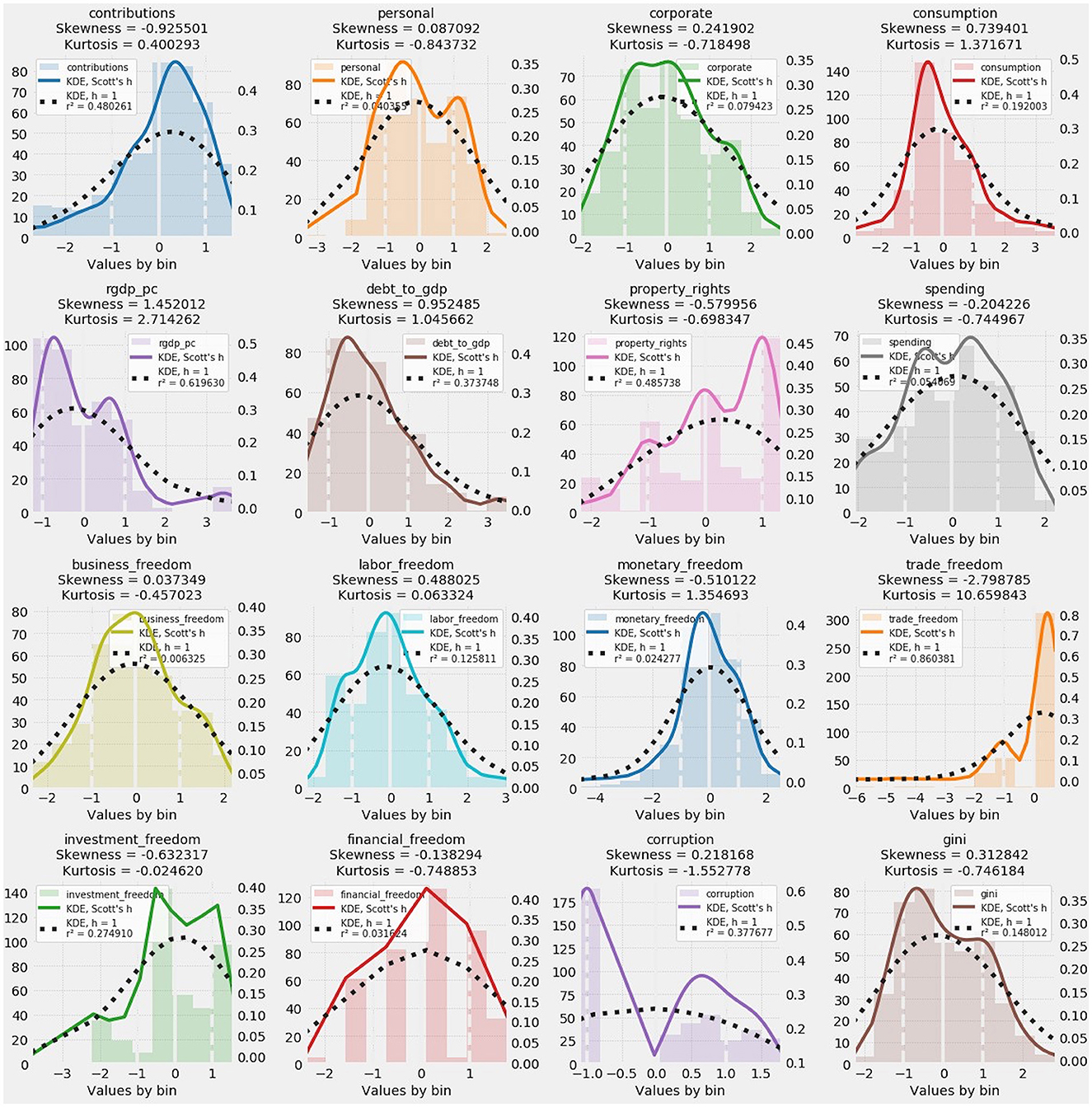
Figure 1. Histograms and kernel density estimates (KDEs) of predictive and target variables. Skewness and kurtosis for each variable are also reported. Departures from normality, wherever they occur, are readily visible in the histograms and KDEs as visual representations of the distribution of each variable.

The correlation matrix among these variables portrays the manageable level of correlation (Figure 2). No correlation is more extreme than ±0.700. Throughout this article, statistical significance is indicated as follows:

^*** p < 0.001

^** p < 0.01

^* p < 0.05

+ p < 0.10

Figure 2

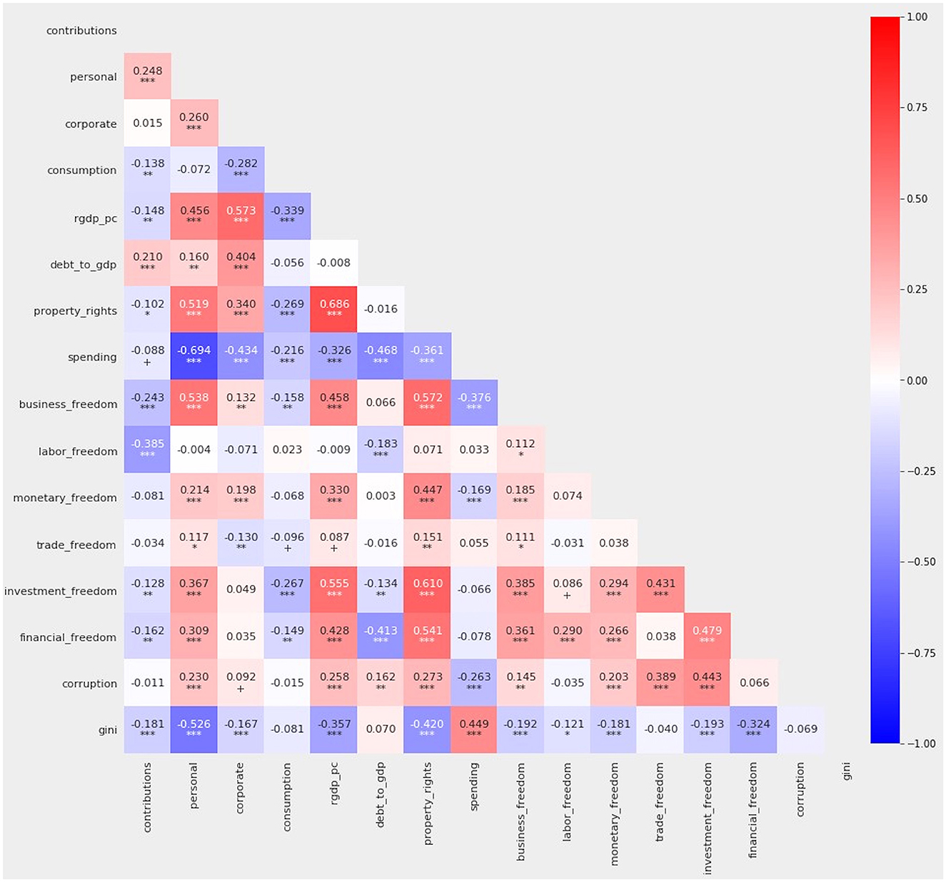
Figure 2. Correlation among all variables. Pearson's r is indicated on a sliding color scale where bright red indicates +1.000 and dark blue indicates −1.000.

This study's baseline model relies upon the ordinary least squares (OLS) regression of the foregoing predictive variables against the Gini coefficient:

$\begin{array}{ll}{y}_{it}={\beta }_0+x_{it}^{{}^{\prime }}\beta +{\epsilon }_{it}& (1)\end{array}$

where $x_{it}^{{}^{\prime }}$ is the array of independent variables, β is the vector of coefficients, and ε_it is the error term [32]. A simplification of the OLS model, omitting the _it subscript for entity- and time-specific instances, restates the specification as: $ŷ={\beta }_0+\sum _{i=1}^p{\beta }_i{x}_i+\epsilon ,x\in \left\{contributions,\dots ,corruption\right\}$. More elaborate specifications for advanced methods, which incorporate ℓ₂ and/or ℓ₁ penalties or fixed and/or random effects, appear in Sections 3.2 and 3.3.

We split data into randomized subsets for training and testing [[33], p. 17, 18]. Retaining test data helps generalize the model to data not seen during training. This study's training and test sets respectively comprise ¾ and ¼ of all data. The training set contains 303 records; the test set, 102.

To avoid leakage between training and test data, we applied Gaussian scaling drawn exclusively from training data [[33], p. 138–140]. Gaussian scaling yields beta coefficients [34], which can be evaluated without regard to the units in which raw variables are expressed [[35], p. 387]. The sign and scale of coefficients accompanying each predictor indicate the direction and strength of the impact on the target.

3.2 Regression methods and the no-free-lunch theorems

Especially in policymaking, regression serves two distinct purposes, corresponding to each side of the regression equation [[36], p. 702]. Some applications emphasize $\widehat{\beta }$, the vector of coefficients for explanatory variables on the right-hand side. Other applications focus on the fitted value of the response variable, y, on the left-hand side [[37], p. 1445]. Although this article emphasizes causal inference from $\widehat{\beta }$, it does use variability in predictive accuracy to evaluate the stability of causal inferences.

Causal inference among a set of predictors often requires selecting the correct subset of variables and assigning effect sizes reflecting either positive or negative impact on the response variable [38]. Type I errors through the mistaken inclusion of a predictor may arise [39]. Type II errors of omission also occur, if the design matrix fails to include a relevant variable [40, 41]. Null hypothesis significance testing—the analytical framework for an overwhelming majority of studies in economics and other social sciences—relies upon statistical conventions indicating the probability that a particular effect may have arisen by chance [42]. This study applies additional tools to strengthen the reliability of causal inferences regarding a highly complex socioeconomic phenomenon.

The no-free-lunch (NFL) theorems describe a pair of related propositions in mathematics and computer science, one for search [43] and the other for optimization through statistical inference [44]. In effect, the NFL theorems posit that there is no way to determine ex ante which mathematical tools will work best with a particular dataset for a particular task [45, 46]. The NFL theorems negate the notion that a fixed protocol can determine which methods will work best with a particular dataset and for the twofold goals of causal inference and predictive accuracy. Amid the inescapable uncertainty that bedevils efforts to evaluate large, complex collections of data, proper experimental design does not consist so much of a choice among specific methods, but rather a systematic application of all plausibly and potentially helpful methods, with an understanding of the rationales motivating the deployment of a particular methodological toolkit.

The inclusion of potential predictors in a design matrix is often—perhaps too often—constrained by the availability of data. It is entirely possible for a chosen set of predictors to be at once overinclusive and underinclusive. Regularized regression, broadly speaking, addresses the Type I error of injecting too many confounding variables into the design matrix. Fixed and random effects tests, by contrast, offer possible relief from omitted variable bias as a variant of Type II error in experimental design.

The proper focus therefore falls upon the goals of regression as a tool for interpreting a hypothesized model and estimating the effect of proposed predictors, as opposed to an unattainable set of a priori criteria for selecting specific regression methods. Some scientific applications, including this study, may be willing to sacrifice a degree of predictive accuracy for stability in experimental design and improved interpretability of a model. Among linear regression methods, any departure from OLS necessarily satisfies the optimal fitting of a predictive model, in the hope of improving the model's generalizability to new data.

Conscious departures from OLS may be informed by broad intuitions about families of advanced regression methods. Beyond coarse choices between regularization (on one hand) and fixed and random effects (on the other hand), the application of specific regression methods may hinge upon finer distinctions. Some specific choices may be guided by formal statistical tests such as the Hausman test. Distinct implementations of the ℓ₁ penalty have different tendencies to induce sparsity. In stacking generalization, the choice among supervised machine-learning methods might hinge on differences in the resilience of decision tree ensembles. Unsurprisingly, the mathematical clarity of methodological choices informed by formal tests or mere intuitions tends to decline as reliance on stochastic machine learning increases. Further details will emerge in this article's discussion of specific methods.

3.3 Regularized regression

To strengthen the credibility of its interpretive conclusions, this article deploys two distinct sets of advanced regression methods. The first of these departures from OLS is regularized regression. The second departure involves fixed and random effects regression. Each set of methods addresses a distinct obstacle to the proper interpretation of regression models.

First, collinearity may arise from irrelevant or redundant variables. When variables are collinear, one of those variables can draw an extremely large positive coefficient, only to be offset by a comparably large negative coefficient on another variable. These coefficients are unreliable, perhaps even misleading. Neither their size nor even their sign can be trusted [47].

The variance inflation factor (VIF) is often used to detect collinearity [48]. VIF > 10 [49] or even VIF > 5 raises cause for concern [[50], p. 119]. The VIF target is fluid because collinearity becomes less confounding as the amount of data increases [[51], p. 32].

Variable inflation factor analysis shows mostly acceptable values, with at most marginal cause for concern (Figure 3). No VIF value exceeds 5. Only four variables exhibit VIF values >3: personal (4.100), rgdp_pc (3.770), property_rights (3.331), and spending (4.724). Even mild collinearity, at VIF as low as 2.5, portends “difficulty in separating out the contribution of (affected) variables” [[52], p. 1958, 1959].

Figure 3

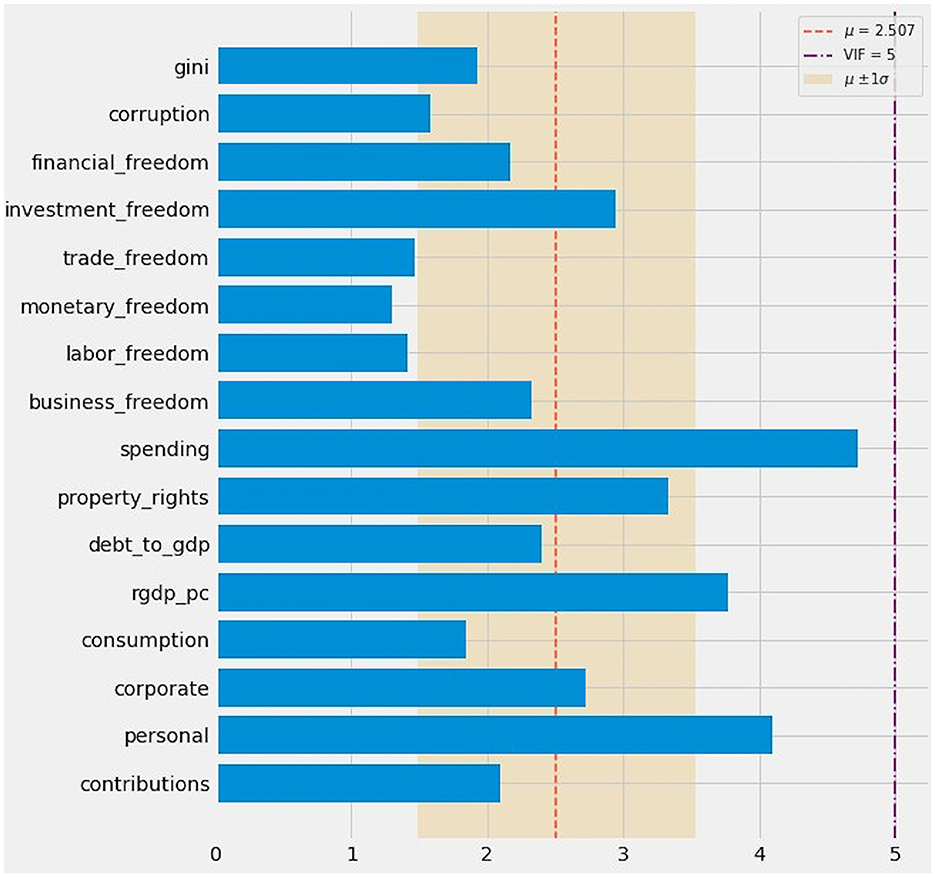
Figure 3. Variable inflation factor (VIF) analysis. Most VIF values fell below the conservative threshold of 2.5. All VIF values fell below 5.

Penalized (or regularized) regression methods can ameliorate collinearity. Ridge applies the ℓ₂ penalty to linear regression [53–56].

Ridge is most readily understood by its departure from OLS. OLS projects an n×1 column vector y onto n×p design matrix X. Multiplying the columns by the vector of coefficients, β ∈ ℝ^p×1, produces the projection Xβ. The estimator of β is:

$\begin{array}{ll}\widehat{\beta }={(X^{T}X)}^{-1}{X}^{T}y& (2)\end{array}$

Ridge regression adds a “ridge” named for the diagonal of the p × p identity matrix I_p:

$\begin{array}{ll}{\widehat{\beta }}_{Ridge}={(X^{T}X+\alpha I_p)}^{-1}{X}^{T}y& (3)\end{array}$

Ridge's penalization parameter, α ≥ 0, controls the degree of regularization. At α = 0, Ridge is equivalent to OLS. Increasing α raises the ℓ₂ penalty and redistributes weights within ${\widehat{\beta }}_{Ridge}$ toward zero relative to the least-squares estimate [[57], p. 237].

Regularization incorporating a ℓ₁ penalty can induce sparsity by assigning zero weight to inconsequential variables [38, 58]. Feature selection through sparsity removes irrelevant variables without excessive loss of information [59]. It also deletes otherwise relevant features rendered redundant by collinearity [60].

In principle, the induction of sparsity is the ideal method for removing irrelevant or redundant variables. Assigning zero weight unequivocally removes these variables from the design matrix and identifies an unambiguously active subset of predictors. At a minimum, however, all forms of regularized regression can shrink parameters. The shrinkage of parameters, paired with larger standard errors, tends to elevate p-values. Therefore, even in the absence of sparsity—an unavoidable attribute of Ridge parameters, which can be driven toward zero but never to zero—all regularized regression methods can work together with the apparatus of null hypothesis significance testing.

An efficient method for inducing sparsity exploits the least absolute shrinkage and selection operator, or Lasso [61–63]. The Lasso parameter λ adjusts the ℓ₁ penalty, specified as $\sum _1^p\left|{\beta }_j\right|$ [[64], p. 68, 69].

A hybrid of the ℓ₁ and ℓ₂ norms, ElasticNet combines the effects of Ridge and Lasso [65]. Like Lasso, ElasticNet can simultaneously shrink coefficients and select variables by inducing sparsity. ElasticNet tends either to include or to remove entire groups of highly correlated variables. Again, ceteris paribus, sparsity delivers clearer answers with respect to causal inference. Paradoxically, ElasticNet as a hybrid method incorporating an ℓ₂ penalty alongside an ℓ₁ penalty can be more efficient in inducing zero-weight coefficients. Surprises such as these, once again, demonstrate the no-free-lunch theorems and the futility of ex ante efforts to steer regularized regression methods according to the understandable but perhaps unattainable preference for sparse solutions over a merely shrunken set of parameters.

Sparse Bayesian learning can also generate zero-weight coefficients [66]. This trait invites the synonym, Bayesian Lasso [67]. SciKit-Learn adopts the name of the broader family of sparse Bayesian methods, automatic relevance determination (ARD).

Ridge, Lasso, ElasticNet, and ARD are machine-assisted regression methods. Cross-validation, which uses iterative resampling from different portions of training data to achieve out-of-sample testing [68], can set penalization parameters in Ridge [69], Lasso [70], and ElasticNet [[71], p. 3]. ARD uses Bayesian optimization of the ℓ₁ penalty as a “relevance vector machine” [66].

This study implemented automated, cross-validated versions of regularized regression in the SciKit-Learn library for Python. By default, that library cross-validates Ridge through the leave-one-out method. SciKit-Learn uses k-fold cross-validation, k = 5, for Lasso and ElasticNet. ARD in SciKit-Learn is a fully automated Bayesian method. This study coerced each regression method to find a zero intercept. In the interest of stability, this study raised the maximum number of iterations for Lasso and ElasticNet from 1,000 to 10,000. This study set the range of Ridge α as 150 (common) logarithmic intervals between 10⁻² and 10⁴ and the range of the ℓ₁ ratio in ElasticNet at 11 arithmetic intervals between 0.05² (0.0025) and 0.95² (0.9025). In all instances requiring a seed for Python's random number generator, this study used a seed of 1.

3.4 Fixed and random effects

Whereas collinearity typically arises from the overinclusion of variables, the opposite problem of under inclusion also vexes causal inference. The failure to identify an otherwise relevant, non-redundant variable can produce omitted variable bias [40, 41]. The coefficient of an omitted determinant of the dependent variable is non-zero. The covariance of an omitted variable z with specified independent variable x is also no-nzero: cov(z, x) ≠ 0. Fixed effects regression [72, 73], particularly the inclusion of time-invariant, country-specific effects [[13], p. 871, 872], can eliminate one source of omitted variable bias.

Since this dataset consists of 15 yearly observations for 27 countries, this study sought to neutralize omitted variable bias by deploying entity-, time-, and entity-and-time-based variants of a fixed effects model. The balance of this article will refer to these models as FEE, FTE, and FETE.

The FEE model may be written as:

$\begin{array}{ll}{y}_{it}={\alpha }_i+x_{it}^{{}^{\prime }}\beta +{\epsilon }_{it},{\epsilon }_{it}~IID(0,{\sigma }_{\epsilon }^2)& (4)\end{array}$

where α_i represents entity-specific heterogeneity and ${\epsilon }_{it}~IID(0,{\sigma }_{\epsilon }^2)$ indicates that all x_it are independent of all ε_it [[32], p. 386–388; [74], p. 484–486]. Each fixed effect unit (whether a geographic entity or a year) adds a dummy variable. The FTE model may be written similarly, with γ_t substituting for α_i.

By extension, the FETE model would include both α_i and γ_t:

$\begin{array}{ll}{y}_{it}={\alpha }_i+{\gamma }_t+x_{it}^{\prime }\beta +{\epsilon }_{it},{\epsilon }_{it}~IID(0,{\sigma }_{\epsilon }^2)& (5)\end{array}$

The random effects (RE) model assumes that all factors affecting the dependent variable, but not included among independent variables, can be expressed by a random error term. By analogy to FEE, the RE model may be written as:

$\begin{array}{ll}{y}_{it}=\mu +{\alpha }_i+x_{it}^{\prime }\beta +{\epsilon }_{it},{\epsilon }_{it}~IID(0,{\sigma }_{\epsilon }^2),{\alpha }_i~IID(0,{\sigma }_{\epsilon }^2)& (6)\end{array}$

where α_i + ε_it represents an error term containing a time-invariant specific component and a remainder component, presumably uncorrelated over time. In addition to being mutually independent, each component is also independent of x_it for all I and all t [[32], p. 347].

As applied to this dataset, the Hausman test [[75], p. 27, [76], 1251, 1252, [77, 78], 747] reports a result of χ² = 8.380128 at 15 degrees of freedom. The Hausman test begins with the null hypothesis that exogenous variables in the model are not correlated with omitted country- or time-specific attributes [[79], p. 123]. The p-value of 0.907641 associated with the Hausman test favors retention of the null hypothesis at any conventional threshold of statistical significance and adoption of the more efficient random effects model over a fixed effects model [[76], p. 1251, 1252].

Although the Hausman test favors random over fixed effects, other sources advise using both fixed and random effects when panel data covers a defined number of countries over a defined time period [[74], p. 495, 496]. Fixed effects may avoid potential biases arising in random effects from correlations between predictive variables and omitted attributes of each country [[80], p. 2771].

3.5 Stacking generalization

In order to aggregate predictions and inferences from nine linear regression methods, this article uses stacking generalization. This machine-learning method aggregates predictions from other models into a set of meta-predictions [81, 82]. Stacking generalization delivers “super learning” in high-stakes applications such as motion detection [83, 84].

Like all other machine learning ensembles [85, 86], a stacking model gracefully accommodates weaker methods. Thanks to this Delphic accumulation of learning from diverse sources, stacking can produce predictions more accurate than any of its tributary methods. Amid the profusion of advanced linear methods, stacking generalization can also produce an ex post sense of methodological order that cannot be attained until each of these underlying methods is applied and completes its work. In other words, meta-inferences generated by stacking generalization rationalizes the relative contributions of individual methods whose value to a study, according to the no-free-lunch theorems, cannot be predicted in advance.

This meta-ensemble stacks predictions from the nine linear methods as “level 0” in a new predictive model. Instead of the 15 features in the original dataset, stacking treats each distinct method in level 0 as an independent variable. A meta-learner, or blender, then enters the stacking model as level 1. After learning from training set predictions in level 0, the trained blender can produce its own predictions.

The level 1 blender can apply any regression method, linear or otherwise. This study devised its own stacking model to accommodate fixed and random effects regression, which relies on larger design matrices. This custom-built stacking generalization model can use a decision-tree ensemble such as random forests [87, 88]. Instead of searching for the best feature when splitting a node, random forests search for the best feature within a random subset. Randomizing thresholds for each feature, as opposed to searching for the optimal threshold, yields the extremely random trees algorithm, or extra trees [89].

Both random forests and extra trees, as ensemble-based methods of supervised machine learning, must be calibrated through cross-validation. Consistent with its reliance on default settings for the automatic cross-validation of Lasso and ElasticNet, this study manually implemented k-fold cross-validation, at a value of k = 5, for the random forest-powered and extra trees-powered stacking blenders. Again, Python's random number generator was seeded with the integer 1. Each stacking blender was calibrated so that each constituent decision tree would have a maximum depth of seven and no more than eight features.

The extra trees-powered blender delivered superlative accuracy. Relative to random forests, extra trees ensembles are more resistant to overfitting. This resilience arises from randomization of the subset of features and the point at which to split each tree within the ensemble [[90], p. 645, [91], p. 5].

The sum of a stacking blender's vector of feature importances is invariably 1. That vector may therefore be interpreted as the probability that a method in level 0 influences any prediction by the blender. Let the 15 × 9 matrix C represent all coefficients for the 15 predictive variables generated by the nine predictive methods. A 9 × 1 vector, called F, represents each of the feature importances in the stacking blender. The product of the matrix of coefficients and the vector of feature importances, C ·F, yields a new 15 × 1 vector V corresponding to the original 15 independent variables.

4 Results

4.1 The OLS baseline

The baseline OLS model ascribes a statistically significant relationship (at conventional thresholds of p < 0.10 or less) between the Gini coefficient and 12 out of 15 predictors (Figure 4).

Figure 4

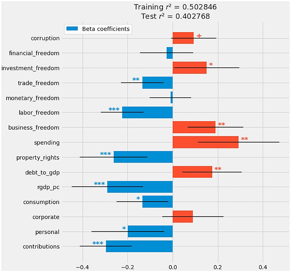
Figure 4. OLS regression: Beta coefficients, confidence intervals, and statistical significance. Indications of statistical significance follow the conventions described in Part 3.1.

The only predictors lacking significance at even p < 0.10 were corporate, monetary_freedom, and financial_freedom. Three out of four forms of taxation—social contributions, personal income taxes, and consumption taxes—exhibit a negative relationship with inequality. The higher the levels of these forms of taxation, the less unequal the distribution of income. Corporate taxation reported a weakly positive but statistically insignificant relationship with inequality.

The two macroeconomic features pointed in opposite directions. Real GDP per capita has one of the strongest negative effects on inequality. Larger European economies tend to be less unequal. By contrast, the higher the ratio of public debt to GDP, the more unequal the country's distribution of income.

Among the eight Heritage Foundation index components, the impact on inequality is roughly divided. Property rights, labor freedom, and trade freedom are all associated with reductions in inequality. Government spending, business freedom, and investment freedom point toward greater inequality. The relationship between inequality, on one hand, and monetary or financial freedom is negligible. Perceptions of corruption have a mildly positive relationship with inequality.

4.2 Regularized regression: Ridge, Lasso, ElasticNet, and ARD

Figure 5 reports coefficients and p-values for this study's nine linear regression methods as well as the composite model emerging from stacking generalization.

Figure 5

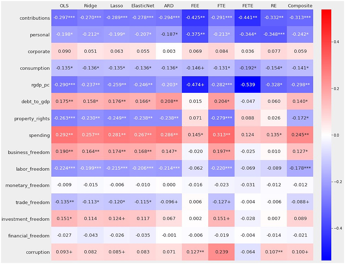
Figure 5. Coefficients and their statistical significance for nine linear methods and a composite drawn from an extra trees-powered stacking blender.

Despite mild collinearity, regularized regression did not induce (much) sparsity or discernibly shrink coefficients. The ℓ₂ penalty, α = 16.652388, did not materially distinguish Ridge from OLS. Ridge did deprive two variables, investment_freedom and corruption, of statistical significance. In light of misgivings over p-values [92] and the larger apparatus of null hypothesis significance testing [93], minor realignments within the conventional constellation of “significance stars” may justifiably be discounted or even ignored.

Two of the three methods incorporating an ℓ₁ penalty – Lasso and ElasticNet —failed to induce any sparsity. ARD assigned a zero coefficient to monetary_freedom and drove coefficients on corporate and financial_freedom nearly to zero. Among regularized methods, ARD achieved the greatest reduction in the absolute values of coefficients relative to OLS (Table 1).

Table 1

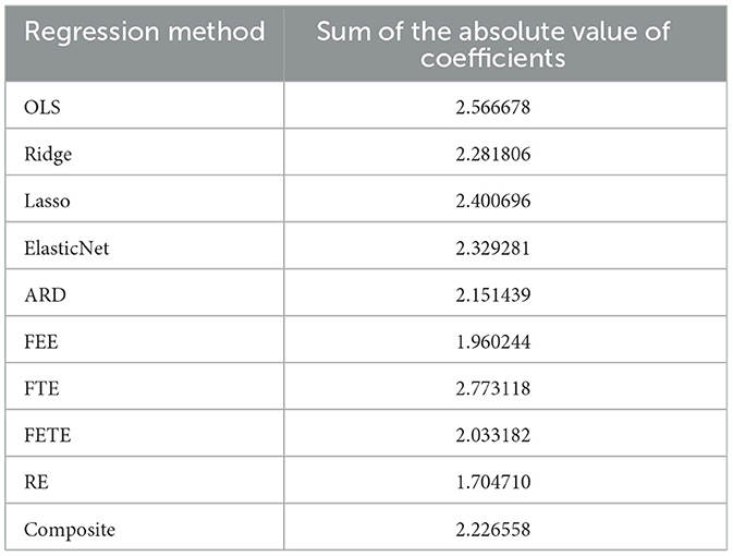
Table 1. The sum of the absolute value of coefficients generated by each regression method provides a crude indicator of each method's reduction or increase in the effect sizes reported by the baseline OLS model.

4.3 Fixed and random effects

Fixed and random effects regression also temper causal inferences drawn from OLS, but for reasons wholly distinct from those justifying regularization. Indeed, these two classes of regression methods have diametrically opposed motivations. Whereas Ridge, Lasso, ElasticNet, and ARD constrain collinearity among a possible surfeit of predictors, fixed and random effects remedy the possible omission of relevant, non-redundant variables.

This subsection first reports parameter estimates for FEE, FTE, FETE, and RE. These methods' fitted coefficients can and should be compared with those generated by OLS and regularized regression. This subsection then discusses entity- and time-specific effects, the most distinctive contributions of fixed effects methodology.

4.3.1 Parameter estimates for FEE, FTE, FETE, and RE

Among fixed and random effects models, fixed time effects (FTE) come closest to the OLS baseline. The close resemblance between OLS and FTE implies that annual differences from 2005 to 2019 do not materially affect predicted values of the Gini coefficient or the inference of causal relationships.

If anything, FTE amplifies effect sizes reported by OLS. Indeed, FTE is the only method to increase effect sizes relative to OLS. The absolute value of an FTE coefficient is often larger than that of its corresponding OLS coefficient. The most salient and intriguing instance involves FTE's treatment of corruption. FTE's estimate for corruption is nearly 2.6 times as large as the corresponding OLS coefficient. But FTE deprives that variable of statistical significance, because standard errors for corruption exceed the effect size by a multiple of nearly 2.4, and the p-value is 0.676.

The inclusion of fixed entity effects, whether in FEE or FETE, dramatically shifts the alignment of causal relationships among the 15 predictors. Two of the tax-specific predictors, contributions and personal, have much higher effect sizes relative to their corresponding coefficients under OLS and the regularized methods. FEE and FETE also deepened the negative coefficient for rgdp_pc.

Even more dramatically, FEE and FETE collapsed effect sizes for debt_to_gdp and all components of the Heritage Foundation index. Only spending retains statistical significance, and only under FEE. FETE reverses the sign on the coefficients for debt_to_gdp, business_freedom, and investment_freedom. All of these variables, identified by other methods as exacerbating income inequality, bear negative coefficients under FETE. Relative to OLS, the regularized methods, and FTE, FEE also flips business_freedom from positive to negative. Extreme shrinkage in effect sizes, to say nothing of a reversal of the sign, undermines causal inferences otherwise attributable to these variables.

Recall that the Hausman test prefers random over fixed effects for this dataset. These disparate treatments of potentially omitted variables are ultimately compatible. RE results are most closely aligned with FEE or FETE. Any difference between fixed and random effects proves inconsequential. The convergence of results for random and fixed effects vindicates recommendations that both of these tests be applied to panel data containing both intertemporal and geographic diversity [[74], p. 495, 496].

Like tests incorporating fixed entity effects, random effects deepen the association between higher levels of taxation (except corporate taxes) and lower income inequality. Relative to OLS, RE attributes a greater effect size to contributions, personal, consumption, and rgdp_pc. For all of these variables, RE is less exuberant than FEE and FETE. RE matches FEE and FETE in denying statistically significance to the debt-to-GDP ratio and all Heritage Foundation variables except spending. Confusingly enough, RE agrees with OLS and FEE in assigning a positive and statistically significant coefficient to corruption. FETE remains the lone method to attribute a negative (but insignificant) relationship between corruption and the Gini coefficient.

A review of Table 1, which reports the sum of the absolute value of coefficients in each model, heightens these comparisons of fixed and random effects with OLS and regularized regression. Intriguingly, RE assigns by far the most conservative vector of coefficients, as measured by the sum of their absolute value.

The sum of absolute values of coefficients is also lower for FEE and FETE relative to the regularized methods. This phenomenon can be attributed to the presence in fixed effects tests of 27 or 42 dummy variables, accounting (respectively) for the 27 EU member-states or those 27 countries plus the 15 years in this dataset. FTE, by contrast, has the highest sum of absolute values. Fixed time effects do not redirect values away from the coefficients assigned to core variables.

By conventional measures of statistical significance, FETE is even more conservative than random effects. FETE recognizes only three significant variables: contributions, personal, and consumption. All of those variables represent levels of taxation, and all three show a negative effect on the Gini coefficient. Remarkably, FETE assigns a coefficient of −0.539 to rgdp_pc, the largest effect size in this study, even as it deprives that variable of statistical significance. Again, this is an artifact of standard errors; the p-value for rgdp_pc in FETE is approximately 0.135—relatively low, but not low enough to satisfy any conventional p-value threshold.

4.3.2 Entity- and time-specific effects

FEE and FETE generated their own estimates of entity-specific effects. The subplot at left in Figure 6 shows each method's estimates and the similarity between the two sets of estimates. Even more helpfully, entity-specific effects correlate with the Gini coefficient for each member-state of the EU. For FEE alone, r = 0.517788. Because FETE produces a poorer fit with Gini, the average of entity-specific effects for FEE and FETE lowers r to 0.478948.

Figure 6

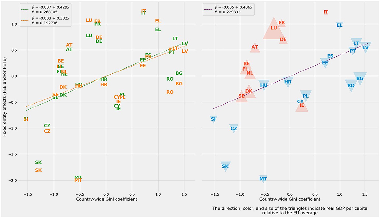
Figure 6. At left: Fixed entity effects plotted against Gini coefficient averages for each member-state of the European Union. FEE appears in green; FTE, in orange. At right: Combined fixed entity effects as the average of FEE and FETE, plotted against national Gini coefficient averages. The direction, color, and size of the triangles indicate real GDP per capita relative to the EU average.

A simple visualization of the relationship between (1) the average FEE and FETE parameter estimates for entity-specific effects and (2) the average Gini coefficient for each EU country demonstrates the basic soundness of these entity-specific estimates (Figure 6, right). Linear regression of country-wide Gini against the average of the FEE and FETE parameter estimates shows a positive slope (m = 0.406) and r² = 0.229392.

The two fixed-entity effects methods, FEE and FETE, provide additional information through country-specific parameter estimates. The combined subplot at right in Figure 6 adds triangles to each country. Red, upward-pointing triangles indicate higher-than-average real GDP per capita. Poorer countries are marked by blue, downward-pointing triangles. The size of each triangle indicates the degree of departure from the European mean.

The richer red cohort comprises all six of the founding members of the European Economic Community; the three Nordic states of Denmark, Sweden, and Finland; and Austria and Ireland. From the Treaty of Rome onward, many of these countries have had greater engagement in pan-European politics. The poorer blue cohort contains the extended Mediterranean group of Cyprus, Greece, Malta, Spain, and Portugal—a geographic swath evocative of the Odyssey, the Aeneid, or even the Punic Wars—plus every EU member-state that experienced a socialist frolic and detour after World War II.

The division between the richer, more equal countries in red and their poorer, less equal counterparts in blue may be imperfect, but it is evident and striking. By and large, the countries in red are the old member-states of the EU-14 (minus Portugal, Spain, and Greece). The countries in blue are mostly the new member-states of the EU-13.

Aside from two low-inequality outliers (Slovakia and Malta), poorer countries in blue tend to lie close to the regression line treating fixed entity effects as a function of the Gini coefficient. Fixed entity effects, however, tend to overestimate inequality in the richer red cohort. Ireland is a notable exception; entity effects underestimate Irish inequality.

On balance, fixed entity effects—including their errors in estimation—capture deeply historical differences within Europe. At their most effective, regression and related forms of supervised machine learning can perform tasks typically associated with classification and clustering. An examination of fixed entity effects, real GDP per capita as a surrogate for prosperity, and the ground truth of the Gini coefficient bifurcated Europe along historical, economic, and political differences.

By contrast, time-specific effects are more confounded. Though both contained a temporal element, the FTE and FETE methods assigned opposite effects to individual years from 2005 through 2019. Figure 7 plots FTE and FETE parameter estimates against Gini coefficients by year.

Figure 7

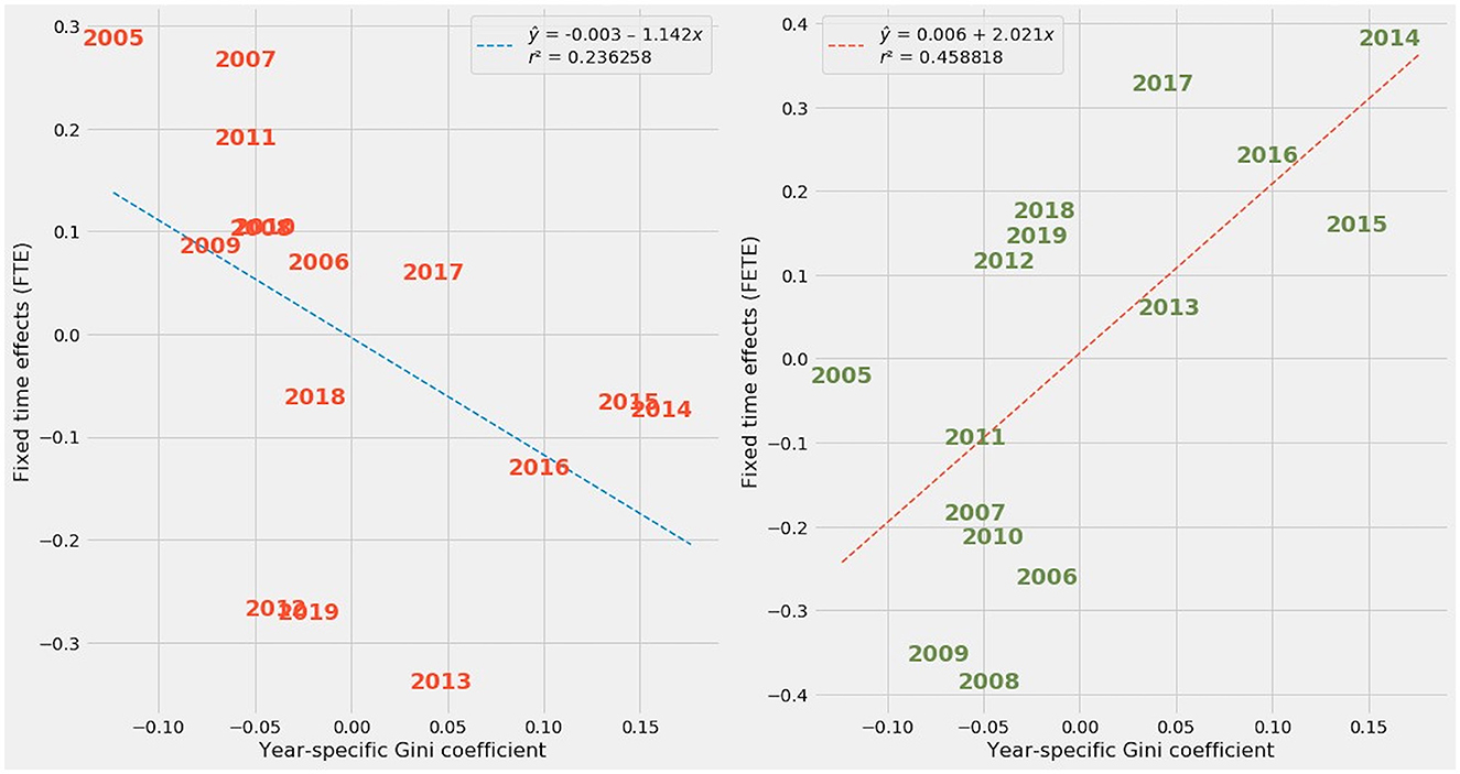
Figure 7. At left: Fixed time effects (FTE) plotted against year-specific Gini coefficient averages. At right: Fixed entity and time effects (FETE) plotted against year-specific Gini coefficient averages.

The regression line for FTE estimates of time-specific effects has a negative slope, while the regression line for FETE estimates slopes upward. The upward spike in year-by-year Gini coefficients after 2012 is readily apparent in FETE estimates. In truth, Gini coefficients trended upward from 2005 to 2019 in Europe (Figure 8) and elsewhere throughout the developed world [9].

Figure 8

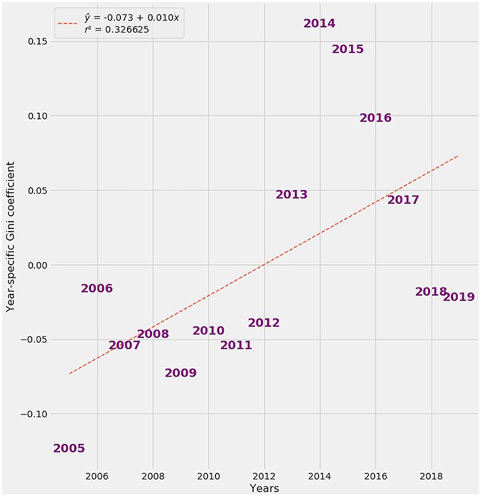
Figure 8. Year-specific Gini Coefficient averages as a function of actual years, 2005–19.

When contrasted with the upward trend in Gini coefficients, the downward slope in FTE's estimate of time effects reveals a misattribution of the relationship between time and economic inequality. FTE mistakenly implies that later years have lower inequality, when in reality the opposite happened.

Why, then, did FETE succeed in capturing the evolution over time of economic inequality while FTE failed? There may be unresolved collinearity between the FTE model's dummy variables for each of the years, on one hand, and the tax-based, macroeconomic, and nakedly political variables in the rest of the design matrix. Though not fully explored in this study, economic intuition suggests that autocorrelation and other time-series effects are embedded in factors such as the debt-to-GDP ratio or GDP per capita.

The same year-by-year dummy variables also appear in FETE. But the design matrices for OLS and the fixed effects methods differ radically in shape. Training data for all methods contained 303 observations, or roughly three-fourths of 405 total observations (27 countries over 15 years). OLS contains the same 15 basic predictors common to all models. FTE adds 15 dummies for the years. FETE adds another 27 dummies for EU member-states. The FTE design matrix therefore assumes a 303 × 30 shape, while FETE uses a 303 × 57 design matrix.

Ordinarily, collinearity compounds as the dimensionality of a design matrix increases. In this instance, however, the addition of 27 entity-specific dummies nearly doubles the number of predictors in FETE relative to FTE. Time-specific dummy variables, whatever their collinearity with the baseline economic predictors, evidently did not interact in a destructive way with the entity-specific dummies.

Put another way, the introduction of time-specific dummy variables in FTE may have exaggerated latent time-dependent traits in variables reflecting macroeconomic conditions, tax policy, and political ideology. As often happens amid excessive collinearity, FTE assigned arbitrary large coefficients to the time-specific dummies, pointing the opposite direction from those years' relationship with economic inequality.

By contrast, the introduction of 27 entity-specific dummies in FETE diluted the deleterious impact that time-specific effects may have had on collinearity. The stability of FEE and FETE reinforces confidence in the validity of entity-specific effects. Those models evidently capture something unique to the European Union's geographically, socially, and economically diverse member-states. True to the mission of fixed effects regression, entity-specific effects successfully identify factors missing from OLS and its regularized extensions.

4.4 Both sides now: the two faces of stacking generalization

Stacking generalization typically enhances predictive accuracy in supervised machine learning. But the insertion of an extra trees blender as the “level one” aggregator of the linear methods in level zero produces a vector of feature importances that assigns a probability that a particular method has influenced the blender's predictions. This vector therefore measures the contributions of methods, from OLS to regularized regression and fixed and random effects, to predictions made by the stacking blender. The weights attributed to each method in level zero produce a composite model whose coefficients, confidence intervals, and p-values can be compared to the conventional statistical apparatus of OLS and its advanced cognates.

This subsection reports each contribution of stacking generalization in turn. It first reports fitted values for all methods and the aggregation of those predictions through stacking generalization. This subsection then extracts a composite linear model from parameter estimates by all methods in level 0, as weighted by the feature importances of the extra trees blender in level 1.

4.4.1 Fitted values in ŷ and measures of predictive accuracy

Since most applications of stacking generalization strive for predictive accuracy, this subsection is the best place to present predictions from all methods. The grid of 12 subplots in Figure 9 presents ŷ, the vector of fitted values for all nine linear methods, from OLS to four regularized methods and the four fixed and random effects tests. It also includes three composite predictions: a soft voting regressor that aggregates Ridge, Lasso, ElasticNet, and ARD [94, 95], plus random forest and extra trees blenders.

Figure 9

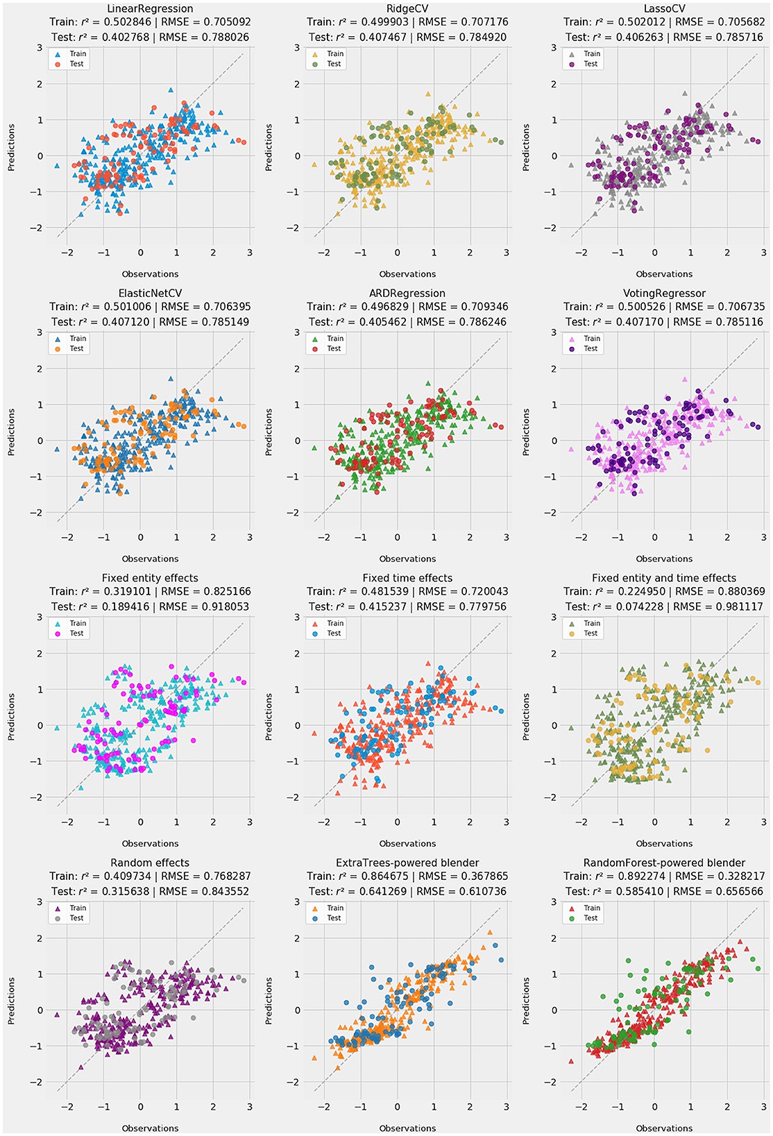
Figure 9. Twelve subplots depicting training and test-set predictions for all methods: OLS, regularized regression, fixed and random effects, and stacking blenders. Goodness-of-fit statistics [r² and root-mean-square error (RMSE)] are reported for training and testing subsets for each method.

Perhaps the most striking result is stacking generalization's improvement in accuracy. The extra trees blender outperforms random forests, but either blender is more accurate with respect to test data than even OLS in training. The extra trees blender is particularly impressive, with r² scores of 0.864675 in training and 0.641269 as applied to test data. Corresponding r² scores in OLS are 0.502846 and 0.402768.

Because of its “sometimes unintended and exasperatingly precise … results,” stacking generalization as a form of ensemble learning is said to bear “an uncanny resemblance to the Delphic Oracle in mythology” [[96], p. 11]. Machine learning based on a Delphic chorus of weak predictors can deliver more accurate results than a single, more elaborate predictor. As often happens in machine learning, this stacked ensemble outperformed its individual components. Indeed, predictive improvement is so stark that stacking generalization can be said to have revealed countervailing strengths among the constituent models. Again, regularization and fixed or random effects tests address different sources of bias. Accordingly, these distinct families of methods should be expected to yield diverse results on both sides of the regression equation.

Strong test set accuracy also demonstrates stability in stacking generalization and the credibility of the methods in level 0. Retaining three-quarters of the r² score in the transition between training and testing suggests that the stacking blender is doing more than merely fitting instances seen during training.

Predictive accuracy among methods in level 0 also warrants closer examination. Regularization and fixed and random effects are celebrated as weapons against collinearity and omitted variable bias on the right-hand side of the regression equation. Nevertheless, the retention or loss of accuracy with respect to test data reveals the stability and reliability of each method. OLS always outperforms regularized regression in training.

Every regularized method and the voting regressor aggregating Ridge, Lasso, ElasticNet, and ARD outperformed OLS on test data. This attribute of the predictions, however modest, validates resort to regularization. Despite the conscious sacrifice in training accuracy through an ℓ₂ and/or ℓ₁ penalty, regularized regression is more stable and generalizable than OLS. Regularization reduced variance without sacrificing predictive accuracy on new data.

Fixed and random effects varied in their predictive performance. Fixed and random effects should not be expected to be as robust against overfitting as regularized regression, since these methods affirmatively expand the design matrix. Methods incorporating fixed entity effects, FEE and FETE, slipped badly on test data. But FTE and random effects showed stability comparable to the regularized methods. RE's superior accuracy and stability vindicate the Hausman test, which recommended random over fixed effects for this dataset. For its part, FTE outperformed every other linear method on test data, attaining r² of 0.415237.

The superlative performance of FTE on test data, however, does not eliminate the possibility that the addition of time-specific effects elevated collinearity. Collinearity does not ordinarily impair predictive accuracy or the ability to fit a model to new data, as long as the predictors follow the same pattern of collinearity [[97], p. 369–70; [98], p. 283]. Sampling variability, however, does affect predictive accuracy as well as causal inference in collinear data. Declines in accuracy as between training and test data may therefore stem in part, though perhaps not substantially, from latent or introduced collinearity.

4.4.2 A composite linear model based on stacking blender feature importances

Gini impurity in the extra trees blender's predictions enables the attribution of feature importances to all of the methods in level 0. These feature importances are readily interpreted as the weight of each method's contribution to the stacking blender's meta-predictions (Figure 10).

Figure 10

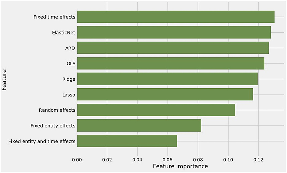
Figure 10. Feature importances among regression methods as reported by their Gini impurity within the extra-trees-powered stacking blender.

Contributions from the nine constituent methods are not equal. FTE generated the most accurate test set predictions. It received the highest weight in stacking generalization. OLS and the four regularized methods all received more than their expected weight. Aside from FTE, fixed and random effects methods received modestly less weight.

These weights help build a composite linear model. Parameter estimates can be straightforwardly multiplied by the extra trees blender's feature importances as a vector of weights. For instance, FTE received 0.130688 of the blender's importances. Multiplying that weight against all coefficients in $\widehat{{\beta }_{FTE}}$, FTE's fitted vector of coefficients, yields FTE's contribution to the composite. The same process is repeated for t-values for each predictive variable in each of the nine linear models. These composite t-values are readily transformed into standard errors (the ratio of the coefficient to the t-value) and p-values ($p=2·\left[1-CD{F}_{Studen{t}^{{}^{\prime }}sT}(\left|t\right|,df=287)\right]$).

The final composite model closely resembles OLS, with the same configuration of positive and negative coefficients (Figure 11). These coefficients also appear in the right-most column of Figure 5. The composite model deprives exactly one predictor of statistical significance: investment_freedom. Relative to OLS, the composite model does widen confidence intervals for most variables and, consequently, reduce the level at which 11 of 15 variables are considered statistically significant. But there is a consensus that corporate taxation, monetary_freedom, and financial_freedom are inconsequential.

Figure 11

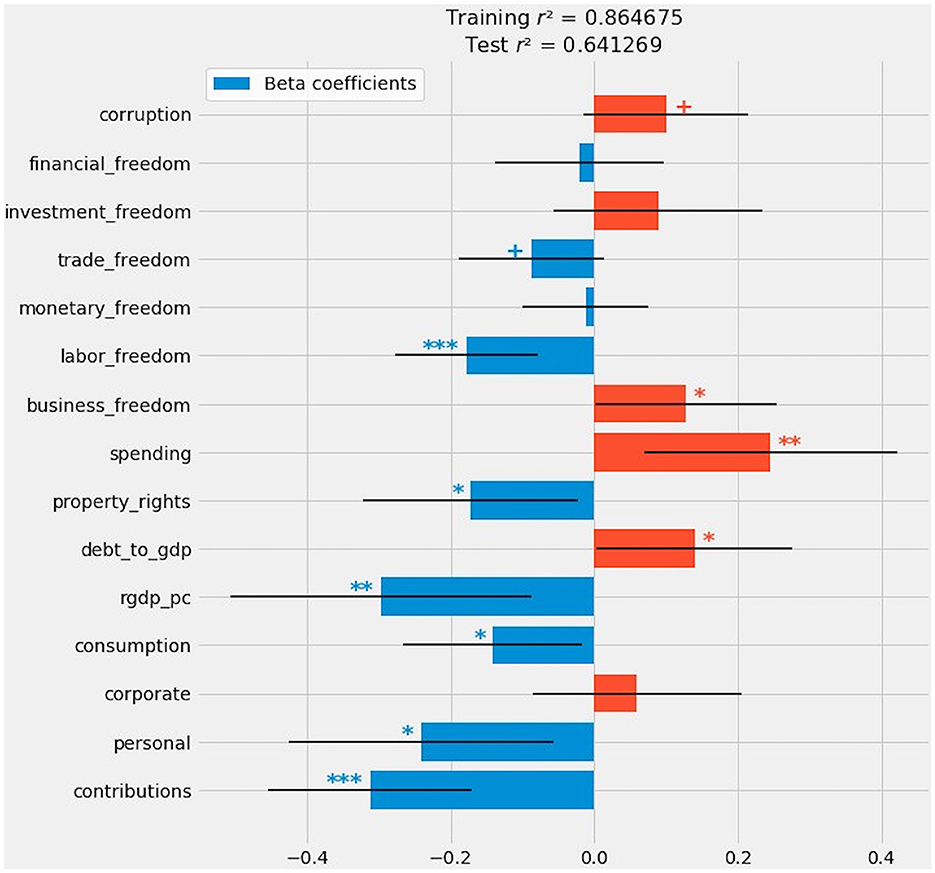
Figure 11. A composite of all generalized linear methods after stacking generalization: OLS, regularized regression, and fixed and random effects.

5 Discussion

The relationship between tax policy choices and income inequality demands extremely close and careful scrutiny. This study's results provide ample reason to doubt many of the causal inferences that might be superficially and prematurely drawn from OLS, any advanced linear method, or the stacked composite. Some or perhaps even many of the 11 variables emerging from stacking generalization's meta-analysis of weaker models may not survive deeper scrutiny.

5.1 The switching of signs on coefficients: fixed and random effects

Recall Figure 5's presentation of all parameter estimates and their statistical significance. Instability in the sign for each coefficient across all nine methods cautions against reflexive reliance on conventional indications of significance. If all nine methods rest on a credible basis, then even a single reversal in the sign of a coefficient undercuts causal inferences arising from the sign, size, and (if one insists) statistical significance of a coefficient.

Effect size matters more than arbitrary p-value cutoffs. The farther a coefficient lies from zero, the harder it will be to flip its sign. By contrast, a coefficient whose absolute value is lower, even if statistically significant at some conventional threshold, is more vulnerable to a change in sign.

Coefficients for these six variables reverse sign:

• The ratio of public debt to GDP (from positive to negative, relative to OLS)

• Property rights (negative to positive)

• Business freedom (positive to negative)

• Trade freedom (negative to positive)

• Investment freedom (positive to negative)

• Corruption (positive to negative)

In all but one of these instances, one of the methods incorporating fixed entity effects flips the sign. FETE flips five out of six (every one of these variables except trade_freedom). FEE reverses property_rights, business_freedom, and trade_freedom. Although FEE and FETE are the weakest predictive models, both of these fixed entity effects methods delivered credible entity-specific estimates for the 27 member-states of the European Union. The random effects test reversed the sign on property_rights, the flipped variable with the greatest effect size under OLS.

Almost all of these reversals in sign took place in fixed effects regression, specifically in models including fixed entity effects. The design matrices for FEE and FETE included 27 dummy variables for each of countries in the EU. These models did not have the most conservative parameter estimates as measured by the sum of the absolute value of coefficients (Table 1). Rather, FEE and FETE ranked between ARD (the most conservative of the regularized methods) and random effects, by far the most conservative method overall. Moreover, FEE and FETE redistributed some of their effect sizes to three of the tax-related variables (contributions, personal, and consumption) and to rgdp_pc. FEE and FETE evidently shifted effect sizes on public indebtedness, many of the Heritage Foundation index components, and corruption to decidedly non-zero entity-effect estimates.

5.2 The switching of signs on coefficients: Ridge path

The Ridge path provides a second, more mathematically rigorous basis for eliminating variables from the active set, or at least downgrading their credibility [99]. It is possible to test a wide variety of values for penalization parameters such as Ridge α. If a coefficient, across plausible values for α, changes its sign, its transit across zero undercuts its predictive validity and credibility.

The Ridge path flipped the signs on these four variables (Figure 12):

• corporate

• business_freedom

• investment_freedom

• corruption

Figure 12

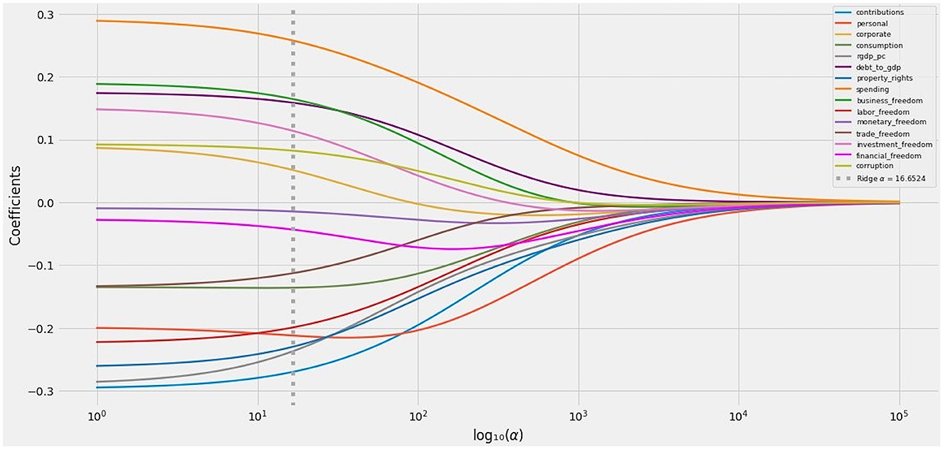
Figure 12. The Ridge path: Ridge coefficients as a function of regularization at values of α ∈ (10⁰, 10⁵).

Three of these variables, unsurprisingly, were among those whose coefficients flipped under FEE, FETE, or RE. The fourth, corporate taxation, is the only tax-specific variable that failed to attain statistical significance under any method.

The combined effect of an across-the-board evaluation of parameter estimates by all nine linear methods and a look at the Ridge path is to undermine trust in four out of 11 variables deemed statistically significant by the composite:

• debt_to_gdp

• property_rights

• business_freedom

• corruption

The variables that have not survived further scrutiny are the debt-to-GDP ratio, two components of the Heritage Foundation index, and corruption. These are variables that have received mixed treatment in literature evaluating drivers of income equality. Public indebtedness and corruption, in particular, are not associated with an unequivocal impact on inequality. Contested in the literature, these factors emerge from this study with mixed results.

Moreover, the finding that citizens of relatively unequal societies favor meritocratic accounts of inequality suggests that abstract notions of economic freedom, embraced or rejected in varying degrees across developed democracies, do not serve as universal, invariant drivers (in either direction) of income inequality. Though beliefs treating inequality as meritocratic suggest that voters in unequal societies may want that they get, after-the-fact rhetorical support for unequal outcomes does not necessarily imply that these voters get what they want. Post-hoc rationalization is an emotional salve, not evidence of the heart's true desire ex ante [100, 101].

5.3 An evaluation of surviving predictors

This study has used the totality of its data analysis and the Ridge path to supplement conventional thresholds of statistical significance. In concert, these tools winnowed out variables that might warrant closer attention under rigid adherence to statistical convention. Seven variables remain worthy of continued consideration:

• contributions (negative)

• personal (negative)

• consumption (negative)

• rgdp_pc (negative)

• spending (positive)

• labor_freedom (negative)

• trade_freedom (negative)

By contrast to ideological variables, tax-related variables (with the notable exception of corporate taxation) all have a statistically significant and negative impact on the Gini coefficient. Alongside real GDP per capita, a proxy for nationwide affluence, tax policy has the greatest impact on income inequality. More modestly, this study can conclude that tax policy appears to have a greater impact on inequality than ideological or behavioral indicators such as corruption or the Heritage Foundation's libertarian index of freedoms.

The two freedoms credibly related to inequality are associated with labor and trade. The emergent intuition is that freedom vis-à-vis international trade softens economic inequality. A similar inference arises with respect to the domestic labor market. Comparative advantage and the freedom to sell one's labor on favorable terms presumably reduce inequality. Both of these inferences contradict the conventional account that ascribes rising inequality to globalization and the widening gap in the earning potential of educated and uneducated workers. Atkinson's more optimistic view [6, 7] finds some support in the parameter estimates for labor and trade freedom.

The most intriguing variable may be spending. This variable has the highest positive effect on the Gini coefficient. Government spending, as the side of fiscal policy opposite taxation, apparently has the opposite and perhaps unexpected or counterintuitive effect relative to taxation. Whereas, taxation is generally associated with reductions in inequality, higher levels of spending are associated with more rather than less economic inequality.

There is some principled mathematical basis for doubting this causal inference. Spending has this study's highest variable inflation factor (Figure 3). It is palpably related to tax-based variables, since countries collecting higher taxes can spend more. It is also related to GDP per capita. Wealthier countries, ceteris paribus, spend more—privately and in the public sector. Those expenditures may advance policies that are more effective in reducing inequality, such as universal education and preventive health care, but less likely to be adopted in poorer countries. Even if conclusions regarding specific expenditures are elusive or premature, the literature does suggest that social spending is more effective in reducing inequality in richer countries.

Among other possible reasons for lower inequality in wealthier countries, the efficacy and efficiency of public-sector expenditures may contribute to the Kuznets curve. Even if the effect of wealth cannot be inferred from the opposite signs on spending and three tax-based variables, entity effects in FEE and FETE support Kuznets' hypothesis that inequality reverses its relationship to economic growth once a society reaches a critical turning point.

In order to alleviate collinearity, this study omitted two originally contemplated variables: the tax_burden and integrity components of the Heritage Foundation index. Tax_burden is manifestly collinear with the tax-specific variables of contributions, personal, corporate, and consumption. To a lesser extent, so is spending. The presence of a large and opposite-signed coefficient on spending, almost as a mirror image of the negative coefficients on contributions, personal, and consumption, raises legitimate concern that residual collinearity undermines this study's causal inferences.

On the other hand, there truly are meaningful differences between the revenue side of fiscal policy and the government's spending priorities. Omitting variables does not come free of epistemological cost. Mistakenly omitting a relevant variable, despite alleviating pressure on the variable inflation factor, may introduce specification bias [[97], p. 365, 366]. Moreover, both the omitted tax_burden variable and the retained spending variable are positively correlated with gini. In both instances, 0.44 < r < 0.45 (Figure 2).

It is entirely plausible that government spending can exacerbate income inequality, while three of four modes of taxation (all except corporate taxation) correspond with reductions in the Gini coefficient. This finding is consistent with commonplace economic wisdom that taxation is a more effective weapon against inequality than spending. Unless tax policy is aggressively or even maliciously regressive, the incidence of taxation falls more heavily on higher-income taxpayers. The resulting reduction in economic inequality is unambiguous.

By contrast, spending reduces inequality only if it effectively targets poorer recipients. There are ample reasons to doubt whether certain governments achieve or even intend any such thing. Governments are not known for effectively directing payments toward poorer recipients, even when they consciously seek to transfer wealth. Defense and health care expenditures notoriously evade the poor [102–104]. Evidence from poor countries (admittedly outside Europe) suggests that expenditures on infrastructure and basic services such as education and health care disproportionately benefit non-poor citizens [105, 106]. If spending favors more affluent citizens, it may aggravate economic inequality.

6 Conclusion

6.1 An overview of this study's conclusions

Economic policy and its implementation can affect both growth and inequality. Reductions in inequality will depend on policies and reforms implemented by the member-states of the European Union. Effective policy depends in turn on knowledge of the drivers of income inequality. This study has examined the impact of tax policies, indicators of economic freedom, and macroeconomic traits.

The tax system and social benefit programs are key instruments for redressing income inequality. Used appropriately, these measures can directly reduce inequality. These policy implications are stronger for the poorer countries of the “new” member-states of the EU-13. Even among countries in central and Eastern Europe, which share many historical and political commonalities, differences in tax policy and social spending yield divergent outcomes as between the Baltic states and the Visegrád countries of Hungary, Czechia, Slovakia, and Poland [107].

6.2 Methodological conclusions

This article has deployed a novel analytical apparatus to evaluate the relationship between tax policy, macroeconomic conditions, political attitudes, and income inequality. Each set of tools addressed a potential source of econometric bias or uncertainty.

Regularized regression did not appreciably change causal inferences drawn by baseline OLS. Modest collinearity remained under control and did not undermine the model's generalizability and reliability.

Fixed effects regression successfully identified country-specific effects not captured by the basic design matrix. FETE outperformed FTE in capturing time-specific effects. These advanced methods emphasized tax policies at the expense of the debt-to-GDP ratio and ideological factors. All models were consistent with the Kuznets curve hypothesis and with literature arguing that Europe (or at least its richer countries) has apparently crossed the turning point beyond which further economic growth reduces rather than increases inequality. Higher GDP per capita, ceteris paribus, should be expected to lower the Gini coefficient.

Diversity among regression methods strengthened the predictive power of stacking generalization. The extra trees blender improved test accuracy by roughly 0.25 in r². Feature importances within the blender assigned a weight to each linear method in level 0 and enabled the extraction of a composite model.

Although the composite did not appreciably differ from the OLS baseline, instability in parameter estimates across this article's full range of methods cast doubt upon causal inferences that might be upheld according to statistical convention. Fixed and random effects undermined the credibility of OLS and methods applying an ℓ₂ or ℓ₁ penalty. Variables that crossed zero along the Ridge path likewise invited analytical skepticism.

Tempered by these reservations, the composite model found that real GDP per capita and all forms of taxation except corporate taxes have a negative relationship with the Gini coefficient. Two Heritage Foundation index components—trade and labor freedom—also attracted parameter estimates suggesting a reduction in inequality. Perhaps counterintuitively but consistent with at least some of the literature, higher social spending is associated with affirmative increases in inequality.

6.3 Policy implications

This study's policy implications vary in their clarity. Three forms of taxation—social contributions, personal income taxes, and consumption taxes—are strongly connected with reductions in income inequality. These findings reinforce conventional trust in progressive taxation as the most effective instrument against inequality. The case for universal basic income and other social transfers is more ambiguous. Spending appears to exacerbate inequality. No other factor compounding inequality has a higher effect size, and other hypothesized aggravators of inequality did not survive closer analytical scrutiny.

By the same token, this study gives at best qualified support for the proposition that a high ratio of debt to GDP worsens income inequality. Though OLS and regularized regression support this inference, fixed and random effects disagree. Challenges posed by growing inequality squarely enter the debate over the relationship between government debt and economic growth. Whether Reinhart and Rogoff [108] correctly identified public debt as a barrier to growth is one of the most thoroughly contested propositions in contemporary economics [109–111].

On one hand, public borrowing can stimulate investments with positive externalities throughout the economy. Stimulus spending can also alleviate economic downturns. On the other hand, elevated public debt crowds out private actors from credit markets and raises the long-term cost of borrowing.

Prosperity, as measured by real GDP per capita, has a negative effect on the Gini coefficient. This finding is consistent with the literature on the Kuznets curve. If lower-income countries have passed the turning point on the Kuznets curve, growth-enhancing fiscal and monetary policies may reduce inequality. These questions are impossible to extricate from the broader debate over debt and growth.

Among the ideological factors in the Heritage Foundation's index, trade and labor freedom appear to alleviate inequality. As a rule, these index components have lower effect sizes and more ambiguous support than tax-related factors and GDP per capita. Previous research reached contradictory conclusions about corruption. This study likewise found a possible positive relationship between perceptions of corruption and the Gini coefficient, but also ample reason to doubt this conclusion.

6.4 Future work

These conclusions guide future work. The most obvious extension would apply this study's experimental design beyond Europe. Economic, social, and political differences within Europe, though substantial, would be magnified in a global sample. Greater diversity within a worldwide dataset should highlight the methodological contributions of all the tools deployed in this study: regularization, fixed and random effects, and stacking generalization.

Other methodological extensions await. The first step may consist of applying other generalized linear methods. The prevalence of quadratic relationships throughout this branch of economics invites the application of polynomial regression. Although that method is canonically associated with overfit models [[112], p. 2–4], regularized regression tempers that concern. Quadratic regression may sharpen understanding of the Kuznets curve and its relationship to tax policy. Because the Laffer curve assumes a very similar shape, a quadratic model may add helpful nuance as scholars and politicians seek the optimal, revenue-maximizing level of taxation [113, 114].

A statistical apparatus for evaluating interaction effects is the natural byproduct of polynomial regression [115]. That class of effects describes the impact of prosperity (as measured by real GDP per capita) on the most confounded variables in this study: social spending, the debt-to-GDP ratio, and corruption. The presence of data on differences in real GDP per capita among European countries also invites an effort to decompose inequality into the between-countries and within-countries component of the Theil index.

This study applied stacking generalization strictly to linear models. Future work can use more computationally intense methods involving decision tree ensembles and/or support vector machines. Supervised machine learning can evaluate datasets curated for linear methods. Although supervised machine learning methods lack the interpretive clarity of linear regression, they do generate feature importances. Imperfect though the comparison may be, supervised machine learning can be evaluated alongside linear methods.

Unsupervised machine learning, particularly through clustering and manifold learning, may identify economically distinct subgroups among the member-states of the European Union. Entity effects and errors in their estimation have already revealed categorical differences within Europe. Future research should quantify differences among countries as well as inequality within them.

Data availability statement

The original contributions presented in the study are included in the article/Supplementary material. Further inquiries can be directed to the corresponding author.

Author contributions

JC: Conceptualization, Formal analysis, Investigation, Methodology, Project administration, Software, Supervision, Validation, Visualization, Writing—original draft, Writing—review & editing. NŠ: Conceptualization, Data curation, Investigation, Writing—original draft, Writing—review & editing. MS: Conceptualization, Funding acquisition, Investigation, Writing—review & editing.

Funding

The author(s) declare financial support was received for the research, authorship, and/or publication of this article. This research is based upon work from COST Action 19130 Fintech and Artificial Intelligence in Finance, supported by COST (European Cooperation in Science and Technology) www.cost.eu.

Acknowledgments

Charalampos Agiropoulos provided useful comments, especially with respect to fixed and random effects regression methods.

Conflict of interest

The authors declare that the research was conducted in the absence of any commercial or financial relationships that could be construed as a potential conflict of interest.

Publisher's note

All claims expressed in this article are solely those of the authors and do not necessarily represent those of their affiliated organizations, or those of the publisher, the editors and the reviewers. Any product that may be evaluated in this article, or claim that may be made by its manufacturer, is not guaranteed or endorsed by the publisher.

Supplementary material

The Supplementary Material for this article can be found online at: https://www.frontiersin.org/articles/10.3389/fams.2023.1282975/full#supplementary-material

Data Sheet 1. Raw data.

Data Sheet 2. Gaussian-scaled training data.

Data Sheet 3. Gaussian-scaled test data.

Data Sheet 4. Gaussian-scaled data, combining all training and test data into a single set labeled according to a five character code indicating the country and the year of each observation (e.g., AT_05 indicates Austria in 2005).

References

1. Stiglitz J. The Price of Inequality: How Today′s Divided Society Endangers our Future. New York, NY: W.W. Norton (2012) 560.

Google Scholar

2. Krueger AB. The Rise and Consequences of Inequality in the United States. Washington, DC: Council of Economic Advisers (2012).

Google Scholar

3. Greenstone M, Looney M, Patashnik J, Yu M. Thirteen Economic Facts about Social Mobility and the Role of Education. The Hamilton Project Policy Memo. Washington, DC: The Brookings Institution (2013).

Google Scholar

4. Kierzenkowski R, Koske I. Less income inequality and more growth – are they compatible? Part 8 the drivers of labour income inequality – a literature review. OECD Econ Department Working Papers. (2012) 931:1–31.

Google Scholar

5. Milanovic B. Global Inequality: A New Approach for the Age of Globalization. Cambridge, MA: Harvard University Press (2016), 320. doi: 10.4159/9780674969797

Crossref Full Text | Google Scholar

6. Atkinson AB. Can we reduce income inequality in OECD countries? Empirica. (2015) 42:211–23. doi: 10.1007/s10663-015-9288-0

Crossref Full Text | Google Scholar

7. Atkinson AB. Inequality: What Can Be Done? Cambridge, MA: Harvard University Press (2015), 400.

Google Scholar

8. OECD. Growing Unequal? Income Distribution and Poverty in OECD Countries. Paris: OECD Publishing (2008), 312.

Google Scholar

9. OECD. In It Together: Why Less Inequality Benefits All. Paris: OECD Publishing (2015), 336.

Google Scholar

10. Petzina D, Stolper WF, Hudson M. The Origin of the European Coal and Steel Community: Economic forces and political interests. J Inst Theor Econ. (1981) 137:450–68.

Google Scholar

11. Schmidt G. Die Römischen Verträge und der Ost-West-Konflikt. In:M Gehler, , editor. From the Common Market to European Union Building: 50 years of the Rome Treaties, 1957–2007. Vienna: Böhlau (2009), 85–109.

Google Scholar

12. Kuznets S. Economic growth and income inequality. Am Econ Rev. (1955) 45:1–28.

Google Scholar

13. Forbes KJ. A reassessment of the relationship between inequality and growth. Am Econ Rev. (2000) 90:869–87. doi: 10.1257/aer.90.4.869

Crossref Full Text | Google Scholar

14. Baiardi D, Morana C. Financial development and income distribution inequality in the euro area. Econ Model. (2018) 70:40–55. doi: 10.1016/j.econmod.2017.10.008

Crossref Full Text | Google Scholar

15. Sarabia JM, Jordá VJ, Remuzgo L. The Theil indices in parametric families of income distributions — A short review. Rev Income Wealth. (2017) 63:867–80. doi: 10.1111/roiw.12260

Crossref Full Text | Google Scholar

16. Theil H. Economics and Information Theory. Amsterdam: North-Holland Publishing Company (1967), 488.

Google Scholar

17. Theil H. A multinomial extension of the linear logit model. Int Econ Rev. (1969) 10:251–9. doi: 10.2307/2525642

Crossref Full Text | Google Scholar

18. Hoffmeister O. The spatial structure of income inequality in the enlarged EU. The Rev Income Wealth. (2009) 55:101–27. doi: 10.1111/j.1475-4991.2008.00308.x

Crossref Full Text | Google Scholar

19. Papatheodorou C, Pavlopoulos D. Income inequality in the EU: how do member states contribute? Int J Soc Econ. (2014) 41:450–66. doi: 10.1108/IJSE-02-2013-0030

Crossref Full Text | Google Scholar

20. Eurofound. Income inequalities and employment patterns in Europe before and after the Great Recession. Research Report. Luxembourg: Publications Office of the European Union. (2017). Available at: https://www.eurofound.europa.eu/publications/report/2017/income-inequalities-and-employment-patterns-in-europe-before-and-after-the-great-recession (Accessed June 17, 2023).

Google Scholar

21. Kranzinger S. The decomposition of income inequality in the EU-28. Empirica. (2020) 47:643–68. doi: 10.1007/s10663-019-09450-9

Crossref Full Text | Google Scholar

22. Policardo L, Sánchez Carrera EJ. Corruption causes inequality, or is it the other way around? An empirical investigation for a panel of countries. Econ Anal Policy. (2018) 59:92–102. doi: 10.1016/j.eap.2018.05.001

Crossref Full Text | Google Scholar

23. Muszyńska J, Szczepaniak M, Wedrowska E. Income inequalities in Ireland and Poland: the role of taxes and social transfers. Econ Soc Rev. (2021) 52:375–96. Available online at: https://www.esr.ie/article/view/1215/653

Google Scholar

24. Joumard I, Pisu M, Bloch D. Tackling income inequality: the role of taxes and transfers. OECD J Econ Stu. (2012) 2012:37–70. doi: 10.1787/eco_studies-2012-5k95xd6l65lt

Crossref Full Text | Google Scholar

25. Wildowicz-Szumarska A. Is redistributive policy of EU welfare state effective in tackling income inequality? A panel data analysis. Equilibrium Q J Econ Policy. (2022) 17:81–101. doi: 10.24136/eq.2022.004

Crossref Full Text | Google Scholar

26. Bejaković P, Mrnjavac Ž. The role of the tax system and social security transfers in reducing income inequality: the case of the Republic of Croatia. Ekon Pregl. (2016) 67:399–417. Available online at: https://hrcak.srce.hr/170969

Google Scholar

27. Šimurina N, Barbić D. Porezne promjene i dohodovne nejednakosti u Europskoj uniji tijekom financijske krize. Revija za Socijalnu Politiku. (2017) 24:123–42. doi: 10.3935/rsp.v24i2.1405

Crossref Full Text | Google Scholar

28. Mijs JJB. The paradox of inequality: income inequality and belief in meritocracy go hand in hand. Socio-Econ Rev. (2021) 19:7–35. doi: 10.1093/ser/mwy051

Crossref Full Text | Google Scholar

29. Stendhal (Beyle M-H). Red and Black: A New Translation, Backgrounds and Sources, Criticism. In:RM Adams, , editor Translation and edition of Le Rouge et le Noir: Chronique du XIX^e siècle. New York, NY: W.W. Norton (1969), 572.

Google Scholar

30. Boyd R. Politesse and public opinion in Stendhal's Red and Black. Eur J Polit Theor. (2005) 4:367–92. doi: 10.1177/1474885105055985

Crossref Full Text | Google Scholar

31. Luberich N. Wie kleidet sich ein Künstler? KulturPoetik. (2015) 14:182–204. doi: 10.13109/kult.2014.14.2.182

Crossref Full Text | Google Scholar

32. Verbeek MA. Guide to Modern Econometrics, 5th Edn. Hoboken, NJ: John Wiley and Sons (2017), 520.

Google Scholar

33. Müller AC, Guido S. Introduction to Machine Learning with Python: A Guide for Data Scientists. Sebastopol, CA: O'Reilly Media (2017), 398.

Google Scholar

34. Newman TB, Browner WS. In defense of standardized regression coefficients. Epidemiology. (1991) 2:383–6. doi: 10.1097/00001648-199109000-00014

PubMed Abstract | Crossref Full Text | Google Scholar

35. Siegel AF, Wagner MR. Practical Business Statistics, 8th Edn. London: Academic Press. (2022), 560.

Google Scholar

36. Fisher FM. Multiple regression in legal proceedings. Columbia Law Rev. (1980) 80:702–36. doi: 10.2307/1122137

Crossref Full Text | Google Scholar

37. Finkelstein MO. Regression models in administrative proceedings. Harv Law Rev. (1973) 86:1442–75. doi: 10.2307/1340033

Crossref Full Text | Google Scholar

38. Hocking RR, Leslie RN. Selection of the best subset in regression analysis. Technometrics. (1967) 9:531–40. doi: 10.1080/00401706.1967.10490502

Crossref Full Text | Google Scholar

39. Kalnins A. Multicollinearity: how common errors cause type 1 errors in multivariate regression. Strategic Manage J. (2018) 39:2362–85. doi: 10.1002/smj.2783

Crossref Full Text | Google Scholar

40. Cinelli C, Hazlett C. Making sense of sensitivity: extending omitted variable bias. J Royal Stat Soc Series B Stat Methodol. (2020) 82:39–67. doi: 10.1111/rssb.12348

Crossref Full Text | Google Scholar

41. Clarke KA. The phantom menace: omitted variable bias in econometric research. Conflict Manage Peace Sci. (2005) 22:341–52. doi: 10.1080/07388940500339183

Crossref Full Text | Google Scholar

42. Nickerson RS. Null hypothesis significance testing: a review of an old and continuing controversy. Psychol Methods. (2000) 5:241–301. doi: 10.1037/1082-989X.5.2.241

PubMed Abstract | Crossref Full Text | Google Scholar

43. Wolpert DH, Macready WG. No Free Lunch Theorems for Search. Santa Fe Institute, Technical Report SFI-TR-95-02-010. (1995). Available online at: https://api.semanticscholar.org/CorpusID:12890367 (accessed November 2, 2023).

Google Scholar

44. Wolpert DH, Macready WG. No free lunch theorems for optimization. IEEE Trans Evol Comput. (1997) 1:67–82. doi: 10.1109/4235.585893

Crossref Full Text | Google Scholar

45. Wolpert D. The lack of a priori distinctions between learning algorithms. Neural Comput. (1996) 8:1341–90. doi: 10.1162/neco.1996.8.7.1341

Crossref Full Text | Google Scholar

46. Wolpert DH, Macready WG. Co-evolutionary free lunches. IEEE Trans Evol Comput. (2005) 9:721–35. doi: 10.1109/TEVC.2005.856205

Crossref Full Text | Google Scholar

47. Draper NR, Smith H. Ill-conditioning in regression data. In:Draper NR, Smith H, , editors. Applied Regression Analysis, 3rd Edn. New York, NY: John Wiley and Sons (1998), 369–86.

Google Scholar

48. Thompson CG, Kim RS, Aloe AM, Becker BJ. Extracting the variance inflation factor and other multicollinearity diagnostics from typical regression results. Basic Appl Soc Psych. (2017) 39:81–90. doi: 10.1080/01973533.2016.1277529

Crossref Full Text | Google Scholar

49. Salmerón R, García CB, García J. Variance inflation factor and condition number in multiple linear regression. J Stat Comput Simul. (2018) 88:2365–84. doi: 10.1080/00949655.2018.1463376

Crossref Full Text | Google Scholar

50. Dobson AJ, Barnett, AG. An Introduction to Generalized Linear Models, 4th Edn. Boca Raton, FL: CRC Press (2018), 392.

Google Scholar

51. de Jongh PJ, de Jongh E, Pienaar M, Gordon-Grant H, Oberholzer M, Santana L. The impact of pre-selected variance inflation factor thresholds on the stability and predictive power of logistic regression models in credit scoring. ORiON. (2015) 31:17–37. doi: 10.5784/31-1-162

Crossref Full Text | Google Scholar

52. Johnston R, Jones K, Manley D. Confounding and collinearity in regression analysis: a cautionary tale and an alternative procedure, illustrated by studies of British voting behaviour. Qual Quant. (2018) 52:1957–76. doi: 10.1007/s11135-017-0584-6

PubMed Abstract | Crossref Full Text | Google Scholar

53. Hoerl AE, Kennard RW. Ridge regression: biased estimation for non-orthogonal problems. Technometrics. (1970) 12:55–67. doi: 10.1080/00401706.1970.10488634

Crossref Full Text | Google Scholar

54. Hoerl AE, Kennard RW. Ridge regression: applications to non-orthogonal problems. Technometrics. (1970) 12:69–82. doi: 10.1080/00401706.1970.10488635

Crossref Full Text | Google Scholar

55. Marquardt DW, Snee RD. Ridge regression in practice. Am Stat. (1975) 29:3–20. doi: 10.1080/00031305.1975.10479105

Crossref Full Text | Google Scholar

56. McDonald GC. Ridge regression. WIREs Comput Stat. (2009) 1:93–100. doi: 10.1002/wics.14

Crossref Full Text | Google Scholar

57. James G, Witten D, Hastie T, Tibshirani R. An Introduction to Statistical Learning with Applications in R, 2nd Edn. New York, NY: Springer (2021), 607.

Google Scholar

58. Beale EML, Kendall MG, Mann DW. The discarding of variables in multivariate analysis. Biometrika. (1967) 54:357–66. doi: 10.1093/biomet/54.3-4.357

PubMed Abstract | Crossref Full Text | Google Scholar

59. Kratsios A, Hyndman C, NEU. A meta-algorithm for universal UAP-invariant feature representation. J Mach Learn Res. (2021) 22:1–51. Available online at: https://www.jmlr.org/papers/volume22/18-803/18-803.pdf

Google Scholar

60. Guyon I, Elisseeff A. An introduction to variable and feature selection. J Mach Learn Res. (2003) 3:1157–82. Available online at: https://www.jmlr.org/papers/volume3/guyon03a/guyon03a.pdf

Google Scholar

61. Hastie T, Tibshirani R, Wainwright MJ. Statistical Learning with Sparsity: The Lasso and Generalizations. Boca Raton, FL: CRC Press (2015), 367.

Google Scholar

62. Tibshirani R. Regression shrinkage and selection via the Lasso. J Royal Stat Soc Series B. (1996) 58:267–88. doi: 10.1111/j.2517-6161.1996.tb02080.x

Crossref Full Text | Google Scholar

63. Tibshirani R. The Lasso method for variable selection in the Cox model. Stat Med. (1997) 16:385–95. doi: 10.1002/(SICI)1097-0258(19970228)16:4&lt;385::AID-SIM380&gt;3.0.CO;2-3

PubMed Abstract | Crossref Full Text | Google Scholar

64. Hastie T, Tibshirani R, Friedman J. The Elements of Statistical Learning: Data Mining, Inference, and Prediction, 2nd Edn. New York, NY: Springer (2009), 767.

Google Scholar

65. Zou H, Hastie T. Regularization and variable selection via the elastic net. J Royal Stat Soc Series B Stat Methodol. (2005) 67:301–20. doi: 10.1111/j.1467-9868.2005.00503.x

Crossref Full Text | Google Scholar

66. Tipping ME. Sparse Bayesian learning and the relevance vector machine. J Mach Learn Res. (2001) 1:211–44. Available online at: https://www.jmlr.org/papers/volume1/tipping01a/tipping01a.pdf

Google Scholar

67. Kyung M, Gill J, Ghosh M, Casella G. Penalized regression, standard errors, and Bayesian lassos. Bayesian Anal. (2010) 5:369–411. doi: 10.1214/10-BA607

Crossref Full Text | Google Scholar

68. Molinaro AM, Simon R, Pfeiffer RM Prediction error estimation: a comparison of resampling methods. Bioinformatics. (2005) 21:3301–07. doi: 10.1093/bioinformatics/bti499

Crossref Full Text | Google Scholar

69. Meijer RJ, Goeman JJ. Efficient approximate k-fold and leave-one-out cross-validation for ridge regression. Biom J. (2013) 55:141–55. doi: 10.1002/bimj.201200088

PubMed Abstract | Crossref Full Text | Google Scholar

70. Obuchi T, Kabashima Y. Cross validation in LASSO and its acceleration. J Stat Mech Theor Exp. (2016) 2016:053304. doi: 10.1088/1742-5468/2016/05/053304

Crossref Full Text | Google Scholar

71. Teipel SJ, Grothe MJ, Metzger CD, Grimmer T, Sorg C, Ewers M et al. Robust detection of impaired resting state functional connectivity networks in Alzheimer's disease using elastic net regularized regression. Front Aging Neurosci. (2017) 8:318. doi: 10.3389/fnagi.2016.00318

PubMed Abstract | Crossref Full Text | Google Scholar

72. Allison PD. Fixed Effects Regression Models. Thousand Oaks, CA: Sage Publications (2009), 136.

Google Scholar

73. Bai J. Panel data models with interactive fixed effects. Econometrica. (2009) 77:1229–79. doi: 10.3982/ECTA6135

Crossref Full Text | Google Scholar

74. Wooldridge JM. Introductory Econometrics: A Modern Approach, 5th Edn. Mason, OH: Cengage Learning (2012), 912.

Google Scholar

75. Durbin J. Errors in variables. Revue de l'Institut International de Statistique. (1954) 22:23–32. doi: 10.2307/1401917

Crossref Full Text | Google Scholar

76. Hausman JA. Specification tests in econometrics. Econometrica. (1978) 46:1251–71. doi: 10.2307/1913827

Crossref Full Text | Google Scholar

77. Nakamura A, Nakamura M. On the relationships among several specification error tests presented by Durbin, Wu, and Hausman. Econometrica. (1981) 49:1583–8. doi: 10.2307/1911420

Crossref Full Text | Google Scholar

78. Wu D-M. Alternative tests of independence between stochastic regressors and disturbances. Econometrica. (1973) 41:733–50. doi: 10.2307/1914093

Crossref Full Text | Google Scholar

79. Cubbin J, Stern J. The impact of regulatory governance and privatization on electricity industry generation capacity in developing economies. World Bank Econ Rev. (2006) 20:115–41. doi: 10.1093/wber/lhj004

Crossref Full Text | Google Scholar

80. Agiropoulos C, Polemis ML, Siopsis M, Karkalakos S. Revisiting the finance-growth nexus: a socioeconomic approach. Int J Financ Econ. (2022) 27:2762–83. doi: 10.1002/ijfe.2297

Crossref Full Text | Google Scholar

81. Huynh-Thu VA, Saeys Y, Wehenkel L, Geurts. Statistical interpretation of machine learning-based feature importance scores for biomarker discovery. Bioinformatics. (2012) 28:1766–74. doi: 10.1093/bioinformatics/bts238

PubMed Abstract | Crossref Full Text | Google Scholar

82. Wolpert DH. Stacked generalization. Neural Netw. (1992) 5:241–59. doi: 10.1016/S0893-6080(05)80023-1

Crossref Full Text | Google Scholar

83. Kwon J, Kwak N. Radar application: Stacking multiple classifiers for human walking detection using micro-Doppler signals. Appl Sci. (2019) 9:3534. doi: 10.3390/app9173534

Crossref Full Text | Google Scholar

84. Naimi AI, Balzer LB. Stacked generalization: an introduction to super learning. Eur J Epidemiol. (2018) 33:459–64. doi: 10.1007/s10654-018-0390-z

PubMed Abstract | Crossref Full Text | Google Scholar

85. Sagi O, Rokach L. Ensemble learning: a survey. WIREs Data Mining Knowledge Disc. (2018) 8:e1249. doi: 10.1002/widm.1249

Crossref Full Text | Google Scholar

86. Zounemat-Kermani M, Batelaan O, Fadaee M, Hinkelmann R. Ensemble machine learning paradigms in hydrology: a review. J Hydrol. (2021) 598:126266. doi: 10.1016/j.jhydrol.2021.126266

Crossref Full Text | Google Scholar

87. Breiman L. Random forests. Mach Learn. (2001) 45:5–32. doi: 10.1023/A:1010933404324

Crossref Full Text | Google Scholar

88. Ho TK. Random decision forests. In: Proceedings of 3rd International Conference on Document Analysis and Recognition, Vol. 1. Los Alamitos, CA: IEEE Computer Society Press (1995), 278–82.

Google Scholar

89. Geurts P, Ernst D, Wehenkel L. Extremely randomized trees. Mach Learn. (2006) 63:3–42. doi: 10.1007/s10994-006-6226-1

Crossref Full Text | Google Scholar

90. Bui X-N, Nguyen H. Soukhanouvong extra trees ensemble: a machine learning model for predicting blast-induced ground vibration based on the bagging and sibling of random forest algorithm. In:AK Verma, , editor. Proceedings of Geotechnical Challenges in Mining, Tunneling and Underground Infrastructures. ICGMTU 2021. Lecture Notes in Civil Engineering, Vol. 228. Singapore: Springer (2022), 643–52.

Google Scholar

91. Saeed U, Jan SU, Lee Y-D, Koo I. Fault diagnosis based on extremely randomized trees in wireless sensor networks. Reliability Eng Syst Safety. (2021) 205:107284. doi: 10.1016/j.ress.2020.107284

Crossref Full Text | Google Scholar

92. Wasserstein RL, Lazar NA. The ASA statement on p-values: context, process, and purpose. Am Stat. (2016) 70:129–33. doi: 10.1080/00031305.2016.1154108

Crossref Full Text | Google Scholar

93. Szucs D, Ioannidis JPA. When null hypothesis significance testing is unsuitable for research: a reassessment. Front Hum Neurosci. (2017) 11:390. doi: 10.3389/fnhum.2017.00390

PubMed Abstract | Crossref Full Text | Google Scholar

94. Kumari S, Kumar D, Mittal M. An ensemble approach for classification and prediction of diabetes mellitus using soft voting classifier. Int J Cognit Comput Eng. (2021) 2:40–6. doi: 10.1016/j.ijcce.2021.01.001

PubMed Abstract | Crossref Full Text | Google Scholar

95. Rezaei Barzani A, Pahlavani P, Ghorbanzadeh O. Ensembling of decision trees, KNN, and logistic regression with soft-voting method for wildfire susceptibility mapping. ISPRS Annal Photogrammetr Remote Sens Spatial Inf Sci. (2023) 2022:647–52. doi: 10.5194/isprs-annals-X-4-W1-2022-647-2023

Crossref Full Text | Google Scholar

96. Lee EY, Lee MW, Fulan BM, Ferguson AL, Wong GCL. What can machine learning do for antimicrobial peptides, and what can antimicrobial peptides do for machine learning? Interface Focus. (2017) 7:20160153. doi: 10.1098/rsfs.2016.0153

Crossref Full Text | Google Scholar

97. Gujarati DN. Multicollinearity: What Happens if the Regressors are Correlated?. In:Gujarati DN, , editor. Basic Econometrics, 4th Edn. Boston, MA: McGraw-Hill (2009), 341–86.

Google Scholar

98. Kutner MH, Nachtsheim CJ, Neter J, Li W. Applied Linear Statistical Models, 5th Edn. Boston, MA: McGraw-Hill (2005), 1396.

Google Scholar

99. Obenchain RL. Efficient generalized ridge regression. Open Statistics. (2022) 3:1–18. doi: 10.1515/stat-2022-0108

Crossref Full Text | Google Scholar

100. Cushman F. Rationalization is rational. Behav Brain Sci. (2020) 423:E28. doi: 10.1017/S0140525X19001730

Crossref Full Text | Google Scholar

101. Schwitzgebel E, Ellis J. Rationalization in Moral and Philosophical Thought. In:Bonnefon J-F, Trémolière B, , editors. Moral Inferences. London: Psychology Press (2017), 170–90.

Google Scholar

102. Castro-Leal F, Dayton J. Demery L. Public spending on health care in Africa: Do the poor benefit? Bullet World Health Org. (2000) 78:66–74. Available online at: https://www.jstor.org/stable/3986538

PubMed Abstract | Google Scholar

103. Gupta S, Verhoeven M, Tiongson ER. Public spending on health care and the poor. Health Econ. (2003) 12:685–96. doi: 10.1002/hec.759

PubMed Abstract | Crossref Full Text | Google Scholar

104. Russett BM. Who pays for defense? Am Polit Sci Rev. (1969) 63:412–26. doi: 10.2307/1954697

Crossref Full Text | Google Scholar

105. Castro-Leal F, Dayton J, Demery L. Mehra K. Public social spending in Africa: Do the poor benefit? The World Bank Res Obser. (1999) 14:49–72. doi: 10.1093/wbro/14.1.49

PubMed Abstract | Crossref Full Text | Google Scholar

106. Gafar J. Do the poor benefit from public spending? A look at the evidence. The Pakistan Dev Rev. (2005) 44:81–104. doi: 10.30541/v44i1pp.81-104

Crossref Full Text | Google Scholar

107. Šimurina N, Kurnoga N, KneŽević B. Cluster analysis of the post-transition countries of European Union according to the income inequality and social spending. In:Zadnik Stirn L, Kljajić Borštnar M, Žerovnik J, Drobne S, , editors. Proceedings of the 14th International Symposium on Operational Research in Slovenia (SOR ‘17), Bled, Slovenia, September 2017. Ljubljana: Slovensko društvo informatika (2017), 344–49.

Google Scholar

108. Reinhart CM, Rogoff KS. Growth in a time of debt. Am Econ Rev. (2010) 100:573–8. doi: 10.1257/aer.100.2.573

Crossref Full Text | Google Scholar

109. Bitar N, Chakrabarti A, Zeaiter H. Were Reinhart and Rogoff right? Int Rev Econ Financ. (2018) 58:614–20. doi: 10.1016/j.iref.2018.07.003

Crossref Full Text | Google Scholar

110. Égert B. Public debt economic growth and nonlinear effects: Myth or reality? J Macroecon. (2015) 43:226–38. doi: 10.1016/j.jmacro.2014.11.006

PubMed Abstract | Crossref Full Text | Google Scholar

111. Herndon T, Ash M, Pollin R. Does high public debt consistently stifle economic growth? A critique of Reinhart and Rogoff Cambridge. J Econ. (2014) 38:257–79. doi: 10.1093/cje/bet075

Crossref Full Text | Google Scholar

112. Hawkins DM. The problem of overfitting. J Chem Inf Comput Sci. (2004) 44:1–12. doi: 10.1021/ci0342472

Crossref Full Text | Google Scholar

113. Feige EL, McGee R. Sweden's Laffer curve: taxation and the unobserved economy. Scand J Econ. (1983) 85:499–519. doi: 10.2307/3439948

Crossref Full Text | Google Scholar

114. Trabandt M, Uhlig H. The Laffer curve revisited. J Monetar Econ. (2011) 58:305–27. doi: 10.1016/j.jmoneco.2011.07.003

Crossref Full Text | Google Scholar

115. Rosnow RL, Rosenthal R. Definition and interpretation of interaction effects. Psychol Bull. (1989) 105:143–6. doi: 10.1037/0033-2909.105.1.143

Crossref Full Text | Google Scholar