 Ori Becher
 Mira Marcus-Kalish
 David M. Steinberg
94% of researchers rate our articles as excellent or good
Learn more about the work of our research integrity team to safeguard the quality of each article we publish.
Find out more
ORIGINAL RESEARCH article
Front. Appl. Math. Stat., 13 November 2023
Sec. Statistics and Probability
Volume 9 - 2023 | https://doi.org/10.3389/fams.2023.1267034
The age of big data has fueled expectations for accelerating learning. The availability of large data sets enables researchers to achieve more powerful statistical analyses and enhances the reliability of conclusions, which can be based on a broad collection of subjects. Often such data sets can be assembled only with access to diverse sources; for example, medical research that combines data from multiple centers in a federated analysis. However these hopes must be balanced against data privacy concerns, which hinder sharing raw data among centers. Consequently, federated analyses typically resort to sharing data summaries from each center. The limitation to summaries carries the risk that it will impair the efficiency of statistical analysis procedures. In this work, we take a close look at the effects of federated analysis on two very basic problems, non-parametric comparison of two groups and quantile estimation to describe the corresponding distributions. We also propose a specific privacy-preserving data release policy for federated analysis with the K-anonymity criterion, which has been adopted by the Medical Informatics Platform of the European Human Brain Project. Our results show that, for our tasks, there is only a modest loss of statistical efficiency.
The ability to analyze large sets of medical data has clear potential for improving health care. Often, though, a large patient base is available only by combining data from multiple silos. Combining data faces immediate challenges: data quality is often not uniform, nor is granularity; sites may code data differently, requiring adjustment before analysis is possible. Additionally, given the personal and sensitive nature of medical information, sharing data across centers poses ethical and legal concerns. Many countries have enacted laws protecting privacy. For example, data sharing in Europe must be consistent with the General Data Protection Regulation (“GDPR”) and in the United States with the Health Insurance Portability and Accountability Act (“HIPAA”).
Federated data analysis addresses privacy concerns by limiting data release from a center to summary statistics, without revealing the raw data. The analysis must then rely on the summary statistics. Federated analyses have been used to study a variety of medical problems, including the clinical impact of atrial fibrillation for dementia [1], attenuation and scatter correction for PET images [2], mortality following transcatheter aortic valve replacement [3], detection of cancer boundaries [4] and histological response to chemotherapy in a rare form of breast cancer [5].
The applications above all exploit methods for federated analysis that have been proposed in the machine learning literature; however, little research has been done to examine the consequences of the methods for statistical inference. Our goal in this paper is to fill some of the gap, assessing the loss in statistical efficiency when using federated data for some basic statistical analyses within a particular privacy protection protocol.
The roots of our work are in the European Human Brain Project (“HBP”). Data sharing is a major priority for the HBP, but must be fully consistent with the GDPR. Salles et al. [6] spelled out a detailed Opinion and Action Plan on “Data Protection and Privacy” for the HBP. The plan gives important guidelines and a sound administrative framework for data protection, but does not present technical solutions. Several measures of privacy have been proposed. One of the measures is the degree of anonymization—the extent to which one is able to identify an individual from the records in the data and link the sensitive information to her. A well-known criterion for anonymization is K-anonymity [7]. A dataset is K-anonymous if each data item cannot be distinguished from at least K−1 other data items. Fulfilling this criterion introduces fuzziness into the data that makes it less likely to expose a certain individual. One of the techniques to achieve K-anonymity is generalization. For example, one could release that K patients were between age 10 and 30 instead of releasing the exact ages of each of these patients. Another popular criterion is differential privacy, in which querying a database must not reveal too much information about a specific individual's record in it [8].
The Medical Informatics Platform (“MIP”), the HBP vehicle for federated, multi-institutional, data analysis, adopted the K-anonymity criterion for privacy protection. Specifically, any data table exported from a member institution for use in federated analysis on the MIP must have at least 10 subjects in any cell of the table. Consequently, we chose to study the effect of federated analysis on statistical efficiency when using the MIP implementation of the K-anonymity criterion.
In Section 3, we propose a method for data summary that supports the K-anonymity criterion used in the MIP. We then address two common statistical problems: (i) use of the nonparametric Mann-Whitney U statistic (henceforth “MWU”) [9] to test the hypothesis that there is no difference between two groups (in Section 4); and (ii) quantile estimation to describe the corresponding distributions (in Section 5). We find that federated procedures are almost as sensitive as the full-data methods for these problems. For quantile estimation, they can be even more sensitive due to the need for a more sophisticated estimation strategy. Discussion and conclusions are in Section 6.
Most of the research on methods for federated data analysis has focused on the predictive models commonly used in machine learning, under the general header of Federated Learning. These works emphasize the adjustment of machine learning algorithms to federated settings, addressing algorithmic problems, security, and communication efficiency. Several recent surveys provide good summaries [10–12]. A notable example is [13], who presented the “FederatedAveraging” algorithm, which combines local stochastic gradient descent on each client with a server that averages results across clients. Two related methods that also deal with inter-site heterogeneity are “FedProx” [14], and “FedBN” [15]. Hwang et al. [16] proposed the “FedPxN” algorithm, which modifies the way in which local site models are aggregated, and used publicly available medical data to compare the accuracy of these algorithms on several classification tasks.
Research with an emphasis on statistical inference has been less prominent. Nasirigerdeh et al. [17] created sPLINK, a system used to conduct Genome-Wide Association studies in a federated manner while respecting privacy. Algorithms such as linear and logistic regression were adjusted to the federated setting using data summaries from different data centers. Duan et al. [18, 19] presented privacy-preserving distributed algorithms (“ODAL” and “ODAL2”) to perform logistic regression. With a focus on efficient communication, they made these one-shot algorithms, i.e., using only one information transfer from each center; by contrast, most algorithms are iterative and require multiple transfers. Liu and Ihler [20] considered federated maximum likelihood estimation for parameters in exponential family distribution models. Their idea was to combine local maximum likelihood estimates by minimizing the Kullback-Leibler divergence. Their method yields a federated estimator that outperforms any other linear combination in various scenarios and is equivalent to the global MLE when the underlying distribution belongs to the full exponential family. Spath et al. [21] developed an open-source platform for federated analysis of time-to-event data that includes common methods like survival curves, the log-rank test and the Cox proportional hazards model. They found that their analyses lost little efficiency by comparison with fully aggregated analysis. Their methods and results are not directly relevant to the MIP, as they adopted differential privacy and additive secret sharing to protect local data rather than K-anonymity.
Related statistical literature is concerned with distributed computing, in which the data is centralized but so large that calculations are split over multiple servers in parallel to accelerate calculations. For example, Rosenblatt and Nadler [22] showed that the estimator from averaging estimates from m servers is as accurate as the centralized solution when the number of parameters p is fixed and the amount of data n → ∞.
This section describes a procedure for constructing a K-anonymous federated summary table when two groups are compared with respect to a numerical variable. We denote the groups by x and y and use the terms control and treatment for them. The summary table will have B bins, with the bth bin given by (cb−1, cb], and observation frequencies fbx for the control group and fby for the treatment group. The table preserves K-anonymity in that it is constructed from frequency tables released from the centers in which all cell counts are either 0 or are ≥K.
Here, is an outline of our table construction process. We proceed sequentially to add information from each center, beginning with the largest center and proceeding in decreasing order of sample size. The initial summary table meets the cell count constraint while attempting to minimize the width of the cells. Data from the other centers are then added, generating new bins if it is possible to do so without violating the privacy constraint. Existing bins are never removed. When cell counts from a new center are between 0 and K, neighboring bins are combined and their total count is redistributed among the bins that were combined (See Algorithm 1 for details).
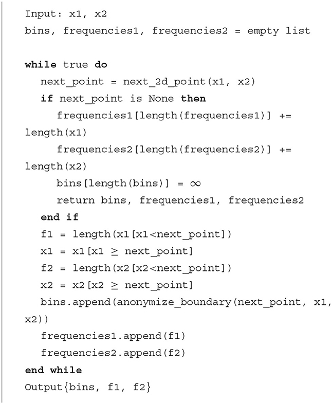
Algorithm 1. Binning algorithm.
The process proceeds (arbitrarily) from small to large values. The first bin is, initially, from a0 to a1, where a0 is the minimal value in the data and a1, is the smallest data value for which [ao, a1] has at least K observations from one group and either 0 or at least K observations from the other group. The next tentative bin limit, a2, is found in the same way, looking at the interval (a1, a2]. This continues so long as a new bin limit can be found. When a limit cannot be found, the number of unbinned data in at least one group is between 0 and K. Tentatively extend the upper limit of the previously formed bin to the maximal value of this group as the next limit. The unbinned data from the other group might permit continuation of the process, blocking off new bins in which that group has counts of at least K, vs. counts of 0 for the first group. When that group has fewer than K unbinned data, replace the last bin limit by the maximal value in the second group (See Algorithm S1 in Supplementary material for details.).
The initial bin boundaries a0, …, aB produced by the algorithm above are actual data values and, unless many subjects share the same value, violate the privacy condition. There is a simple fix for a1, …, aB−1. All values in the jth bin are ≤ aj and all values in the j+1st bin are >aj. So we can replace aj by cj = waj+(1−w)vj+1 where vj+1 is the smallest value in the (j+1)st bin and w is a uniform random variable on (0, 1). The extreme boundaries a0 and aB are the minimum and maximum in the data, so a different approach is needed. One option is to take c0 = −∞ and cB = ∞. Another option is to impose natural limits; for example, if by definition a variable cannot assume negative values, we could choose c0 = 0. A final option is to extend the bin limits by “privacy buffers”. To make these reasonably close to the data, we base them on the observed gaps between successive observations in the extreme bin. For example, compute cB as , where is the mean difference between consecutive data points in the last bin. (If , cB = aB, but this is now privacy preserving, as all observations in the last bin are equal to one another, with more than K in each group that has data.) Similarly, compute c0 as .
A new algorithm is needed to add the data from a new center, preserving all bin boundaries from the first center. The simple option of increasing the frequency counts in each current bin is not an option, as the incremental table from the new center will typically not be K-anonymous. Further, the incremental counts for some existing bin might be so large that data from the new center could actually be used to split it into two or more bins.
Algorithm S3 in Supplementary material is used to add the information from a new center to an existing summary table. We first iterate over the current bins, creating finer bins if possible. Then we remove any counts that are not K-anonymous by combining and redistributing data from adjacent cells. Pseudo-code for Algorithm S3 and for two algorithms called by it are given in the Supplementary material.
Splitting an existing bin into two bins forces us to reallocate the previous frequencies. We do so proportionally to the relative frequencies from the new center. For example, suppose a bin with a current count of 27 for one group is split into two new bins, which have equal counts at the new center. Then we split the 27 equally to the two new groups, adding 13.5 to each. Note that this procedure can result in counts that are not integers.
After creating new bins wherever possible, we iterate again and fix bins where the new center has frequencies between 0 and K. Proceeding from bin 1 to bin B, these non-private bins are combined with the next bin to the right until all counts from the new center are either 0 or at least K. Then the total counts are distributed among the original bins proportionally to the relative frequencies of the bins in the current table. Supplementary Table 1 shows an example that illustrates how the algorithm works.
The extreme bin limits c0 and cB must be compared with the minimum and maximum values, respectively, in the new center. If the new center has a more extreme data value, we need to revise these bin limits. We do so by applying the buffer method that was used to find c0 and cB in the largest center, but now adding buffers that depend only on the data in the extreme bin from the new center.
This section considers the problem of hypothesis testing with federated data, studying the common problem of determining whether numerical outcomes from two groups come from the same distribution (the null hypothesis, H0); or whether one group has larger values than the other. The standard choice is the independent samples t-test, which requires the mean, the standard deviation and the number of observations in each group. All of these are privacy-preserving summary statistics, so the t-test can still be used with federated data. However, the t-test relies on the assumption, often invalid, that the data are normally distributed. We consider here the standard non-parametric alternative, the Mann-Whitney U (“MWU”) test [9] (or, equivalently, the Wilcoxon rank sum test).
The MWU statistic can be defined as follows. Denoting the observations in the two groups by X1, …, Xn and Y1, …, Ym,
with
If H0 is true, the expected value of U is 0 and its variance is , where N = n+m, D is the number of distinct values in the data, and tr is the number of observations that share the rth distinct value. The second term corrects the variance for the presence of ties in the data. If c∈ℝ, the distribution of U is stochastically increasing as a function of c. The power of the test depends on P(Y>X) and is high when this probability differs from 0.5.
The MWU test involves direct comparison of each data point in one group with each data point from the other group. As this includes comparisons of observations from different centers, it is impossible to compute the MWU statistic for a federated analysis. Two broad options are possible for federated analysis.
• Compute the MWU statistic separately for each center and then combine them across centers.
• Generate a federated table summarizing the data from all the centers and then compute the MWU statistic on the federated table.
The next subsections present options for combining center-specific MWU statistics and the second analysis option, used in conjunction with our federated binning algorithm.
Denote by Ul the MWU from the lth center, based on nl and ml observations from the two groups, with Nl = nl+ml; and denote by Vl its variance under H0. A simple way to form a federated test statistic is to sum the individual statistics over the centers and normalize them by their standard deviation, leading to
A simple generalization is to replace the sum of the statistics by a weighted sum, with an optimal choice of weights. It is convenient to do this using the normalized test statistics for each center, . The weighted test statistic is then
The choice of weights can be made to maximize the power of the test when the null hypothesis is not true, using the fact that
where δl is the standardized effect in center l. For the MWU statistic, the standardized effect can be expressed as
where and in center l. Although the formula permits the probability difference to vary over centers, the natural basis for defining the weighted sum statistic is to assume a constant difference, in which case the optimal weights depend on the sample sizes and, if present, the extent of tied data. See Equation S1 in the Supplementary material for derivation of the weights.
Fisher's method [23] combines the p-values from independent samples. The corresponding statistic is where pl is the p-value from the MWU test result in the lth center.
We can compute the MWU statistic from the federated summary table generated by the algorithm described in Section 3. The table will have B bins whose frequencies are fxi and fyi. The frequencies sum to the total amount of data over all the centers, but need not be integers.
The MWU statistic for the federated table compares observations on the basis of their bins and is given by
where c0<c1 < ⋯ < cB are the endpoints of the bins and
The variance of Ufed can be computed from the formula in Section 4.1, keeping in mind that all observations in the same bin are tied.
A simulation study was used to compare the different federated MWU tests to an analysis of the combined data. Our goals are to assess how the federated analysis affects the power of the tests, and to use the power analysis to compare the testing methods. We also vary the simulation settings to examine how the results and comparisons are affected by the number of centers in the study and by heterogeneity across centers.
We simulated situations with 1,500 observations in each group, divided over 3, 5, or 10 centers, with the number of observations unbalanced among the centers (see Table 1).
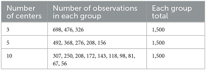
Table 1. Observations per center.
For the Mann-Whitney test, only the order of the observations is important, so any distribution can be used to simulate the data. Our model generates control group observations at center l as
and treatment group observations as
The possibility that centers may differ from one another is represented by . The difference between treatment and control at center l is where δ is the overall difference, and σβ represents heterogeneity of the treatment effect across centers. The terms ϵil, ϵjl~N(0, 1) are random errors. All random variables are independent of one another.
We simulated experiments with several different combinations of input parameters. We chose σα∈{0, 0.1, 0.2} and σβ∈{0, 0.05, 0.06} to achieve between center variance, and δ∈{0, 0.05, 0.1}. Including δ = 0 allowed us to verify that the tests remain reliable when both groups have the same mean. Note, however, that the variance is slightly larger for the treatment group if σβ>0, so that this setting does not fully match the null hypothesis of identical distributions.
Supplementary Figure 1 shows the distributions of p-values for all the tests in the null setting δ = 0. The left panel includes heterogeneity across centers (σα = 0.1), but no effect heterogeneity, and shows a uniform distribution for all the tests, as desired. The right panel adds a small amount of effect heterogeneity (σβ = 0.05. This results in a slightly wider spread of p-values for all the tests, so that actual type 1 errors are inflated from their nominal values. The fraction of p-values below 0.05 (0.01) was approximately 0.08 (0.025). The inflation was slightly weaker when more centers were included and slightly larger only for Fisher's test. The additional bias of Fisher's test is not surprising, as it is sensitive to the existence of an effect within a center, but not to having a consistent direction of the effect.
Figure 1 compares methods when δ≠0 across different parameters and numbers of centers. See also Supplementary Table S1. The federated table and weighted tests have p-value distributions that are very similar to those from combining all the data, indicating almost no loss of power. The sum test has higher p-values, hence consistently lower power. The p-values with Fisher's method are a bit higher when the treatment effect is consistent across centers (σβ = 0). When the effect is not consistent, they are lower. However, as already seen, Fisher's test in this case fails to preserve type 1 error, with a bias toward low values.
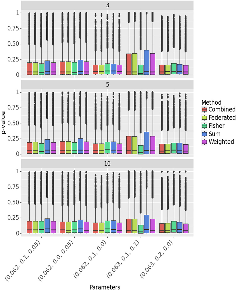
Figure 1. Comparison of methods across different parameters and number of centers. Panels represent the number of centers, the Y-axis presents the p-values and the X-axis the parameters (δ, σα, σβ). The different methods are color-coded.
Figure 2 focuses on how closely the federated test results compare with those from the combined test (i.e., using the full data) by comparing the p-values of each method on the same simulated data set. The Y axis presents log(piv/pis) where i represents the simulation number, s is the combined test and v is the federated test. A federated test that produces the same p-values as the combined test has no loss of power. The more tightly concentrated are these distributions around 0, the more nearly identical are the p-values of the federated method to those of the combined method.
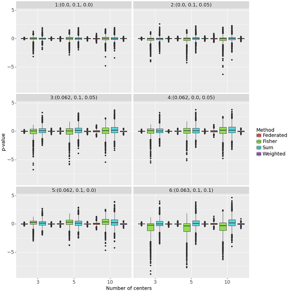
Figure 2. The figure shows log(piv/pis) on the Y axis, where s is the combined data analysis. The panels correspond to the different parameter settings for (δ, σα, σβ). The number of centers is on the X axis and the methods are color-coded.
Across all the settings, the weighted test most closely replicates the p-value of the combined test. The federated table is also similar, but more variable, especially when δ≠0. In the top left panel, where H0 is true, all methods are similar to the combined test. However, adding treatment heterogeneity (top right panel) induces bias in the p-values from Fisher's test, which will reject the null hypothesis too often. It also increases the variance of the log ratio for that test and for the sum. In all the settings with center heterogeneity (σα>0), the sum test gave, typically, slightly higher p-values than the combined test, hence had lower power.
To assess the power of the tests as a function of the effect size, we simulated p-values over a set of 4 increasing values of δ, when σα = 0.1 and σβ = 0.05. Figure 3 compares the methods to the unconstrained test using log(piv/pis) (Y-axis) where i represents the simulation number, s is the unconstrained method and v is the other method. Again the weighted test is most similar to the combined test, followed by the federated table. Table 2 shows the median of the p-value distributions with 10 centers; smaller medians correspond to higher power for the test. The medians for the weighted test are consistently the lowest ones; with even the modest heterogeneity present here, they are lower even than those for the combined test. The test from our federated table has slightly higher medians throughout than does the combined test. Similar quantiles were found for 3 and for 5 centers, indicating that, for the settings we examined, the number of centers has little effect on power.
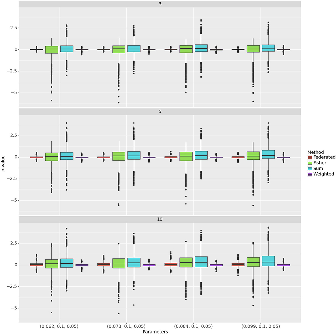
Figure 3. Comparison of methods across different parameters and number of centers. Rows correspond to the number of centers and segments within rows represent hyper-parameter configurations. The Y-axis represents the p-values. The methods are color-coded.
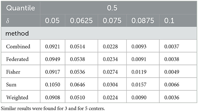
Table 2. Comparison of the tests for different values of δ with 10 centers when σα =.1, σβ =.05, and the 0.5 quantile of the p-value distributions.
This section considers the problem of quantile estimation when data are located in different centers. Quantile estimates are valuable for directing visual summaries of data distributions such as histograms or Kaplan-Meier plots. Standard methods for computing sample quantiles cannot be used, as they begin by ordering all the data, violating privacy. We propose and compare several methods for federated quantile estimation. Throughout we denote by F(x) the CDF and by the pth quantile of the distribution.
A quantile can be estimated as the solution to a minimization problem,
where the target function is the quantile loss function. The optimization can be carried out on federated data by returning function and gradient values from each center, proceeding iteratively to compute . The need for an iterative algorithm to minimize the loss, has the drawback of communication inefficiency.
A more serious concern is that the quantile loss compromises privacy. The loss function within each center is piecewise linear with a change in derivative at each data value in the center. Thus the information from a collection of calls can be used to recover the original data values at the federated node.
Despite the privacy violation, we will include in the subsequent comparisons as a benchmark.
It is possible to exploit the loss function to compute approximate quantile estimators that are differentially private [24].
The binning algorithm we introduced in Section 3 can be used to compute a federated estimate of Qp that is K-anonymous. Here, we apply the single group version of the algorithm which gives a summary table that has B bins with endpoints b0<b1<b2 < ⋯ < bB and frequencies fx, k. Let denote the cumulative distribution for the federated table at bi.
A naive estimate is the smallest bin limit with cumulative frequency greater than 100p% of the data. However, restricting Qp to the set of bin limits is an obvious drawback, especially for quantiles in the tails of the distribution. A simple improvement is to interpolate the estimated CDF from one bin limit to the next. Linear interpolation corresponds to the assumption of a uniform distribution within each bin. That may be reasonable for bins in the center of the data. However, it is not likely to work well in the tails, especially in the most extreme bins. We did attempt to use linear interpolation, but the results were poor and are not reported here.
We propose here a more sophisticated interpolation method based on the Yeo-Johnson transformation (“YJ”) [25], a power transformation used to achieve a distribution that is closer to the normal. The approach extends the well-known Box-Cox [26] transformation to also handle variables that can take on negative values. The transformation is defined by
In this method, the goal is to find values of λ, a0 and a1 for which the transformed bin limits approximately match a normal distribution with mean a0 and standard deviation a1,
where bk is a bin limit, is the estimator of the distribution function from the federated table and hλ(x) is the (“YJ”) [25] transformation. The quantile Qp is then estimated by
Given λ, we can compute a0, a1 using linear regression. To estimate λ, we use the idea that an effective transformation hλ should have transformed quantiles that are linearly related to the YJ-estimated quantiles. This can be achieved by choosing λ to maximize the correlation between them,
where the values of X we use are the interior bin limits b1, …, bB−1.
Note that the range of the inverse transformation in 5 is given by
To ensure that the inverse transformation has values in ℝ we set the constraint 0 ≤ λ ≤ 2 for equation 8.
The YJ Table method is a “one pass” algorithm, calling the data only to produce the federated summary table. Thus it enjoys full communication efficiency.
The parameters in the YJ transformation can also be estimated by maximum likelihood. Denoting by xil the observations from center l and by N the total number of observations, the log likelihood is
where
For a fixed value of λ, the log-likelihood requires only summary statistics from each center, so can be computed in a federated manner. This can be embedded in a simple optimization routine that maximizes the log likelihood over λ.
As with the quantile loss, the YJ likelihood method employs an iterative algorithm, and thus is not communication efficient. However, unlike the quantile loss, the YJ log likelihood for each center is not a simple function of the data that can be immediately inverted to recover data values. Thus the privacy violations of the quantile loss do not occur here.
Once we have , we can again use summary statistics from the centers to compute . The resulting quantile estimator is
The likelihood maximization is iterative, so requires multiple communication steps with each center. By contrast, the methods based on the federated table are “one pass”, requiring just one call to each center. This communication inefficiency of the maximum likelihood method can be improved by submitting to each center a grid of possible λ values. The centers then return the moments needed to compute the log likelihood for each value in the grid. The resulting estimate of λ can either be the best value among those in the grid or the maximizer of an empirical fit to the relationship between the log likelihood and λ. The result is an approximate, one pass MLE.
Federated quantile estimates can be used to generate an alternative summary table, which presents a collection of quantiles. See Table 3 for an example, with estimates from optimizing the quantile loss and the YJ likelihood.
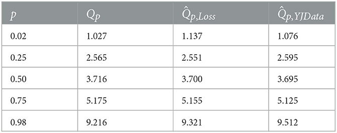
Table 3. A summary table constructed from quantile estimates, based on 1,500 observations from 3 centers, with a mixed gamma distribution.
We compared the three quantile estimators using a simulation configuration similar to that in the testing chapter. As the quantiles are univariate summaries, we generated data and estimated quantiles only in one group. Another important difference is that the form of the underlying distribution affects the estimation results. In particular, methods may vary when faced with long rather than short tails. To gain insight into this issue, we chose the Gamma as the base distribution for assessing the quality of quantile estimation.
Each simulated data set included 1,500 observations, spread across 3, 5, or 10 centers exactly as described in Table 1. The observations were generated from the following model: xil = ϵilexp(αl) where xil is observation i at center l with and ϵil~Gamma(r, 1) r∈{4, 10}. The skewness of Gamma is , so the smaller value for r has a longer right tail.
For the Gamma data, heterogeneity across centers was induced using scale rather than location shifts. The value of σα was chosen to achieve between center heterogeneity similar in extent to that in Section 4. There the key term was the ratio σα/σϵ, which was taken to be 0, 0.1 or 0.2. With Gamma data, the standard deviation of the homogeneous data is proportional to the median, so the analogous choice is to set , with ϕ similar to the values chosen above. We used only ϕ = 0.1 in our simulations for quantile estimation.
For each combination of the parameters, 2,000 simulations were run. The true quantile Qp for each simulation was computed from the mixture (over centers) distribution by solving the equation below with l as the center index.
where N is the number of observations from all centers, nl the observations in center l and Γr is the standard Gamma CDF with shape parameter r. A dominant part of the quantile estimation errors is the natural variability of the underlying Gamma distribution. As the standard deviation for Gamma(r, 1) is , we summarized results via the normalized estimation error where is the estimator of Qp.
The simulation results for estimating Q0.98 are shown in Figure 4. This quantile is presented separately, as it is the most challenging case, in the right tail of a right-skewed distribution. Results for Q0.02,Q0.25,Q0.5, Q0.75 are depicted in Figure 5. Further detail is provided in Supplementary Tables S2–S5, which give, respectively, the estimated bias and standard deviation, the mean squared error (MSE), and the ratio of squared bias to variance for all the methods and all the quantiles.
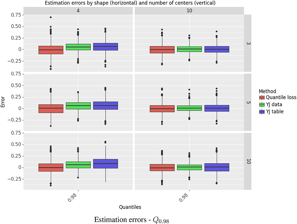
Figure 4. Estimation errors - Q0.98. The figure shows the standardized errors, (on the Y axis) for estimating the 98th quantile. Each column represents the shape r and each row the number of centers. The methods are color-coded. The rest of the quantiles are depicted separately in Figure 5 due to having a different error scale.
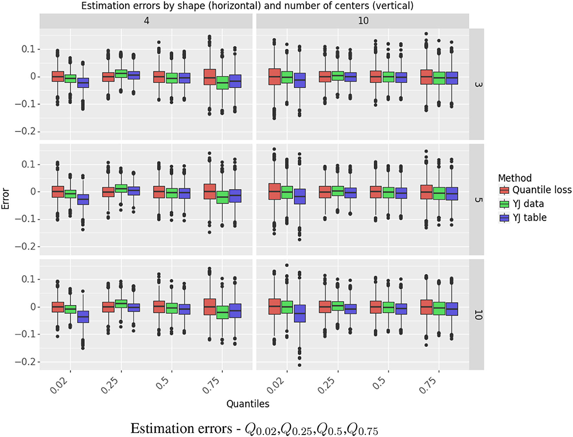
Figure 5. Estimation errors - Q0.02,Q0.25,Q0.5,Q0.75. The figure shows the standardized errors, (on the Y axis) for estimating the quantiles (on the X axis). Each column represents the shape r and each row the number of centers. The methods are color-coded.
The YJ data estimator achieved lower MSE than the quantile loss estimator. For the extreme quantiles, the decrease in MSE ranged from 14% to 44%. The “one pass” YJ table estimator was very accurate for estimating the median and the quartiles, but lost efficiency for the extreme quantiles with the more skewed of the two Gamma distributions and when the number of centers was large. In that setting, the estimator for Q0.02 suffered from negative bias and its MSE was almost 3 times as large as for the quantile loss estimator; the MSE for Q0.98 was about 80% larger.
For the settings we studied, variance was the dominant component of MSE. Bias was a substantial problem only in a small number of cases. The YJ methods had large positive bias for Q0.98 when r = 4; however, when r = 10, and the distribution is itself closer to normal, the bias was negligible.
In this work we presented novel methods for federated data analysis and investigated their statistical properties. We proposed a simple algorithm for creating K-anonymous data tables in one- and two-group problems and we compared federated approaches for the non-parametric Mann-Whitney U (MWU) test and for estimating quantiles. Our federated data table is created in a “one pass” format, so that it is communication efficient.
For the MWU test, we found that the most powerful method was the weighted average of the MWU statistics from the individual centers, with weights reflecting the sample sizes. This statistic is also communication efficient, gives nearly identical p-values to those from the combined data and has the advantage of adjusting for inter-center heterogeneity, effectively treating each center as a block. The logged ratios of p-values from this method to those from the MWU test on the combined data were heavily concentrated around 0. With increasing effect sizes, the median p-value from the weighted MWU test was lower than that for the combined test, so actually increases power. The test based on our federated table was slightly less effective. The logged ratios of p-values were still strongly concentrated around 0, but with more spread than for the weighted average. With increasing sample size, the median p-values were slightly larger than those for the combined test. Thus, both of these tests will have almost identical power to the combined data test regardless of the level of significance desired.
For quantile estimation, the fully optimized YJ method consistently had the lowest MSE of the methods we compared. For the extreme quantiles, it improved by 14% to 44% over the quantile loss estimator. The “one pass” YJ table estimator had almost identical MSE for estimating the median and the quartiles, but lost efficiency for the extreme quantiles when the number of centers was large. The increase in MSE was more substantial (almost 80%) with the more skewed of the two Gamma distributions we studied. This is not surprising: our YJ method exploits a transformation to normality and is less successful when the distribution is further from the normal.
It is important that research on federated data analysis will relate to statistical efficiency and not just to algorithmic efficiency. Our work opens this avenue, but much more could be done. Here are some examples. One important extension is to consider the impact of federated analysis on a wider range of statistical inference procedures. Another needed direction is to consider alternative mechanisms for privacy protection and to compare them with respect to the loss in statistical efficiency. Our proposals raise a number of specific questions. The construction method for a federated summary table could be extended to multiple variables and to higher dimensions; our method creates the bins in a way fitted to a one-dimensional variable. This would be needed, for example, to produce a federated analog of a scatter plot. Our findings suggest that heterogeneity can harm the federated analysis. Methods are needed to identify heterogeneity and to account for it in the analysis. The investigation of quantile estimators could be extended to a wider class of distributions. Our implementation of the YJ method applies a single transformation to the distribution. For quantiles in the tails of the distribution, it might be better to use separate transformations in the left and in the right tails.
Our results, like those of [21], are encouraging for the use of federated statistical analysis. We show that the Mann-Whitney U test and quantile estimation can be used at close to full efficiency on federated data with the K-anonymity constraint (for K = 10). Similarly, Spath et al. [21] found little loss of efficiency for time-to-event analyses when differential privacy is applied. We do point to some potential problems, for example in coping with inter-center heterogeneity. At the same time, the challenges of federated statistical analysis can also stimulate more efficient methods; our use of the Yeo-Johnson transformation improved upon the standard quantile estimator for most of the settings examined. In any particular setting, we advise researchers to carefully assess the choice of methods for their analyses. As we show, efficiency also depends on how many centers are being federated, how diverse are the data across centers, and what statistical methods will be used for the analysis. The simulation framework that we describe and exploit here can be applied to assess and compare options.
Publicly available datasets were analyzed in this study. This data can be found at: https://github.com/oribech/federated-summary-table.
DMS: Conceptualization, Funding acquisition, Methodology, Supervision, Writing—original draft, Writing—review & editing. OB: Conceptualization, Formal analysis, Investigation, Methodology, Software, Writing—original draft, Writing—review & editing. MM-K: Conceptualization, Funding acquisition, Methodology, Writing—review & editing.
The author(s) declare financial support was received for the research, authorship, and/or publication of this article. This research has received funding from the European Union's Horizon 2020 Framework Programme for Research and Innovation under the Specific Grant Agreement No. 785907 (Human Brain Project SGA2) and the Specific Grant Agreement No. 945539 (Human Brain Project SGA3).
The authors declare that the research was conducted in the absence of any commercial or financial relationships that could be construed as a potential conflict of interest.
All claims expressed in this article are solely those of the authors and do not necessarily represent those of their affiliated organizations, or those of the publisher, the editors and the reviewers. Any product that may be evaluated in this article, or claim that may be made by its manufacturer, is not guaranteed or endorsed by the publisher.
The Supplementary Material for this article can be found online at: https://www.frontiersin.org/articles/10.3389/fams.2023.1267034/full#supplementary-material
1. Proietti R, Rivera-Caravaca JM, Lopez-Galvez R, Harrison SL, Buckley BJR, Marin F, et al. Clinical implications of different types of dementia in patients with atrial fibrillation: insights from a global federated health network analysis. Clin Cardiol. (2023) 46:656–62. doi: 10.1002/clc.24006
2. Shiri I, Vafaei Sadr A, Akhavan A, Salimi Y, Sanaat A, Amini M, et al. Decentralized collaborative multi-institutional PET attenuation and scatter correction using federated deep learning. Eur J Nuclear Med Mol Imaging (2023) 50:1034–50. doi: 10.1007/s00259-022-06053-8
3. Annie FH, Embrey S, George H, Gwinn R, Mandapaka S, Mukherjee D, et al. Effect of sex differences in TAVR mortality using a federated database. J Am Coll Cardiol. (2021) 77(18_Suppl _1):3370. doi: 10.1016/S0735-1097(21)04724-0
4. Pati S, Baid U, Edwards B, Sheller M, Wang SH, Reina GA, et al. Federated learning enables big data for rare cancer boundary detection. Nat Commun. (2022) 13:7346. doi: 10.1038/s41467-022-33407-5
5. Ogier du Terrail J, Leopold A, Joly C, Beguier C, Andreux M, Maussion C, et al. Federated learning for predicting histological response to neoadjuvant chemotherapy in triple-negative breast cancer. Nat Med. (2023) 29:135–46. doi: 10.1038/s41591-022-02155-w
6. Salles A, Stahl B, Bjaalie J, Domingo-Ferrer J, Rose N, Rainey S, et al. Opinion Action Plan on ‘Data Protection Privacy' (Human Brain Project). (2017). Available online at: https://sos-ch-dk-2.exo.io/public-website-production/filer_public/24/0e/240e2eaa-8a10-4a17-87bc-b056a3f0cc8c/opinion_on_data_protection_and_privacy_done_01.pdf
7. Samarati P, Sweeney L. Protecting Privacy When Disclosing Information: k-Anonymity and Its Enforcement Through Generalization and Suppression. SRI International Computer Science Library (1998).
8. Dwork C. Differential privacy. In:Bugliesi M, Preneel B, Sassone V, Wegener I, , editors. Automata, Languages and Programming. Berlin; Heidelberg: Springer (2006). p. 1–12.
9. Mann HB, Whitney DR. On a test of whether one of two random variables is stochastically larger than the other. Ann Math Stat. (1947) 18:50–60. doi: 10.1214/aoms/1177730491
10. Yang Q, Liu Y, Chen T, Tong Y. Federated machine learning: concept and applications. arxiv preprint arxiv:1902.04885 (2019). doi: 10.48550/ARXIV.1902.04885
11. Li Q, Wen Z, Wu Z, Hu S, Wang N, Li Y, et al. A survey on federated learning systems: vision, hype and reality for data privacy and protection. IEEE Trans Knowledge Data Eng. (2021) 35:3347–66. doi: 10.1109/2Ftkde.2021.3124599
12. Kairouz P, McMahan HB, Avent B, Bellet A, Bennis M, Nitin Bhagoji A, et al. Advances and open problems in federated learning. Found Trends Mach Learn. (2021) 14:1–210. doi: 10.1561/2200000083
13. McMahan HB, Moore E, Ramage D, Hampson S, Bay A. Communication-efficient learning of deep networks from decentralized data. arxiv preprint arxiv:1602.05629 (2016). doi: 10.48550/ARXIV.1602.05629
14. Li T, Sahu AK, Talwalkar A, Smith V. Federated learning: challenges, methods, and future directions. IEEE Signal Process Magaz. (2020) 37:5060. doi: 10.1109/MSP.2020.2975749
15. Li X, Jiang M, Zhang X, Kamp M, Dou Q. Fed{bn}: federated learning on non-{iid} features via local batch normalization. In: International Conference on Learning Representations. (2021).
16. Hwang H, Yang S, Kim D, Dua R, Kim JY, Yang E, et al. Towards the practical utility of federated learning in the medical domain. In:Mortazavi BJ, Sarker T, Beam A, Ho JC, , editors. Proceedings of the Conference on Health, Inference, and Learning. New York, NY: PMLR (2023). p. 163–81.
17. Nasirigerdeh R, Torkzadehmahani R, Matschinske J, Frisch T, List M, Späth J, et al. sPLINK: a federated, privacy-preserving tool as a robust alternative to meta-analysis in genome-wide association studies. bioRxiv. (2020). doi: 10.1101/2020.06.05.136382
18. Duan R, Boland MR, Liu Z, Liu Y, Chang HH, Xu H, et al. Learning from electronic health records across multiple sites: A communication-efficient and privacy-preserving distributed algorithm. J Am Med Inform Assoc. (2019) 27:376–85. doi: 10.1093/jamia/ocz199
19. Duan R, Boland MR, Moore JH, Chen Y. ODAL: A one-shot distributed algorithm to perform logistic regressions on electronic health records data from multiple clinical sites. In: Pacific Symposium on Biocomputing (2019). p. 30–41.
20. Liu Q, Ihler A. Distributed estimation, information loss and exponential families. In:Ghahramani Z, Welling M, Cortes C, Lawrence N, Weinberger KQ, , editors. Advances in Neural Information Processing Systems. Curran Associates, Inc. (2014). Available online at: https://proceedings.neurips.cc/paper_files/paper/2014/file/303ed4c69846ab36c2904d3ba8573050-Paper.pdf
21. Spath J, Matschinske J, Kamanu FK, Murphy SA, Zolotareva O, Bakhtiari M, et al. Privacy-aware multi-institutional time-to-event studies. PLoS Digit Health. (2022) 1:e0000101. doi: 10.1371/journal.pdig.0000101
22. Rosenblatt JD, Nadler B. On the optimality of averaging in distributed statistical learning. Inform Inference. (2016) 53:79–404. doi: 10.1093/imaiai/iaw013
24. Kaplan H, Schnapp S, Stemmer U. Differentially private approximate quantiles. In: Proceedings of the 39th International Conference on Machine Learning. (2022). p. 10751–61.
25. Yeo IK, Johnson RA. A new family of power transformations to improve normality or symmetry. Biometrika. (2000) 87:954–9. doi: 10.1093/biomet/87.4.954
Keywords: federated analysis, Mann-Whitney test, medical informatics, privacy preservation, information loss
Citation: Becher O, Marcus-Kalish M and Steinberg DM (2023) Federated statistical analysis: non-parametric testing and quantile estimation. Front. Appl. Math. Stat. 9:1267034. doi: 10.3389/fams.2023.1267034
Received: 25 July 2023; Accepted: 03 October 2023;
Published: 13 November 2023.
Edited by:
Jun Fan, Hong Kong Baptist University, Hong Kong SAR, ChinaReviewed by:
Giovanni Cicceri, University of Messina, ItalyCopyright © 2023 Becher, Marcus-Kalish and Steinberg. This is an open-access article distributed under the terms of the Creative Commons Attribution License (CC BY). The use, distribution or reproduction in other forums is permitted, provided the original author(s) and the copyright owner(s) are credited and that the original publication in this journal is cited, in accordance with accepted academic practice. No use, distribution or reproduction is permitted which does not comply with these terms.
*Correspondence: David M. Steinberg, ZG1zQHRhdWV4LnRhdS5hYy5pbA==
Disclaimer: All claims expressed in this article are solely those of the authors and do not necessarily represent those of their affiliated organizations, or those of the publisher, the editors and the reviewers. Any product that may be evaluated in this article or claim that may be made by its manufacturer is not guaranteed or endorsed by the publisher.
Research integrity at Frontiers
Learn more about the work of our research integrity team to safeguard the quality of each article we publish.