Some finite difference methods for solving linear fractional KdV equation

The time-fractional Korteweg de Vries equation can be viewed as a generalization of the classical KdV equation. The KdV equations can be applied in modeling tsunami propagation, coastal wave dynamics, and oceanic wave interactions. In this study, we construct two standard finite difference methods using finite difference methods with conformable and Caputo approximations to solve a time-fractional Korteweg-de Vries (KdV) equation. These two methods are named as FDMCA and FDMCO. FDMCA utilizes Caputo's derivative and a finite-forward difference approach for discretization, while FDMCO employs conformable discretization. To study the stability, we use the Von Neumann Stability Analysis for some fractional parameter values. We perform error analysis using L₁ & L_∞ norms and relative errors, and we present results through graphical representations and tables. Our obtained results demonstrate strong agreement between numerical and exact solutions when the fractional operator is close to 1.0 for both methods. Generally, this study enhances our comprehension of the capabilities and constraints of FDMCO and FDMCA when used to solve such types of partial differential equations laying some ground for further research.

1 Introduction

Fractional partial differential equations (FPDEs) are a generalization of classical partial differential equations (PDEs) that involve fractional derivatives of arbitrary order. The fractional derivatives in FPDEs account for non-local and non-linear phenomena, which are not captured by classical PDEs [1]. Physical models of real-world phenomenon often comprise considerable uncertainty due to a variety of variables. Due to their ability to model complex phenomena in physics and engineering, FPDEs have gained significant attention in recent years with their applications in signal processing, mechanics, plasma physics, finance, electricity, stochastic dynamical system, control theory, economics, and electrochemistry [2–4]. The numerical solution of fractional partial differential equations (FPDEs) has some challenges due to the non-local and non-linear nature of the fractional derivatives [5]. The Korteweg-de Vries (KdV) equation is a mathematical equation utilized to explain various physical phenomena related to non-linear wave evolution and interaction. It was developed based on the propagation of shallow water waves and is widely applied in areas such as fluid dynamics, aerodynamics, and continuum mechanics to model solitons, turbulence, and boundary layers, among others [6].

Several techniques have been developed to construct analytical and numerical methods for the KdV equation. These include the Adomian decomposition method [7], homotopy perturbation method [8], variational iteration method [9], finite difference method [10], and finite volume method [11]. Aderogba and Appadu [12] recently used classical and multisymplectic schemes to solve some linearized KdV equations and dispersion analysis was studied. The authors in Appadu and Kelil [10] conducted a comparative study involving the application of the modified Adomain Decomposition Method and the classical finite difference method for solving some third-order and fifth-order KdV equations. Rostamy et al. [13] presented a numerical method for solving a class of fractional differential equations based on Bernstein polynomials basis; these matrices are utilized to reduce the multi-term orders fractional differential equation to a system of algebraic equations. Anwar et al. [14] studied the double Laplace formulae for the partial fractional integrals and derivatives in the sense of Caputo.

In studies, there are many formulations for the fractional differentiation and integration operators, including the Riemann-Liouville definition [15] and the Caputo definition [4]. A quite recent definition of the fractional derivative called the conformable fractional derivative, which can address the drawbacks of several definitions, was proposed by Khalil et al. [16]. The conformable operators generalize the classical idea of differentiability and allow for the generation of new and universal rates of variation. Therefore, the novelty of the study by Khalil et al. [16] was to check the validity of these operators together with classical finite difference approach in creating a new environment to look for more extended natural dispersive modeling scenarios. Toprakseven [17] derived a reliable finite difference method for fractional differential equations (FDEs) based on recently defined conformable fractional derivative. Li and Xu [18] constructed a time-space spectral method to investigate the solution of fractional partial differential equation. Lin and Xu [19] obtained the error estimate of the L1 scheme.

The plan of this study is detailed below. Section 2 describes the numerical experiment. In Section 3, we give some background on conformable fractional order derivative for the solution of non-homogeneous KdV equations. In Section 4, we propose a finite difference scheme known as the FDMCO scheme, which utlilizes the conformable derivative. We have conducted a comprehensive study on stability analysis and consistency of the FDMCO scheme. Section 5 provides numerical results obtained from the FDMCO scheme, offering valuable insights into its performance, under various fractional parameter values α∈(0, 1]. Section 6 proposes a finite difference scheme using Caputo fractional derivative and results shown in Section 7, respectively. Numerical profiles and relative errors for FDMCA scheme is given in subsection 7.2. Discussion of the comparison between the two schemes and conclusions are given in Section 8.

2 Numerical experiment

The Korteweg-de Vries (KdV) equation, introduced in 1895, describes weakly non-linear, dispersive waves, featuring non-linear advection and dispersion. The fractional Korteweg-de Vries (KdV) equation, as a generalization of the classical KdV equation, motivated by complex phenomena in dispersive media and takes the form:

$\frac{{\text{∂}}^{\alpha }u(t,x)}{\text{∂}{t}^{\alpha }}+u\frac{\text{∂}u(t,x)}{\text{∂}x}+\frac{{\text{∂}}^{3}u(t,x)}{\text{∂}{x}^3}=0.$

It uses fractional derivatives to analyze non-local effects and memory in wave propagation [4], providing insights into diverse problems by capturing intricate dynamics. These dynamics extend from fluid dynamics to plasma physics, encompassing long-range interactions, anomalous diffusion, and power-law behavior.

We consider the linear time-fractional non-homogeneous KdV equation [20] given by

$\begin{array}{ll}\frac{{\text{∂}}^{\alpha }u(t,x)}{\text{∂}{t}^{\alpha }}+\frac{\text{∂}u(t,x)}{\text{∂}x}+\frac{{\text{∂}}^{3}u(t,x)}{\text{∂}{x}^3}=2tcos(x),& (1)\end{array}$

where (t, x)∈[0, 1.0] × [0, 3π], and 0 < α ≤ 1. The initial condition is

$\begin{array}{ll}u(x,0)=0,& (2)\end{array}$

and the following boundary conditions are used:

$\begin{array}{ll}u(0,t)=\frac{2t^{\alpha +1}}{\mathrm{\Gamma }(2\alpha +1)};u(3\pi ,t)=-\frac{2t^{\alpha +1}}{\mathrm{\Gamma }(2\alpha +1)}.& (3)\end{array}$

The exact solution for this numerical experiment is given by Mohyud-Din et al. [20]

$\begin{array}{l}u(x,t)=2cos(x)\frac{t^{\alpha +1}}{\mathrm{\Gamma }(2\alpha +1)}.\end{array}$

We note that for α = 1, the exact solution is u(x, t) = t²cos(x). In this study, we have used spatial step size $\mathrm{\Delta }x=\frac{\pi }{10}$.

The relative error is calculated at a given spatial node x_j and time t_n using the following formula:

$\begin{array}{ll}\begin{array}{l}\text{Relative error}=\left|\frac{u(x_j,t_n)-U(x_j,t_n)}{u(x_j,t_n)}\right|\hfill \end{array},& (4)\end{array}$

subject to the condition that the exact solution u at the nodal point (x_j, t_n) is non-zero; U(x_j, t_n) represents the numerical solution at spatial domain x_j and time t_n. In this study, a scheme is considered efficient when its relative error is below 10%, and it is deemed satisfactory when the relative error falls within the range of 10% up to 25%. The scheme is considered to perform poorly if the relative error is greater than 25%. By relying on the given exact solution, the accuracy of the numerical solution and the performance (efficiency) of the scheme by computing L₁ and L_∞ errors using the formulations:

$\begin{array}{l}{L}_1={\parallel U^{\text{exact}}-U_N\parallel }_1=h{\displaystyle \sum _{j=0}^N}\left|U_j^{\text{exact}}-{(U_N)}_j\right|;\text{and}\\ L_{\infty }={\parallel U^{\text{exact}}-U_N\parallel }_{\infty }={\displaystyle \underset{j}{max}}|U_j^{\text{exact}}-{(U_N)}_j\parallel ,\end{array}$

respectively.

3 Fractional derivatives

There are few definitions of fractional derivatives of order α>0. The most widely used are the Riemann-Liouville (RL), Caputo and conformable fractional derivatives [1, 16, 21–23].

Definition 1. The Riemann-Liouville fractional integral is defined by

$\begin{array}{l}{J}_t^{\alpha }f(t)=\frac{1}{\mathrm{\Gamma }(\alpha )}{\displaystyle {\int }_0^t{(t-\tau )}^{\alpha -1}f(\tau )d\tau ,\alpha >0,}\hfill \end{array}$

where

$\mathrm{\Gamma }(\alpha )={\displaystyle {\int }_0^{+\infty }{x}^{\alpha -1}{e}^{-x}dx,}$

is the Euler Gamma function [4].

Definition 2. The Caputo time-fractional derivative operator of order α>0 (m−1 < α ≤ m, m∈ℕ) of a real valued function u(x, t) is defined as follows [24]:

$\begin{array}{l}\frac{{\partial }^{\alpha }u(x,t)}{\partial t^{\alpha }}=J_t^{m-\alpha }\left[\frac{{\partial }^{m}u(x,t)}{\partial t^m}\right],\\ =\{\begin{array}{l}\frac{1}{\mathrm{\Gamma }(m-\alpha )}{\displaystyle {\int }_0^t{(t-y)}^{m-\alpha -1}}\frac{{\partial }^{m}u(x,y)}{\partial y^m}\text{d}y,m-1<\alpha \le m,\\ \frac{{\partial }^{m}u(x,t)}{\partial t^m},\alpha =m.\end{array}& (5)\end{array}$

Similarly, the Caputo space-fractional derivative operator $\frac{{\partial }^{\alpha }u(x,t)}{\partial x^{\alpha }}$ of order α > 0 (m−1 < α ≤ m), m∈ℕ can be defined [22, 25]. It is worth noting that if u is sufficiently smooth [26], the fractional derivative ${\mathcal{D}}_t^{\alpha }u$ recovers the typical first-order derivative u′(t) as α → 1⁻ [25].

Definition 3. [16]. For a function g:[0, ∞] → ℝ, the conformable fractional derivative of g of order α is defined by

$\begin{array}{ll}{D}^{\alpha }\left\{g(z)\right\}={\displaystyle \underset{\eta \to 0}{lim}}\left(\frac{g(z+\eta z^{1-\alpha })-g(z)}{\eta }\right).& (6)\end{array}$

Fundamental concepts and properties of conformable calculus are given in Khalil et al. [16] and Abdeljawad [21], and we note that the conformable derivative is chosen in order to preserve some of the classical properties of classical calculus [21]. Since other popular fractional derivatives (Caputo, RL) lack some of the natural properties of derivatives such as product rule, quotient rule, and chain rule, some authors such as Khalil et al. [16], and Abdelwajad [21] motivate the need to study conformable derivative to fill these gaps of preserving some natural properties of derivatives [4, 25].

Abdelwajad [21] approximated the time-fractional derivative using conformable approximation

$\begin{array}{ll}\frac{{\partial }^{\alpha }u(x,t)}{\partial t^{\alpha }}={(\mathrm{\Delta }t)}^{1-\alpha }\frac{\partial u}{\partial t}.& (7)\end{array}$

if we let h = ηt^1−α, we thus have

$\begin{array}{l}\frac{{\partial }^{\alpha }g(t)}{\partial t^{\alpha }}=\underset{\eta \to 0}{\lim }\left(\frac{g(t+\eta t^{1-\alpha })-g(t)}{\eta }\right)\\ =t^{1-\alpha }\underset{h\to 0}{\lim }\left(\frac{g(t+h)-g(t)}{h}\right)\\ =t^{1-\alpha }\frac{\partial g(t)}{\partial t}.& (8)\end{array}$

Hence, we can approximate $\frac{{\partial }^{\alpha }u(x,t)}{\partial t^{\alpha }}$ by ${(\mathrm{\Delta }t)}^{1-\alpha }\left[\frac{U_j^{n+1}-U_j^{n-1}}{2·(\mathrm{\Delta }t)}\right],$ if we choose to use a central difference approximation for $\frac{\partial u}{\partial t}$.

For some properties of conformable fractional derivatives, we refer the reader to Khalil et al. [16], Abdelwajad [21], Atangana et al. [28], and Atangana and Secer [29].

Yokus et al. [27] conducted a comparative study on the time fractional Burgers-Fisher equation, specifically focusing on the Caputo and conformable approximations; and the authors utilized the sub-equation method as an analytical approach for their investigation. Yokus et al. [30] examined various methods, including analytical, numerical, and approximate analytical techniques, to solve the time-fractional non-linear Burger-Fisher equation. Specifically, they employed the (1/G')-expansion method, the finite difference method (FDM), and the Laplace perturbation method (LPM). Pedram et al. [31] studied the effect of white noise on conformable time and space fractional KdV and BBM equations by transforming these equations with external noise into homogeneous conformable time and space fractional KdV and BBM equations and solved these equations using the modified Kudryashov method. In Arafa et al. [32], the authors employed a time-fractional conformable derivative to investigate an unsteady convection-radiation interaction flow of power-law non-Newtonian nanofluids. Mous et al. [33] investigated the numerical solution of a coupled system of two-dimensional (2D) Burgers' equations with fractional conformable time derivatives,and they tried to capture the interaction between non-linear convection processes and diffusive viscous processes. Azerad and Bourharguane [34] constructed some finite difference schemes to solve a fractional diffusion/anti-diffusion equation, and they also studied the stability, consistency, and convergence of these schemes.

4 Finite difference method using conformable approximation

4.1 Derivation

We consider Equation (1) and discretise $\frac{\partial u}{\partial x}$ and $\frac{{\partial }^{3}u}{\partial x^3}$ using central difference approximations and approximate $\frac{{\partial }^{\alpha }u(x,t)}{\partial t^{\alpha }}$ using (??). This gives the following scheme which we term as “finite difference method using conformable derivative” abbreviated as FDMCO:

$\begin{array}{l}\begin{array}{l}{(\mathrm{\Delta }t)}^{1-\alpha }\left(\frac{U_j^{n+1}-U_j^{n-1}}{2(\mathrm{\Delta }t)}\right)+\left(\frac{U_{j+1}^n-U_{j-1}^n}{2(\mathrm{\Delta }x)}\right)\hfill \end{array}\\ \begin{array}{l}+\left(\frac{U_{j+2}^n-2U_{j+1}^n+2U_{j-1}^n-U_{j-2}^n}{2{(\mathrm{\Delta }x)}^3}\right)=2t_n\cos (x_j).\hfill \end{array}& (9)\end{array}$

Equation (9) is rewritten as

$\begin{array}{l}{U}_j^{n+1}=U_j^{n-1}-\frac{{(\mathrm{\Delta }t)}^{\alpha }}{\mathrm{\Delta }x}(U_{j+1}^n-U_{j-1}^n)\\ -\frac{{(\mathrm{\Delta }t)}^{\alpha }}{{(\mathrm{\Delta }x)}^3}(U_{j+2}^n-2U_{j+1}^n+2U_{j-1}^n-U_{j-2}^n).\\ +4(\mathrm{\Delta }t{)}^{\alpha }{t}_n\cos (x_j),& (10)\end{array}$

We need to use another scheme to obtain solution at second time level. The scheme is given by

$\begin{array}{l}\begin{array}{l}{(\mathrm{\Delta }t)}^{1-\alpha }\left(\frac{U_j^2-U_j^1}{\mathrm{\Delta }t}\right)+\left(\frac{U_{j+1}^1-U_{j-1}^1}{2(\mathrm{\Delta }x)}\right)\hfill \end{array}\\ \begin{array}{l}+\left(\frac{U_{j+2}^1-2U_{j+1}^1+2U_{j-1}^1-U_{j-2}^1}{2{(\mathrm{\Delta }x)}^3}\right)=2t_1\cos (x_j).\hfill \end{array}& (11)\end{array}$

which can be rewritten as

$\begin{array}{l}\begin{array}{l}{U}_j^2=U_j^1-\frac{{(\mathrm{\Delta }t)}^{\alpha }}{2(\mathrm{\Delta }x)}(U_{j+1}^1-U_{j-1}^1)\hfill \end{array}\\ -\frac{{(\mathrm{\Delta }t)}^{\alpha }}{2{(\mathrm{\Delta }x)}^3}(U_{j+2}^1-2U_{j+1}^1+2U_{j-1}^1-U_{j-2}^1),& (12)\end{array}$

where $U_j^1$ is the initial solution at the grid point x_j.

4.2 Stability analysis

To obtain the stability region of the scheme, we make use of Von Neumann Stability Analysis. We consider Equation (10) with source term being 0, i.e.,

$\begin{array}{l}{U}_j^{n+1}=U_j^{n-1}-\frac{{(\mathrm{\Delta }t)}^{\alpha }}{\mathrm{\Delta }x}(U_{j+1}^n-U_{j-1}^n)\\ -\frac{{(\mathrm{\Delta }t)}^{\alpha }}{{(\mathrm{\Delta }x)}^3}(U_{j+2}^n-2U_{j+1}^n+2U_{j-1}^n-U_{j-2}^n).& (13)\end{array}$

We use the ansatz $U_j^n={\xi }^n{e}^{I\theta jh}$ where ξ is the amplification factor, θ is the wave number and $I=\sqrt{-1}$. This gives

$\begin{array}{l}\begin{array}{l}\xi ={\xi }^{-1}-\frac{{(\mathrm{\Delta }t)}^{\alpha }}{\mathrm{\Delta }x}(e^{(I\omega )}-e^{(-I\omega )})\hfill \end{array}\\ -\frac{{(\mathrm{\Delta }t)}^{\alpha }}{{(\mathrm{\Delta }x)}^3}(e^{(2I\omega )}-2e^{(I\omega )}+2e^{(-I\omega )}-e^{(-2I\omega )}),& (14)\end{array}$

where ω = θh. Equation (14) can be rewritten as

$\begin{array}{l}\begin{array}{l}{\xi }^2=1-\frac{{(\mathrm{\Delta }t)}^{\alpha }}{\mathrm{\Delta }x}\xi (2I\sin (\omega ))\hfill \end{array}\\ \begin{array}{l}-\frac{{(\mathrm{\Delta }t)}^{\alpha }}{{(\mathrm{\Delta }x)}^3}(2I\sin (2\omega )-4I\sin (\omega ))\xi .\hfill \end{array}& (15)\end{array}$

The quadratic equation in Equation (15) can be rewritten as ${\xi }^2+I\mathcal{K}\xi -1=0,$ where

$\begin{array}{ll}\begin{array}{l}\mathcal{K}=\frac{{(\mathrm{\Delta }t)}^{\alpha }}{\mathrm{\Delta }x}\left(2\sin (\omega )\right)\hfill \\ +\frac{{(\mathrm{\Delta }t)}^{\alpha }}{{(\mathrm{\Delta }x)}^3}\left(2\sin (2\omega )-4\sin (\omega )\right).\hfill \end{array}& (16)\end{array}$

Solving Equation (15) gives ${\xi }_1=\frac{-I\mathcal{K}+\sqrt{4-{\mathcal{K}}^2}}{2}\mathrm{\text{and}}{\xi }_2=\frac{-I\mathcal{K}-\sqrt{4-{\mathcal{K}}^2}}{2},$ where ξ₁ and ξ₂ are amplification factors of physical and computational nodes, respectively. To obtain the region of stability, we must have $4-{\mathcal{K}}^2>0$; i.e., $\left|\mathcal{K}\right|<2,$ this then gives |ξ₁| = 1 and |ξ₂| = 1. We solve

$\begin{array}{ll}\begin{array}{l}|\mathcal{K}|=|2\frac{{(\mathrm{\Delta }t)}^{\alpha }}{\mathrm{\Delta }x}\sin (\omega )+\frac{{(\mathrm{\Delta }t)}^{\alpha }}{{(\mathrm{\Delta }x)}^3}\left(2\sin (2\omega )-4\sin (\omega )\right)|<2.\hfill \end{array}& (17)\end{array}$

Plots of $\left|\mathcal{K}\right|$ vs. ω∈[−π, π] vs. Δt are displayed in Figure 1 in order to obtain range of values of Δt for which $\left|\mathcal{K}\right|<2.$ We fix $\mathrm{\Delta }x=\frac{\pi }{10}$ and consider five values of α:0.40, 0.75, 0.90, 0.95, and 1.0. We obtain range of values of Δt for stability for the five cases in Table 1.

FIGURE 1

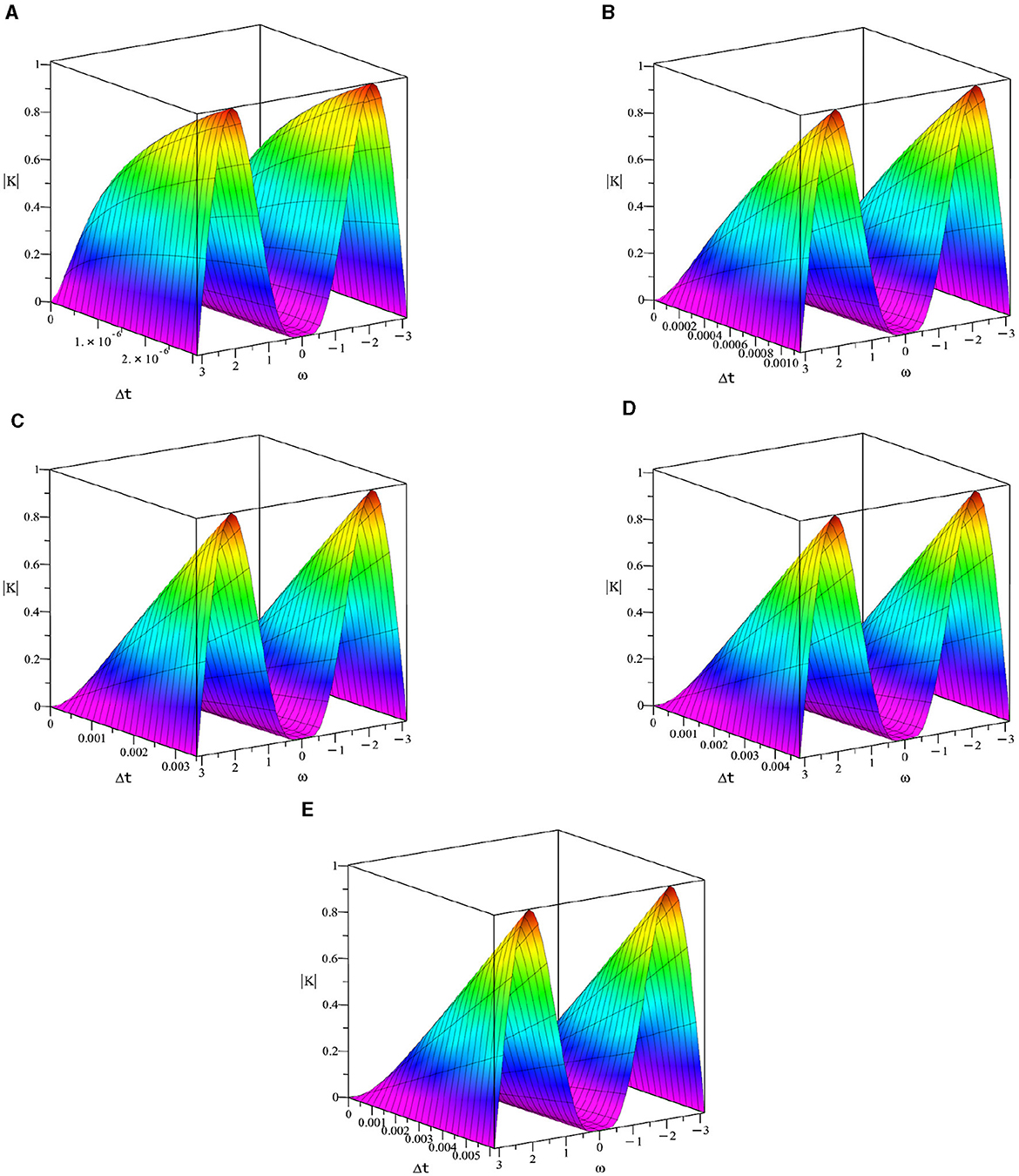
Figure 1. Plots of $\left|\mathcal{K}\right|$ vs. ω ∈ [−π, π] vs. Δt when $\mathrm{\Delta }x=\frac{\pi }{10}$ at some values of α in order to determine range of Δt for stability. (A) α = 0.40. (B) α = 0.75. (C) α = 0.90. (D) α = 0.95. (E) α = 1.0.

TABLE 1

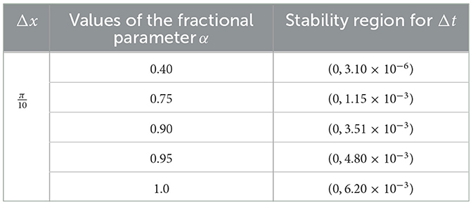
Table 1. Range of values of Δt for stability of FDMCO scheme at some values of α.

We can see from Table 1 that the stability region becomes more restricted as α is decreased from 1.0.

4.3 Consistency

We apply Taylor series expansion about (t_n, x_j) to the discretized scheme in Equation (10) to obtain

$\begin{array}{l}U+(\mathrm{\Delta }t)U_t+\frac{{(\mathrm{\Delta }t)}^2}{2}{U}_{tt}+\frac{{(\mathrm{\Delta }t)}^3}{6}{U}_{ttt}+\mathcal{O}((\mathrm{\Delta }t{)}^4)\\ =U-(\mathrm{\Delta }t)U_t+\frac{{(\mathrm{\Delta }t)}^2}{2}{U}_{tt}-\frac{{(\mathrm{\Delta }t)}^3}{6}{U}_{ttt}+\mathcal{O}((\mathrm{\Delta }t{)}^4)\\ -\frac{{(\mathrm{\Delta }t)}^{\alpha }}{\mathrm{\Delta }x}[U+(\mathrm{\Delta }x)U_x+\frac{{(\mathrm{\Delta }x)}^2}{2!}{U}_{xx}+\frac{{(\mathrm{\Delta }x)}^3}{3!}{U}_{xxx}\\ -\left(U-(\mathrm{\Delta }x)U_x+\frac{{(\mathrm{\Delta }x)}^2}{2!}{U}_{xx}-\frac{{(\mathrm{\Delta }x)}^3}{3!}{U}_{xxx}\right)+\mathrm{...}]\\ -\frac{{(\mathrm{\Delta }t)}^{\alpha }}{{(\mathrm{\Delta }x)}^3}[(U+2(\mathrm{\Delta }x)U_x+\frac{{(2\mathrm{\Delta }x)}^2}{2}{U}_{xx}+\frac{{(2\mathrm{\Delta }x)}^3}{3!}{U}_{xxx}\\ +\frac{{(2\mathrm{\Delta }x)}^4}{4!}{U}_{xxxx}+\mathcal{O}((\mathrm{\Delta }x{)}^5))-2(U+(\mathrm{\Delta }x)U_x+\frac{{(\mathrm{\Delta }x)}^2}{2!}{U}_{xx}\\ +\frac{{(\mathrm{\Delta }x)}^3}{3!}{U}_{xxx}+\frac{{(\mathrm{\Delta }x)}^4}{4!}{U}_{xxxx}+\mathcal{O}((\mathrm{\Delta }x{)}^5))\\ +2(U-(\mathrm{\Delta }x)U_x+\frac{{(\mathrm{\Delta }x)}^2}{2!}{U}_{xx}-\frac{{(\mathrm{\Delta }x)}^3}{3!}{U}_{xxx}+\\ \frac{{(\mathrm{\Delta }x)}^4}{4!}{U}_{xxxx}+\mathcal{O}((\mathrm{\Delta }x{)}^5))-(U-2(\mathrm{\Delta }x)U_x+\frac{{(2(\mathrm{\Delta }x))}^2}{2!}{U}_{xx}\\ -\frac{{(2(\mathrm{\Delta }x))}^3}{3!}{U}_{xxx}+\frac{{(2(\mathrm{\Delta }x))}^4}{4!}{U}_{xxxx}+\mathcal{O}((\mathrm{\Delta }x{)}^5)]\\ +4·(\mathrm{\Delta }t{)}^{\alpha }·t_n\cos (x_j),\end{array}$

which gives

$\begin{array}{l}\begin{array}{l}\frac{\partial U}{\partial t}+\frac{{(\mathrm{\Delta }t)}^{\alpha }}{\mathrm{\Delta }t}{U}_x+\frac{{(\mathrm{\Delta }t)}^{\alpha }}{\mathrm{\Delta }t}{U}_{xxx}-2\frac{{(\mathrm{\Delta }t)}^{\alpha }}{\mathrm{\Delta }t}{t}_n\cos (x_j)\hfill \end{array}\\ =-\frac{1}{3!}(\mathrm{\Delta }t{)}^2{U}_{ttt}-\frac{1}{3!}(\mathrm{\Delta }x{)}^2\frac{{(\mathrm{\Delta }t)}^{\alpha }}{\mathrm{\Delta }t}{U}_{xxx}+\mathcal{O}((\mathrm{\Delta }x{)}^2).& (18)\end{array}$

If we multiply both sides of Equation (18) by (Δt)^1−α, we obtain

$\begin{array}{l}\frac{{\partial }^{\alpha }U}{\partial t^{\alpha }}+\frac{\partial U}{\partial x}+\frac{{\partial }^{3}U}{\partial t^3}-2t_n\cos (x_j)\\ =-\frac{{(\mathrm{\Delta }t)}^{3-\alpha }}{3!}{U}_{ttt}-\frac{{(\mathrm{\Delta }x)}^2}{3!}{U}_{xxx}+\mathcal{O}\left({(\mathrm{\Delta }x)}^2{(\mathrm{\Delta }t)}^{1-\alpha }\right).& (19)\end{array}$

Thus, the FDMCO scheme is consistent with the PDE in Equation (1) and is accurate of order (3−α) in time and accurate of order 2 in space.

5 Numerical results from FDMCO

5.1 Display of L₁ and L_∞ errors

We present in Tables 2–6, the L₁ and L_∞ errors at the three different times and some different values of Δt for the five cases: α = 0.40, 0.75, 0.90, 0.95, and 1.0. We note that in all numerical experiments, we chose $\mathrm{\Delta }x=\frac{\pi }{10}.$ The values of Δt are chosen from the range of values of Δt for which the scheme is stable as explained in Table 1.

TABLE 2

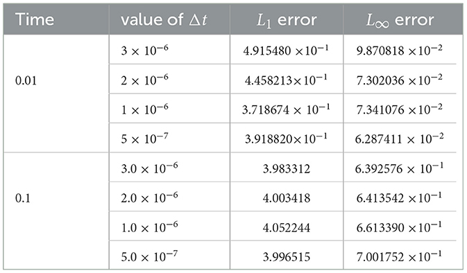
Table 2. L₁ and L_∞ errors using $\mathrm{\Delta }x=\frac{\pi }{10}$ when α = 0.40 at different values of time.

TABLE 3

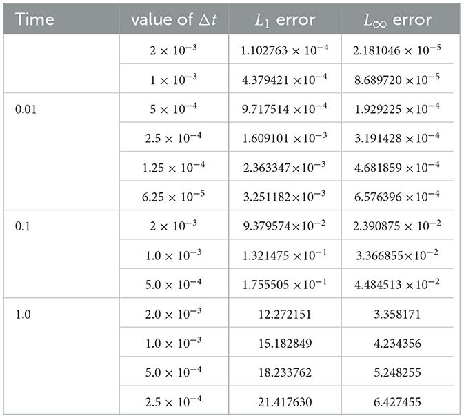
Table 3. L₁ and L_∞ errors using $\mathrm{\Delta }x=\frac{\pi }{10}$ when α = 0.75 at different values of time.

TABLE 4

Table 4. L₁ and L_∞ errors using $\mathrm{\Delta }x=\frac{\pi }{10}$ when α = 0.90 at different values of time.

TABLE 5

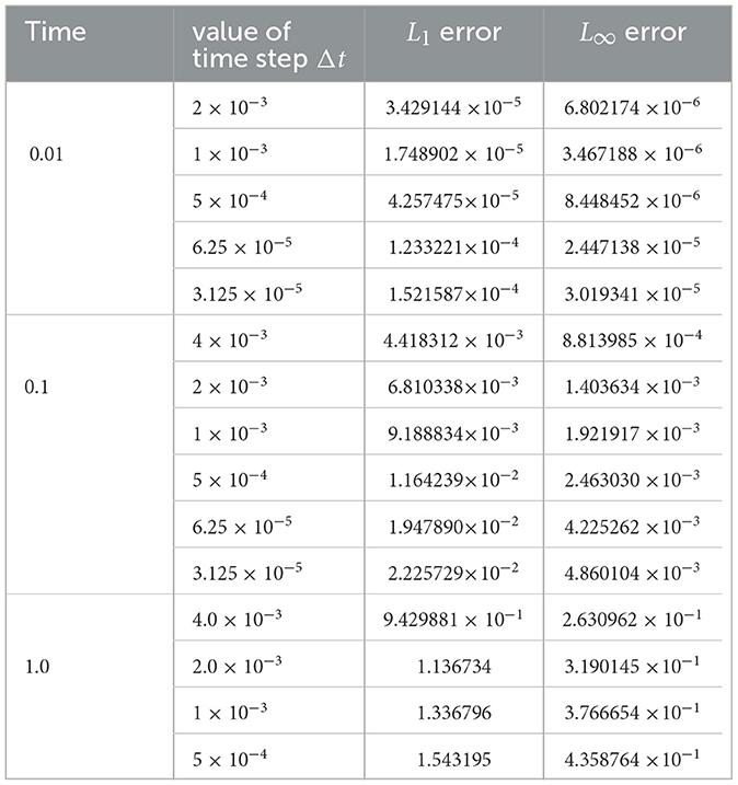
Table 5. L₁ and L_∞ errors using $\mathrm{\Delta }x=\frac{\pi }{10}$ when α = 0.95 at different values of time.

TABLE 6

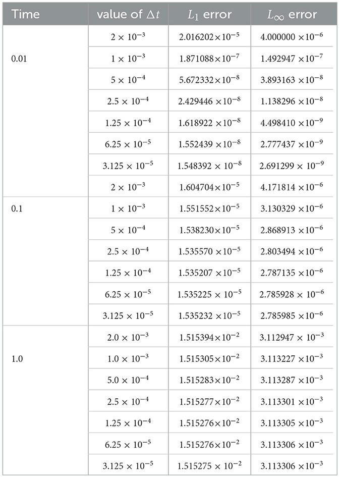
Table 6. L₁ and L_∞ errors using $\mathrm{\Delta }x=\frac{\pi }{10}$ when α = 1.0 at different values of time.

We can see from Tables 5, 6 that FDMCO scheme performs well for the considered experiment for α = 0.95, 1.0, respectively, at time 0.01, 0.1. The FDMCO scheme performs quite well at time 1.0 only for the case when α = 1.0.

5.2 Numerical profiles and relative errors: FDMCO

We plot numerical solutions vs. x for five α values at times 0.01, 0.1,, and 1.0 using the optimal Δt.

Figure 2 illustrates 2D plots of the numerical solution vs. x at time 0.01. Figure 3 presents graphs of the numerical solution with respect to x at time 0.1.

FIGURE 2

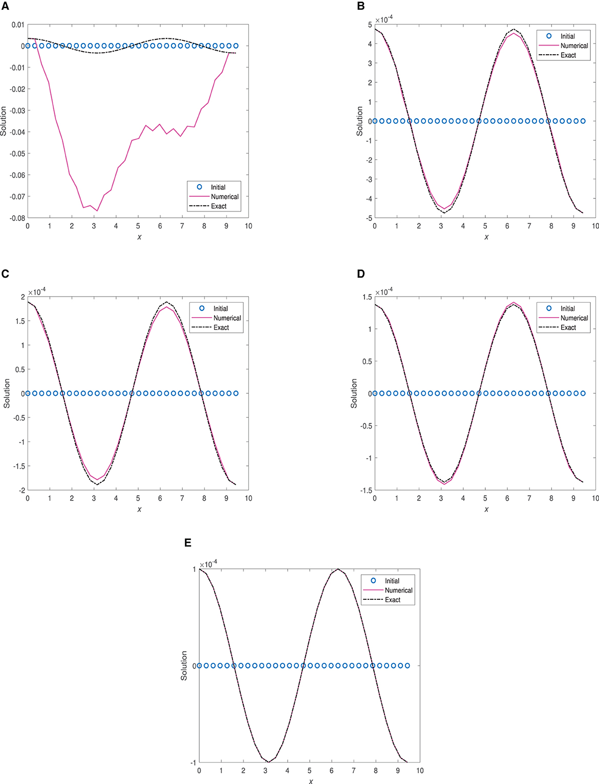
Figure 2. Plots of numerical solution vs. x at time 0.01 using $\mathrm{\Delta }x=\frac{\pi }{10}$ and optimal Δt. (A) α = 0.40, Δt = 1.0 × 10⁻⁶. (B) α = 0.75, Δt = 2.0 × 10⁻³. (C) α = 0.90, Δt = 2.0 × 10⁻³. (D) α = 0.95, Δt = 1.0 × 10⁻³. (E) α = 1.0, Δt = 3.125 × 10⁻⁵.

FIGURE 3

Figure 3. Plots of numerical solution vs. x at time 0.1 using $\mathrm{\Delta }x=\frac{\pi }{10}$ and optimal Δt. (A) α = 0.75, Δt = 2.0 × 10⁻³. (B) α = 0.90, Δt = 4.0 × 10⁻³. (C) α = 0.95, Δt = 4.0 × 10⁻³. (D) α = 1.0, Δt = 6.25 × 10⁻⁵.

Figure 4 demonstrates plots of the numerical solution vs. x at time 1.0. The computations utilized $\mathrm{\Delta }x=\frac{\pi }{10}$ and the optimal Δt for fractional parameters α = 0.40, 0.75, 0.90, 0.95, 1.0.

FIGURE 4

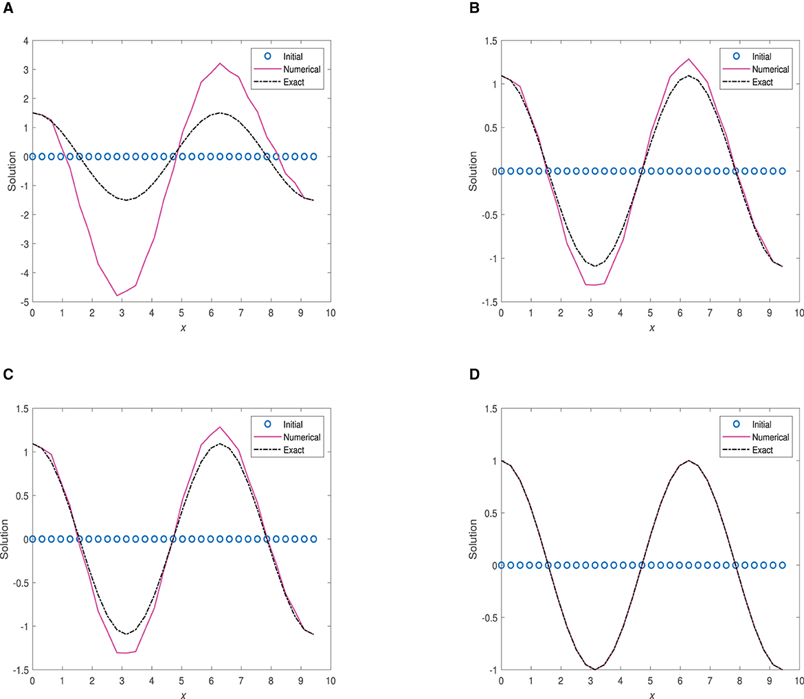
Figure 4. Plots of numerical solution vs. x at time 1.0 using $\mathrm{\Delta }x=\frac{\pi }{10}$ and optimal Δt. (A) α = 0.75, Δt = 2.0 × 10⁻³. (B) α = 0.90, Δt = 4.0 × 10⁻³. (C) α = 0.95, Δt = 4.0 × 10⁻³. (D) α = 1.0, Δt = 3.125 × 10⁻⁵.

Additionally, Figures 5–7 display graphs of the relative errors with respect to x at the three different time values.

FIGURE 5

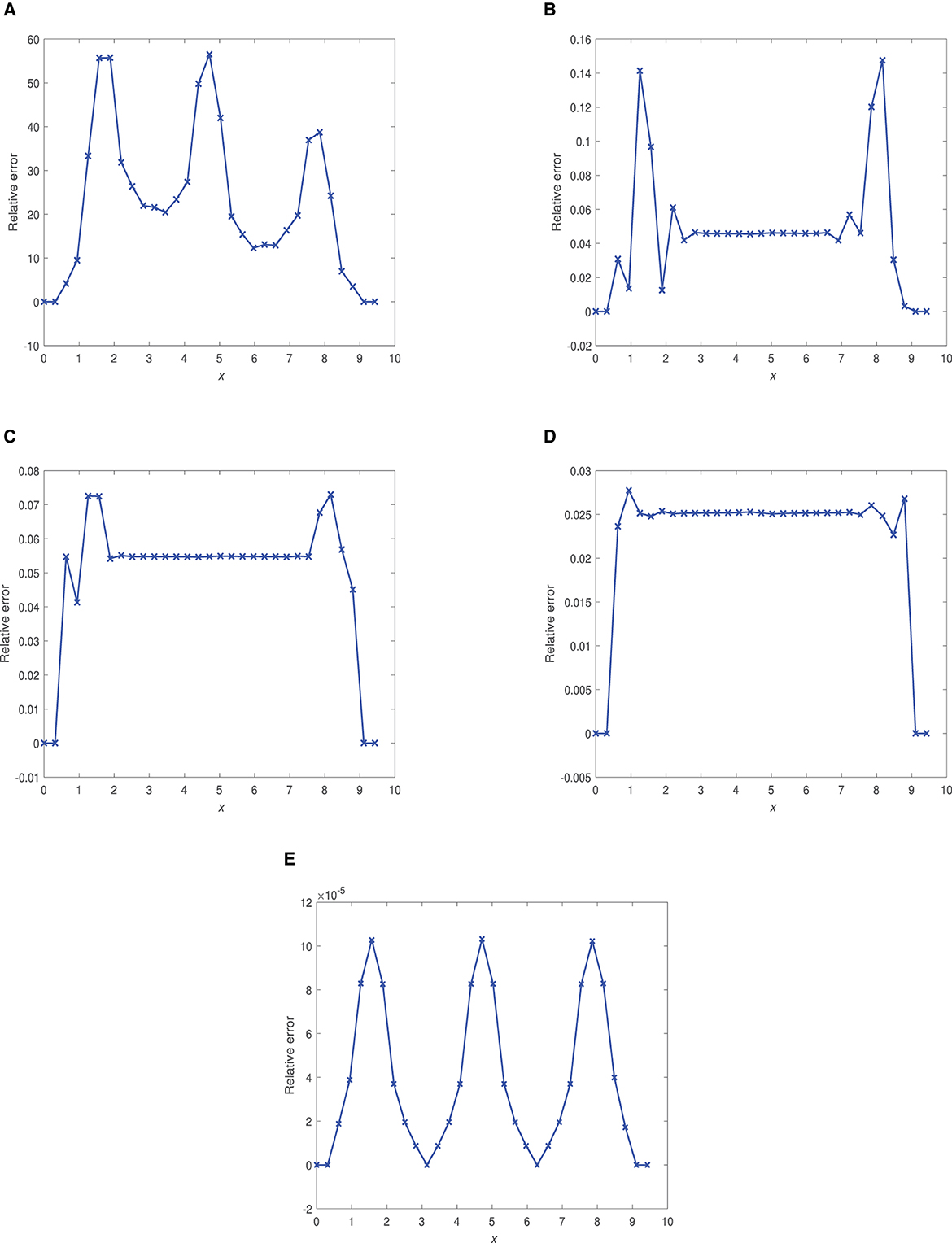
Figure 5. Plots of relative errors vs. x at time 0.01 using $\mathrm{\Delta }x=\frac{\pi }{10}$ and optimal Δt. (A) α = 0.40, Δt = 1.0 × 10⁻⁶. (B) α = 0.75, Δt = 2.0 × 10⁻³. (C) α = 0.90, Δt = 2.0 × 10⁻³. (D) α = 0.95, Δt = 1.0 × 10⁻³. (E) α = 1.0, Δt = 3.125 × 10⁻⁵.

FIGURE 6

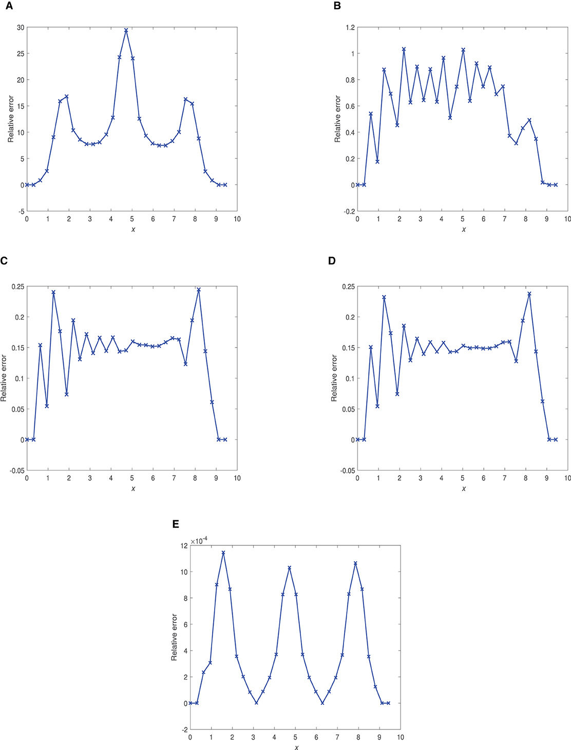
Figure 6. Plots of relative errors vs. x at time 0.1 using $\mathrm{\Delta }x=\frac{\pi }{10}$ and optimal Δt. (A) α = 0.40, Δt = 1.0 × 10⁻⁶. (B) α = 0.75, Δt = 2.0 × 10⁻³. (C) α = 0.90, Δt = 4.0 × 10⁻³. (D) α = 0.95, Δt = 1.0 × 10⁻³. (E) α = 1.0, Δt = 3.125 × 10⁻⁵.

FIGURE 7

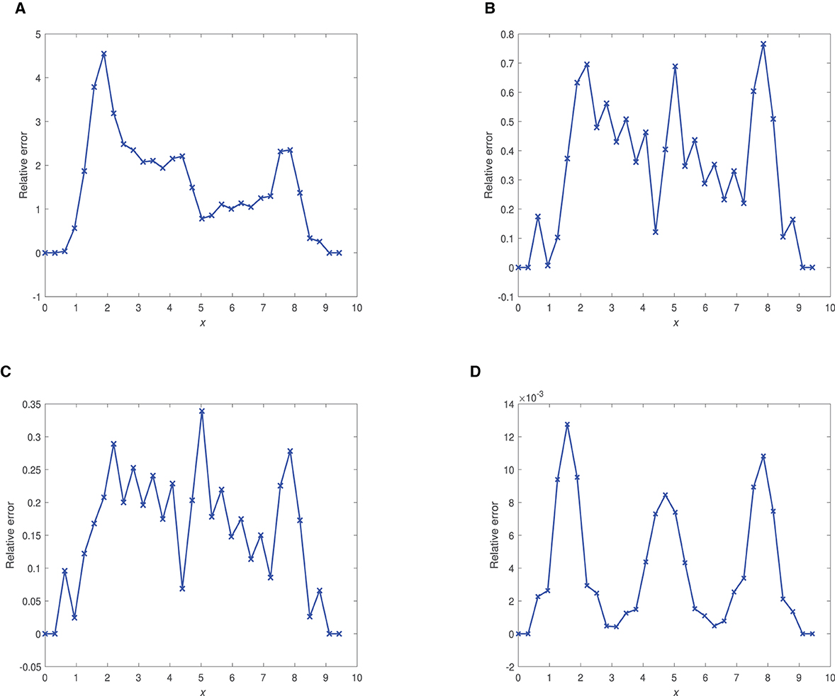
Figure 7. Plots of relative errors vs. x at time 1.0 using $\mathrm{\Delta }x=\frac{\pi }{10}$ and optimal Δt. (A) α = 0.75, Δt = 2.0 × 10⁻³. (B) α = 0.90, Δt = 4.0 × 10⁻³. (C) α = 0.95, Δt = 4.0 × 10⁻³. (D) α = 1.0, Δt = 3.125 × 10⁻⁵.

Figure 5 depicts graphs for the relative errors vs. x at time 0.01 using the FDMCO scheme with $\mathrm{\Delta }x=\frac{\pi }{10}$ and optimal Δt for five different fractional parameters α = 0.40, 0, 75, 0.90, 0.95, 1.0. We have plotted the relative error by ignoring three nodal points ($x=\frac{\pi }{2}=1.571,\frac{3\pi }{2}=4.712,\frac{5\pi }{2}=7.854$) as the exact solution at these points lies in the range 10⁻²² to 10⁻⁴ (very close to zero) for the five different values of the fractional parameter α.

Corresponding plots of relative errors vs. x at time 0.1 and 1.0 are shown in Figures 6, 7.

5.3 Discussion of results: FDMCO

At α = 0.40 and time 0.01, the scheme exhibits poor performance, with the L₁ error of order 10⁻¹. As time increases to 0.1, the scheme's performance worsens, and the L_∞ error follows a similar trend, ranging from approximately 10⁻² to 10⁻¹.

At α = 0.75 and time 0.01, the scheme performs quite well, with the L₁ error at 10⁻⁴ and the L_∞ error ranging from 10⁻⁵ to 10⁻⁴. However, when the time is increased to 0.1, the L₁ errors increase to approximately 10⁻² up to 10⁻¹. The optimal step size appears to be 2 × 10⁻³ as indicated in Table 3.

At α = 0.90 and time 0.01, the FDMCO scheme produces very good results, with L₁ errors of order 10⁻⁵ and 10⁻⁴. The L₁ errors are of order 10⁻² at time 0.1. The L_∞ error also exhibits some variation, ranging from 10⁻⁵ to 10⁻¹ for all three time values t = 0.01, 0.1, 1.0.

At α = 0.95, the scheme performs very well at time 0.01, and quite well at time 0.1. Quite satisfactorily results are obtained at time 0.1 when Δt = 4.0 × 10⁻³.

We have different behavior of FDMCO scheme at α = 1.0. Good performance at all the times 0.01, 0.1,, and 1.0. The general trend is as Δt decreases, the L₁ error decreases at the three different values of time. The L_∞ error follows a similar trend, with errors ranging from approximately 10⁻⁹ to 10⁻³.

In summary, the scheme's performance relies on the value of the fractional parameter α and the chosen time step Δt. Overall, the FDMCO scheme demonstrates considerable effectiveness for fractional parameter values that are close to 1.0.

As referred to in Section 2, we notice that

Based on Figures 5–7, we observe that:

(i) FDMCO gives satisfactory performance at α = 0.40 and time 0.01 with maximum relative error being 14%.

(ii) FDMCO is deemed satisfactory when α = 0.95, time = 0.1 (with maximum relative error being 23.5%) and when α = 0.90, time = 0.1 (with maximum relative error being about 23%).

(iii) FDMCO is highly effective at α = 1.0 for the three times: 0.01, 0.1, and 1.0.

6 Finite difference method using Caputo derivative (FDMCA)

To numerically solve this equation, we employ an explicit finite difference scheme with Caputo's approximation. The scheme to be constructed needs discretizing both spatial and time derivatives using central differences and incorporates the Caputo derivative with its L1 approximation [3].

Murio [35] derived an implicit scheme for a time-fractional diffusion equation. He approximated $\frac{{\partial }^{\alpha }u}{\partial t^{\alpha }}$ as follows:

$\begin{array}{l}\frac{{\partial }^{\alpha }u(x_j,t_n)}{\partial t^{\alpha }}=\frac{1}{\mathrm{\Gamma }(1-\alpha )}{\displaystyle {\int }_0^{t_n}\frac{\partial u(x_j,t)}{\partial t}}\frac{1}{{\left(t_n-t\right)}^{\alpha }}\text{d}t\\ =\frac{1}{\mathrm{\Gamma }(1-\alpha )}{\displaystyle \sum _{i=1}^n{\displaystyle {\int }_{(i-1)k}^{ik}\left[\frac{U_j^i-U_j^{i-1}}{k}+\Theta (k)\right]}}{\left(nk-t\right)}^{-\alpha }\text{d}t\\ =\frac{1}{\mathrm{\Gamma }(1-\alpha )}{\displaystyle \sum _{i=1}^n\left\{\left(\frac{U_j^i-U_j^{i-1}}{k}\right){[\frac{{(nk-t)}^{-\alpha +1}}{-(1-\alpha )}]}_{t=(i-1)k}^{t=ik}\right\}}\\ +\frac{1}{\mathrm{\Gamma }(1-\alpha )}{\displaystyle \sum _{i=1}^n\{}[\frac{{(nk-t)}^{-\alpha +1}}{-(1-\alpha )}{]}_{t=(i-1)k}^{t=ik}\}·\Theta (k),\\ =\frac{1}{\mathrm{\Gamma }(1-\alpha )}{\displaystyle \sum _{i=1}^n\{\left(\frac{U_j^i-U_j^{i-1}}{k}\right)[\frac{{(nk-ik)}^{-\alpha +1}}{-(1-\alpha )}}\\ +\frac{{(nk-ik+k)}^{-\alpha +1}}{(1-\alpha )}{]}_{t=(i-1)k}^{t=ik}\}\\ +\frac{1}{\mathrm{\Gamma }(1-\alpha )}{\displaystyle \sum _{i=1}^n\{[\frac{{(nk-ik)}^{-\alpha +1}}{-(1-\alpha )}}\\ +\frac{{(nk-ik+k)}^{-\alpha +1}}{(1-\alpha )}{]}_{t=(i-1)k}^{t=ik}\}·\Theta (k),\\ =\frac{1}{\mathrm{\Gamma }(1-\alpha )}{\displaystyle \sum _{i=1}^n\{\left(\frac{U_j^i-U_j^{i-1}}{k}\right)·k^{1-\alpha }}\\ ·{[\frac{{\left(n-i+1\right)}^{1-\alpha }-{\left(n-i\right)}^{1-\alpha }}{-(1-\alpha )}]}_{t=(i-1)k}^{t=ik}\}\\ +\frac{1}{\mathrm{\Gamma }(1-\alpha )}{\displaystyle \sum _{i=1}^n[}\frac{{\left(n-i+1\right)}^{1-\alpha }-{\left(n-i\right)}^{1-\alpha }}{-(1-\alpha )}{]}_{t=(i-1)k}^{t=ik}\\ ·\Theta (k^{2-\alpha }).\end{array}$

For simplification, the formula Γ(2−α) = (1−α)Γ(1−α) is used.

$\begin{array}{l}\frac{{\partial }^{\alpha }u(x_j,t_n)}{\partial t^{\alpha }}\simeq \frac{k^{-\alpha }}{\mathrm{\Gamma }(2-\alpha )}{\displaystyle \sum _{i=1}^n\{\left(U_j^i-U_j^{i-1}\right)}\\ ·[{\left(n-i+1\right)}^{1-\alpha }-{\left(n-i\right)}^{1-\alpha }].\end{array}$

This discretization gives rise to an implicit scheme. We attempt to discretize $\frac{{\partial }^{\alpha }u(x_j,t_n)}{\partial t^{\alpha }}$ to construct an explicit scheme to solve the fractional KdV equation. We approximate $\frac{\partial u(x,t)}{\partial t}$ by $\frac{U_j^{i+1}-U_j^i}{k}$

$\begin{array}{l}\frac{{\partial }^{\alpha }u(x_j,t_n)}{\partial t^{\alpha }}=\frac{1}{(1-\alpha )}{\displaystyle {\int }_0^{t_n}\frac{\partial u(x_j,\tau )}{\partial \tau }}(t_n-\tau {)}^{-\alpha }\text{d}\tau ,\text{ where }{t}_n=nk,\\ =\frac{1}{\mathrm{\Gamma }(1-\alpha )}{\displaystyle \sum }_{i=1}^n\left\{{\displaystyle {\int }_{(i-1)k}^{ik}\left[\frac{U_j^{i+1}-U_j^i}{k}+\Theta (k)\right]}{\left(nk-\tau \right)}^{-\alpha }\text{d}\tau \right\}\\ =\frac{1}{\mathrm{\Gamma }(1-\alpha )}{\displaystyle \sum _{i=1}^n\{}\left[\frac{U_j^{i+1}-U_j^i}{k}+\Theta (k)\right]{\displaystyle {\int }_{(i-1)k}^{ik}{\left(nk-\tau \right)}^{-\alpha }}\text{d}\tau \}\\ =\frac{1}{\mathrm{\Gamma }(1-\alpha )}{\displaystyle \sum _{i=1}^n\{}\left(\frac{U_j^{i+1}-U_j^i}{k}+\Theta (k)\right)[\frac{-{(nk-t)}^{-\alpha +1}}{(1-\alpha )}{]}_{t=(i-1)k}^{t=ik}\}\\ =\frac{1}{\mathrm{\Gamma }(1-\alpha )}{\displaystyle \sum _{i=1}^n\{}\left(\frac{U_j^{i+1}-U_j^i}{k}+\Theta (k)\right)[\frac{-{(nk-t)}^{-\alpha +1}}{(1-\alpha )}{]}_{t=(i-1)k}^{t=ik}\}\\ =\frac{k^{1-\alpha }}{(1-\alpha )\mathrm{\Gamma }(1-\alpha )}{\displaystyle \sum _{i=1}^n\left(\frac{U_j^{i+1}-U_j^i}{k}+\Theta (k)\right)}\\ ·[{\left(n-i+1\right)}^{1-\alpha }-{\left(n-i\right)}^{1-\alpha }]\\ =\frac{1}{(1-\alpha )\mathrm{\Gamma }(1-\alpha )}{\displaystyle \sum _{i=1}^n\{}\left(\frac{U_j^{i+1}-U_j^i}{k^{\alpha }}+\Theta (k^{2-\alpha })\right)\\ ·[{\left(n-i+1\right)}^{1-\alpha }-{\left(n-i\right)}^{1-\alpha }]\}\\ \simeq \frac{1}{\mathrm{\Gamma }(2-\alpha )}{k}^{-\alpha }{\displaystyle \sum _{i=1}^n\left(U_j^{i+1}-U_j^i\right)}·[{\left(n-i+1\right)}^{1-\alpha }-{\left(n-i\right)}^{1-\alpha }].& (20)\end{array}$

We note that

$\begin{array}{l}{\displaystyle \sum _{i=1}^n\left(U_j^{i+1}-U_j^i\right)}·[{\left(n-i+1\right)}^{1-\alpha }-{\left(n-i\right)}^{1-\alpha }]\\ =\left(U_j^2-U_j^1\right)\left(n^{1-\alpha }-{(n-1)}^{1-\alpha }\right)\\ +\left(U_j^3-U_j^2\right){\left({(n-1)}^{1-\alpha }-(n-2)\right)}^{1-\alpha }\\ +\left(U_j^4-U_j^3\right)\left({(n-2)}^{1-\alpha }-{(n-3)}^{1-\alpha }\right)\\ +\left(U_j^5-U_j^4\right)\left({(n-3)}^{1-\alpha }-{(n-4)}^{1-\alpha }\right)\\ +\cdots +\left(U_j^n-U_j^{n-1}\right)\left(2^{1-\alpha }-1^{1-\alpha }\right)\\ +\left(U_j^{n+1}-U_j^n\right)\left(1^{1-\alpha }-0\right),\end{array}$

which can be written as

$\begin{array}{l}{U}_j^{n+1}-U_j^n+{\displaystyle \sum _{i=1}^{n-1}}\left[{(i+1)}^{1-\alpha }-i^{1-\alpha }\right]\left(U_j^{n-i+1}-U_j^{n-i}\right).\end{array}$

Hence,

$\begin{array}{l}\frac{{\partial }^{\alpha }u(x_j,t_n)}{\partial t^{\alpha }}\simeq \frac{1}{\mathrm{\Gamma }(2-\alpha )}\frac{1}{k^{\alpha }}\{U_j^{n+1}-U_j^n\\ +{\displaystyle \sum _{i=1}^{n-1}\left(U_j^{n-i+1}-U_j^{n-i}\right)}\left[{(i+1)}^{1-\alpha }-i^{1-\alpha }\right]\}.& (21)\end{array}$

6.1 Derivation of FDMCA scheme

FDMCA when used to discrete Equation (1) is given by

$\begin{array}{l}\frac{k^{-\alpha }}{\mathrm{\Gamma }(2-\alpha )}\left(U_j^{n+1}-U_j^n\right)\\ +\frac{k^{-\alpha }}{\mathrm{\Gamma }(2-\alpha )}{\displaystyle \sum _{i=1}^{n-1}\left(U_j^{n-i+1}-U_j^{n-i}\right)}\left[{(i+1)}^{1-\alpha }-i^{1-\alpha }\right]\}& (22)\end{array}$

$\begin{array}{ll}+\frac{U_{j+1}^n-U_{j-1}^n}{2·(\mathrm{\Delta }x)}+\frac{U_{j+2}^n-2U_{j+1}^n+2U_{j-1}^n-2U_{j-2}^n}{2·{(\mathrm{\Delta }x)}^3}=2t_{n}cos(x_j).& (23)\end{array}$

We therefore have

$\begin{array}{l}{U}_j^{n+1}=U_j^n-\frac{k^{-\alpha }}{\mathrm{\Gamma }(2-\alpha )}{\displaystyle \sum _{i=1}^{n-1}\left(U_j^{n-i+1}-U_j^{n-i}\right)}\left[{(i+1)}^{1-\alpha }-i^{1-\alpha }\right]\}\\ -\frac{U_{j+1}^n-U_{j-1}^n}{2·(\mathrm{\Delta }x)}·k^{\alpha }·\mathrm{\Gamma }(2-\alpha )\\ -\frac{\mathrm{\Gamma }(2-\alpha )·k^{\alpha }}{2·{(\mathrm{\Delta }x)}^3}\left(U_{j+2}^n-2U_{j+1}^n+2U_{j-1}^n-2U_{j-2}^n\right)& (24)\end{array}$

$\begin{array}{ll}+k^{\alpha }·\mathrm{\Gamma }(2-\alpha )2t_{n}cos(x_j).& (25)\end{array}$

6.2 Stability of FDMCA scheme

To study the stability of FDMCA scheme, we consider the following equation

$\begin{array}{l}{U}_j^{n+1}=U_j^n-{\displaystyle \sum _{i=1}^{n-1}\left(U_j^{n+1-i}-U_j^{n-i}\right)}\left({(i+1)}^{1-\alpha }-i^{1-\alpha }\right)\\ -\left(\frac{U_{j+1}^n-U_{j-1}^n}{2·(\mathrm{\Delta }x)}\right)·k^{\alpha }·\mathrm{\Gamma }(2-\alpha )\\ -\frac{\mathrm{\Gamma }(2-\alpha )·k^{\alpha }}{2·{(\mathrm{\Delta }x)}^3}\left(U_{j+2}^n-2U_{j+1}^n+2U_{j-1}^n-2U_{j-2}^n\right).& (26)\end{array}$

We then substitute $U_j^n$ by ξⁿe^Ijω where ω = θh, where θ is the wave number and $I=\sqrt{-1}$. This gives

$\begin{array}{l}{\xi }^{n+1}{e}^{Ij\omega }={\xi }^n{e}^{Ij\omega }-{\displaystyle \sum _{i=1}^{n-1}{\xi }^{n+1-i}}\left(e^{Ij\omega }-{\xi }^{n-i}{e}^{Ij\omega }\right)·\left({(i+1)}^{1-\alpha }-i^{1-\alpha }\right)\\ -{\xi }^n{e}^{Ij\omega }\left(\frac{e^{I\omega }-e^{-I\omega }}{2·(\mathrm{\Delta }x)}\right)·\mathrm{\Gamma }(2-\alpha )·k^{\alpha }\\ -\frac{{\xi }^n·\mathrm{\Gamma }(2-\alpha )·k^{\alpha }}{2·{(\mathrm{\Delta }x)}^3}·e^{Ij\omega }·\left(e^{2I\omega }-2e^{I\omega }+2e^{-I\omega }-e^{-2I\omega }\right).\end{array}$

Upon simplification, we get

$\begin{array}{l}{\xi }^{n+1}={\xi }^n\{1-\frac{2I\sin (\omega )}{2h}·\mathrm{\Gamma }(2-\alpha )·k^{\alpha }\\ -\frac{\mathrm{\Gamma }(2-\alpha )}{2h^3}·\left(2I\sin (2\omega )-4I\sin (\omega )\right)& (27)\end{array}$

$\begin{array}{ll}-{\displaystyle \sum _{i=1}^{n-1}\left({\xi }^{n+1-i}-{\xi }^{n-i}\right)}\left({(i+1)}^{1-\alpha }-i^{1-\alpha }\right)\}.& (28)\end{array}$

(i) We take the case n = 1:

$\begin{array}{ll}\left|\xi \right|=\{1+[\frac{\sin (\omega )}{h}\mathrm{\Gamma }(2-\alpha )·k^{\alpha }+\frac{\mathrm{\Gamma }(2-\alpha )}{2h^3}·k^{\alpha }& (29)\end{array}$

$\begin{array}{ll}{{·\left(2\sin (2\omega )-4\sin (\omega )\right)]}^2\}}^{\frac{1}{2}}.& (30)\end{array}$

The scheme is unstable when n = 1.

(ii) For the case n = 2, we get a quadratic equation in ξ:

$\begin{array}{l}{\xi }^2+\xi (2^{1-\alpha }-B-1)-(2^{1-\alpha }-1)=0,\end{array}$

where

$\begin{array}{ll}B=1-\frac{Isin(\omega )}{h}·\mathrm{\Gamma }(2-\alpha )·k^{\alpha }-\frac{\mathrm{\Gamma }(2-\alpha )}{2h^3}& (31)\end{array}$

$\begin{array}{ll}·k^{\alpha }·(2Isin(2\omega )-4Isin(\omega )).& (32)\end{array}$

This gives

$\begin{array}{ll}{\xi }_{1,2}=\frac{B+1-2^{1-\alpha }\pm \sqrt{{(2^{1-\alpha }-B-1)}^2+4(2^{1-\alpha }-1)}}{2}.& (33)\end{array}$

We plot |ξ₁| vs. ω∈[−π, π] vs. k and |ξ₂| vs. ω∈[−π, π] vs. k for the five cases: α = 0.40, 0.75, 0.90, 0.95, 1.0.

It is seen that |ξ₂| < 1 for all values of k>0 and ω∈[−π, π]. However, |ξ₁|≥1 for k>0 and ω∈[−π, π].

We obtain some range of values of k for which scheme is mildly stable, in that case, we choose |ξ₁| ≤ 1.03 and the results are showed in Table 7.

TABLE 7

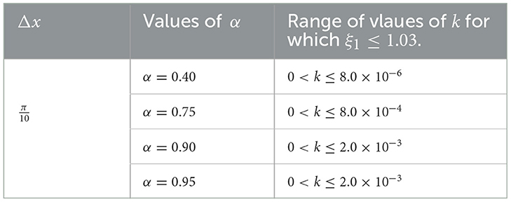
Table 7. Range of values of Δt for stability of FDMCA scheme at some values of α.

We see that as we increase n and keep α fixed, the stability limit for k increases. If we keep α fixed and increase n, the stability region for k is enlarged.

As n get larger, the expression for the amplification factor gets more complicated and stability analysis become difficult for the explicit FDMCA scheme. We plan in future to construct NSFD methods using Caputo approximations or construct implicit versions of FDMCA scheme.

Remark 1. We would like to point out that for the case when α = 1.0, the stability is straightforwardly established, similar to the classical KdV approach demonstrated in our previous studies in Appadu and Kelil [10] and Kelil [36].

7 Numerical results: FDMCA scheme

In this section, we present some numerical profiles for the FDMCA scheme to solve the non-homogeneous KdV equation. We now compute the accuracy of the numerical solution and also the performance of the scheme by computing L₁ and L_∞ errors. We compare the numerical solutions obtained by both schemes for Equation (1) with its exact solution. Numerical calculations are carried out by using Matlab and Maple 18 on an Intel@COre i5 2.30GHz with 8 GB RAM and 64- bit operating system (Windows 10).

7.1 Display of L₁ & L_∞ errors (FDMCA)

We present in Tables 8–12, the L₁ and L_∞ errors at different times and various Δt values for five specific cases: α values of 0.40, 0.75, 0.90, 0.95, and 1.0. It is noteworthy that for all our experiments, we chose $\mathrm{\Delta }x=\frac{\pi }{10}$ and appropriately chosen Δt to ensure feasible solution profiles, as revealed in Figures 8–12 for three values of time t = 0.01, 0.1, 1.0.

TABLE 8

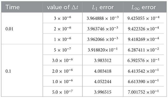
Table 8. L₁ and L_∞ errors using $\mathrm{\Delta }x=\frac{\pi }{10}$ when α = 0.40 at different values of time.

TABLE 9

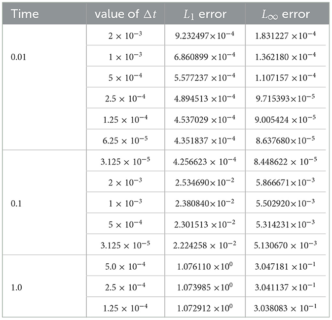
Table 9. L₁ and L_∞ errors using $\mathrm{\Delta }x=\frac{\pi }{10}$ when α = 0.75 at different values of time.

TABLE 10

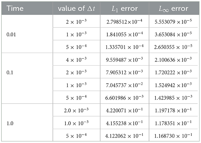
Table 10. L₁ and L_∞ errors using $\mathrm{\Delta }x=\frac{\pi }{10}$ when α = 0.90 at different values of time

TABLE 11

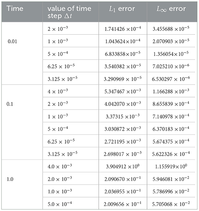
Table 11. L₁ and L_∞ errors using $\mathrm{\Delta }x=\frac{\pi }{10}$ when α = 0.95 at different values of time.

TABLE 12

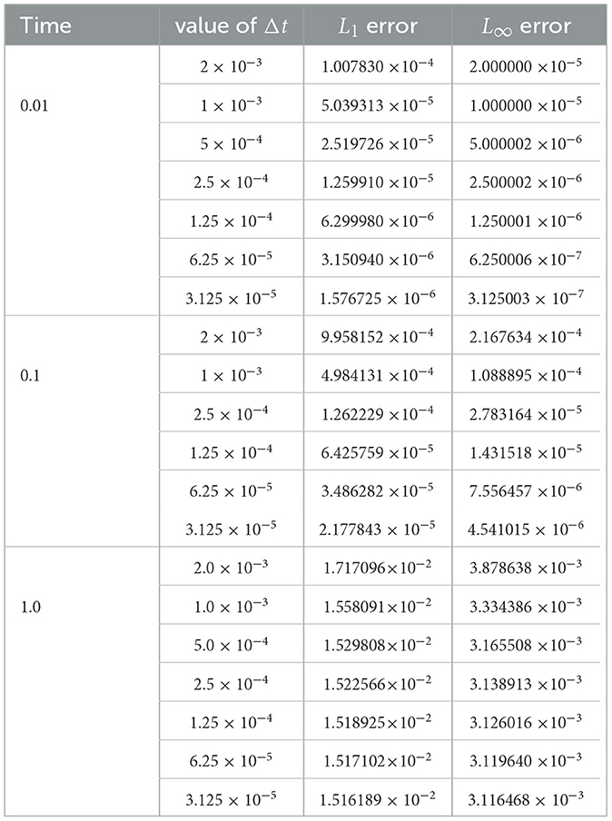
Table 12. L₁ and L_∞ errors using $\mathrm{\Delta }x=\frac{\pi }{10}$ when α = 1.0 at different values of time.

FIGURE 8

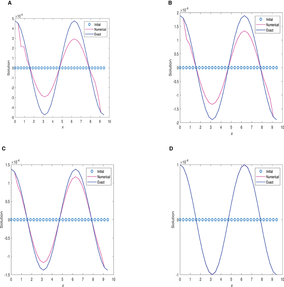
Figure 8. Plots of exact solution and solution using FDMCA vs. x at time = 0.01 and different values of α. (A) α = 0.75, Δt = 2.0 × 10⁻³. (B) α = 0.90, Δt = 2.0 × 10⁻³. (C) α = 0.95, Δt = 1.0 × 10⁻³. (D) α = 1.0, Δt = 3.125 × 10⁻⁵.

FIGURE 9

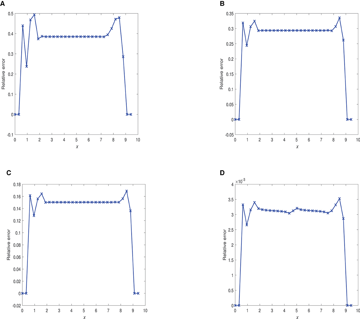
Figure 9. Plots of relative errors vs. x at time 0.01 using $\mathrm{\Delta }x=\frac{\pi }{10}$ and optimal Δt. (A) α = 0.75, Δt = 2.0 × 10⁻³. (B) α = 0.90, Δt = 2.0 × 10⁻³. (C) α = 0.95, Δt = 1.0 × 10⁻³. (D) α = 1.0, Δt = 3.125 × 10⁻⁵.

FIGURE 10

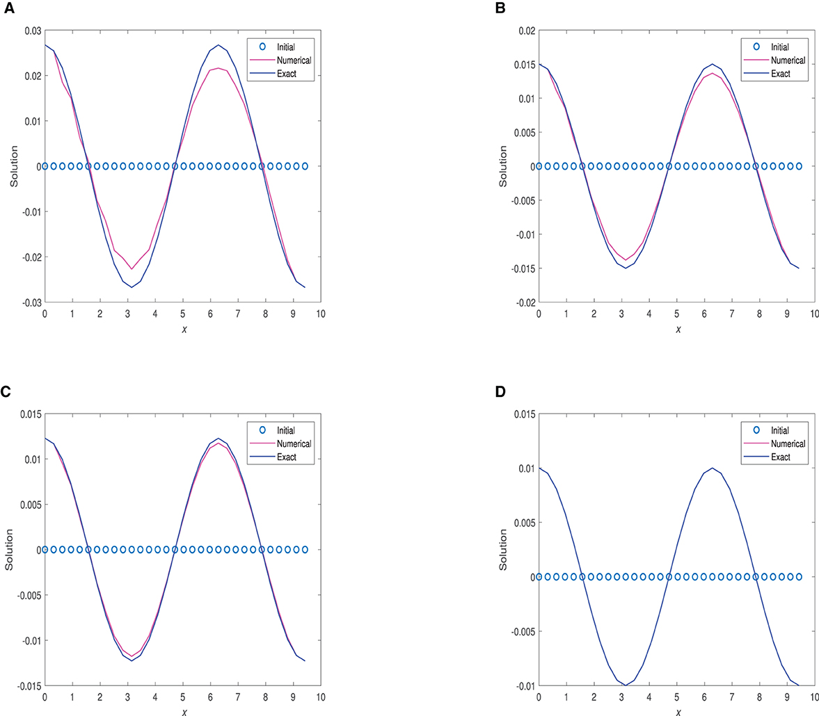
Figure 10. Plots of numerical solution vs. x at time 0.1 using $\mathrm{\Delta }x=\frac{\pi }{10}$ and optimal Δt. (A) α = 0.75, Δt = 3.125 × 10⁻⁵. (B) α = 0.95, Δt = 3.125 × 10⁻⁵. (C) α = 1.0, Δt = 3.125 × 10⁻⁵.

FIGURE 11

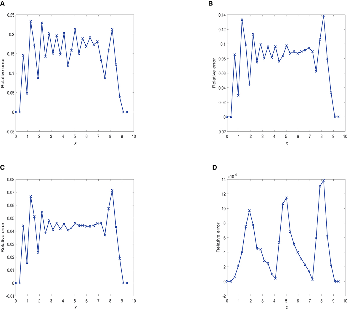
Figure 11. Plots of relative errors vs. x at time 0.1 using $\mathrm{\Delta }x=\frac{\pi }{10}$ and optimal Δt. (A) α = 0.75, Δt = 3.125 × 10⁻⁵. (B) α = 0.90, Δt = 5.0 × 10⁻⁴. (C) α = 0.95, Δt = 3.125 × 10⁻⁵. (D) α = 1.0, Δt = 3.125 × 10⁻⁵.

FIGURE 12

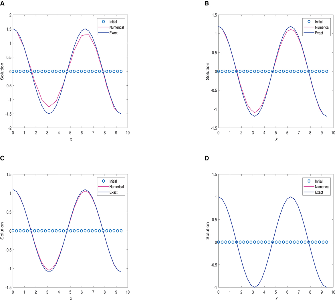
Figure 12. 2D plots of numerical solution vs. x at time 1.0 using $\mathrm{\Delta }x=\frac{\pi }{10}$ and optimal Δt. (A) α = 0.75, Δt = 1.25 × 10⁻⁴. (B) α = 0.90, Δt = 5.0 × 10⁻⁴. (C) α = 0.95, Δt = 5.0 × 10⁻⁴. (D) α = 1.0, Δt = 3.125 × 10⁻⁵.

FDMCA is much better than FDMCO at α = 0.40 for time 0.01. Moreover, FDMCA gives better results than FDMCO at α = 0.75, 0.90, 0.95 for all the three times 0.01, 0.1, 1.0.

7.2 Numerical profiles and relative errors: FDMCA

In this section, we present graphical comparisons of numerical solutions for x for five different α-values at three specific time points: 0.01, 0.1, and 1.0. These plots were generated using an appropriately selected Δt and a fixed grid spacing of $\mathrm{\Delta }x=\frac{\pi }{10}$.

Figure 8 displays 2D plots of the numerical solution at t = 0.01. Figure 10 shows numerical solution graphs at t = 0.1. Figure 12 demonstrates numerical solution plots at t = 1.0, utilizing α-values of 0.40, 0.75, 0.90, 0.95, and 1.0. Additionally, Figures 9, 11, 13 present graphs depicting the relative errors with respect to x for the FDMCA scheme at these three specific time points.

FIGURE 13

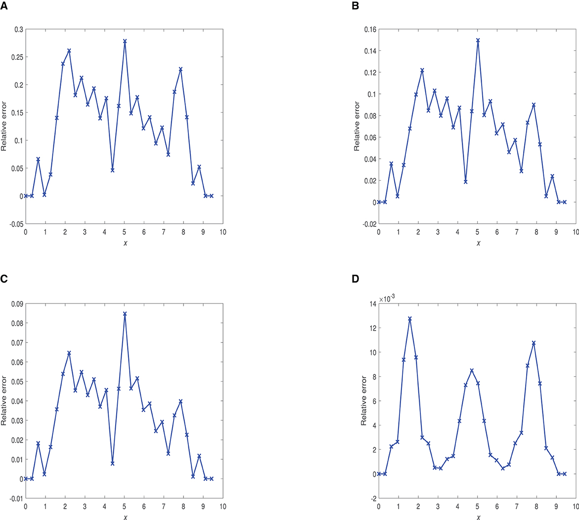
Figure 13. Plots of relative errors vs. x at time 1.0 using $\mathrm{\Delta }x=\frac{\pi }{10}$ and for some appropriately chosen optimal Δt. (A) α = 0.75, Δt = 1.25 × 10⁻⁴. (B) α = 0.90, Δt = 5.0 × 10⁻⁴. (C) α = 0.95, Δt = 5.0 × 10⁻⁴. (D) α = 1.0, Δt = 3.125 × 10⁻⁵.

At time 0.01, FDMCA is not effective at α = 0.75 and α = 0.90. However, the scheme gives satisfactory performance with maximum relative error being 18%. The scheme displays excellent performance when α = 1.0 with maximum relative error of 4.0 × 10⁻¹%.

FDMCA is highly effective at α = 0.95, α = 1.0 when time is 0.1 with maximum relative error being 8% and 14 × 10⁻²%, respectively. The scheme is deemed satisfactory at α = 0.75, α = 0.90 when time of propagation is 0.1.

FDMCA is highly effective at α = 0.95, α = 1.0 when time is 1.0 with maximum relative error being 8.5% and 13 × 10⁻¹%, respectively. The scheme is deemed satisfactory at α = 0.75, α = 0.90 when time of propagation is 1.0.

8 Conclusion

In this study, we have constructed two finite difference schemes to solve a non-homogeneous fractional dispersive Korteweg-de Vries (KdV) equation. We utilized both conformable and Caputo derivatives in our numerical methods and conducted a comprehensive analysis of their qualitative properties, including stability, consistency, and error analysis using both L₁ and L_∞ error norms. We presented tables and plots showing relative errors and provided graphical representations of numerical profiles for both schemes. When working with the FDMCO scheme, we observed the following scenarios at five different fractional papramter values α = 040, 0.75, 0.90, 0.95, 1.0 and at different times, including those as follows:

• At α = 0.75, 0.90, 0.95, 1.0 at time t = 0.01.

• At α = 0.90, 0.95, 1.0 at time t = 0.1.

• At α = 0.90, 0.95, 1.0 at time t = 1.0.

The FDMCA scheme yielded particularly good results for fractional values of α ranging from 0.75 up to 1.0, as evidenced by the tabulated data and accompanying figures. In general, the performance of both schemes is closely related to the fractional parameter α and the chosen time step Δt. We notice that both FDMCO and FDMCA schemes exhibit significant effectiveness, particularly when dealing with fractional parameter values that approach 1.0. When comparing the fractional parameter range α∈(0.40, 1.0], the FDMCA scheme outperforms the FDMCO scheme.

Data availability statement

The raw data supporting the conclusions of this article will be made available by the authors, without undue reservation.

Author contributions

AA: Conceptualization, Formal analysis, Investigation, Methodology, Project administration, Resources, Software, Supervision, Validation, Visualization, Writing – original draft, Writing – review & editing. AK: Formal analysis, Funding acquisition, Investigation, Methodology, Resources, Software, Validation, Visualization, Writing – original draft.

Funding

The author(s) declare financial support was received for the research, authorship, and/or publication of this article. AA is grateful to Nelson Mandela University, where the work was carried out. AK is grateful for postdoctoral research funding from NRF scarce skills fellowship under grant No. 138521.

Conflict of interest

The authors declare that the research was conducted in the absence of any commercial or financial relationships that could be construed as a potential conflict of interest.

Publisher's note

All claims expressed in this article are solely those of the authors and do not necessarily represent those of their affiliated organizations, or those of the publisher, the editors and the reviewers. Any product that may be evaluated in this article, or claim that may be made by its manufacturer, is not guaranteed or endorsed by the publisher.

References

1. Podlubny I. Fractional Differential Equations, Mathematics in Science and Engineering. New York: Academic press. (1999).

Google Scholar

2. Miller KS, Ross B. An Introduction to the Fractional Calculus and Fractional Differential Equations. New York: John Wiley and Sons. (1993).

Google Scholar

3. Oldham K, Spanier J. The Fractional Calculus Theory and Applications of Differentiation and Integration to Arbitrary Order. London: Elsevier. (1974).

Google Scholar

4. Podlubny I. Fractional Differential Equations: An Introduction to Fractional Derivatives, Fractional Differential Equations, to Methods of Their Solution and Some of Their Applications. London: Elsevier. (1998).

Google Scholar

5. Eriqat T, Oqielat MN, Al-Zhour Z, Khammash GS, El-Ajou A, Alrabaiah H. Exact and numerical solutions of higher-order fractional partial differential equations: a new analytical method and some applications. Pramana. (2022) 96:207. doi: 10.1007/s12043-022-02446-4

CrossRef Full Text | Google Scholar

6. Kordeweg D, de Vries G. On the change of form of long waves advancing in a rectangular channel, and a new type of long stationary wave. Philos Mag. (1895) 39:422–43. doi: 10.1080/14786449508620739

CrossRef Full Text | Google Scholar

7. Appadu AR, Kelil AS. On semi-analytical solutions for linearized dispersive KdV equations. Mathematics. (2020) 8:1769. doi: 10.3390/math8101769

CrossRef Full Text | Google Scholar

8. He JH. Homotopy perturbation technique. Comput Methods Appl Mech Eng. (1999) 178:257–62. doi: 10.1016/S0045-7825(99)00018-3

CrossRef Full Text | Google Scholar

9. Kelil AS, Appadu AR. On the numerical solution of 1D and 2D KdV equations using variational homotopy perturbation and finite difference methods. Mathematics. (2022) 10:4443. doi: 10.3390/math10234443

CrossRef Full Text | Google Scholar

10. Appadu AR, Kelil AS. Comparison of modified ADM and classical finite difference method for some third-order and fifth-order KdV equations. Demonstr Mathem. (2021) 54:377–409. doi: 10.1515/dema-2021-0039

CrossRef Full Text | Google Scholar

11. Sewell G. Analysis of a Finite Element Method: PDE/PROTRAN. Cham: Springer Science & Business Media. (2012).

Google Scholar

12. Aderogba AA, Appadu AR. Classical and multisymplectic schemes for linearized KdV equation: numerical results and dispersion analysis. Fluids. (2021) 6:214. doi: 10.3390/fluids6060214

CrossRef Full Text | Google Scholar

13. Rostamy D, Alipour M, Jafari H, Baleanu D. Solving multi-term orders fractional differential equations by operational matrices of BPs with convergence analysis. Rom Rep Phys. (2013) 65:334–49.

Google Scholar

14. Anwar A, Jarad F, Baleanu D, Ayaz F. Fractional Caputo heat equation within the double Laplace transform. Rom J Phys. (2013) 58:15–22.

Google Scholar

15. Jumarie G. Table of some basic fractional calculus formulae derived from a modified Riemann-Liouville derivative for non-differentiable functions. Appl Math Lett. (2009) 22:378–85. doi: 10.1016/j.aml.2008.06.003

CrossRef Full Text | Google Scholar

16. Khalil R, Al Horani M, Yousef A, Sababheh M. A new definition of fractional derivative. J Comput Appl Math. (2014) 264:65–70. doi: 10.1016/j.cam.2014.01.002

CrossRef Full Text | Google Scholar

17. Toptakseven Ş. Numerical solutions of conformable fractional differential equations by Taylor and finite difference methods. Süleyman Demirel Üniversitesi Fen Bilimleri Enstitüsü Dergisi. (2019) 23:850–863. doi: 10.19113/sdufenbed.579361

CrossRef Full Text | Google Scholar

18. Li X, Xu C, A. space-time spectral method for the time fractional diffusion equation. SIAM J Numer Anal. (2009) 47:2108–31. doi: 10.1137/080718942

CrossRef Full Text | Google Scholar

19. Lin Y, Xu C. Finite difference/spectral approximations for the time-fractional diffusion equation. J Comput Phys. (2007) 225:1533–52. doi: 10.1016/j.jcp.2007.02.001

CrossRef Full Text | Google Scholar

20. Mohyud-Din ST, Yıldırım A, Yülüklü E. Homotopy analysis method for space-and time-fractional KdV equation. Int J Numer Methods Heat Fluid Flow. (2012) 22:928–41. doi: 10.1108/09615531211255798

CrossRef Full Text | Google Scholar

21. Abdeljawad T. On conformable fractional calculus. J Comput Appl Math. (2015) 279:57–66. doi: 10.1016/j.cam.2014.10.016

CrossRef Full Text | Google Scholar

22. Diethelm K, Ford NJ. Analysis of fractional differential equations. J Math Anal Appl. (2002) 265:229–48. doi: 10.1006/jmaa.2000.7194

CrossRef Full Text | Google Scholar

23. Kilbas AA, Srivastava HM, Trujillo JJ. Theory and Applications of Fractional Differential Equations. New York, NY: Elsevier. (2006).

Google Scholar

24. Caputo M. Linear models of dissipation whose Q is almost frequency independent–II. Geophy J Int. (1967) 13:529–39. doi: 10.1111/j.1365-246X.1967.tb02303.x

CrossRef Full Text | Google Scholar

25. Baleanu D, Diethelm K, Scalas E, Trujillo JJ. Fractional Calculus: Models and Numerical Methods. New York, NY: World Scientific. (2012). doi: 10.1142/8180

CrossRef Full Text | Google Scholar

26. Nakagawa J, Sakamoto K, Yamamoto M. Overview to mathematical analysis for fractional diffusion equations: new mathematical aspects motivated by industrial collaboration. J Math Ind. (2010) 2:99–108.

Google Scholar

27. Yokus A, Durur H, Kaya D, Ahmad H, Nofal TA. Numerical comparison of Caputo and Conformable derivatives of time fractional Burgers-Fisher equation. Results Phys. (2021) 25:104247. doi: 10.1016/j.rinp.2021.104247

CrossRef Full Text | Google Scholar

28. Atangana A, Baleanu D, Alsaedi A. Analysis of time-fractional Hunter-Saxton equation: a model of neumatic liquid crystal. Open Phys. (2016) 14:145–9. doi: 10.1515/phys-2016-0010

CrossRef Full Text | Google Scholar

29. Atangana A, Secer A. The time-fractional coupled-Korteweg-de-Vries equations. In: Abstract and Applied Analysis (Hindawi) (2013). doi: 10.1155/2013/947986

CrossRef Full Text | Google Scholar

30. Yokus A, Yavuz M. Novel comparison of numerical and analytical methods for fractional Burger-Fisher equation. Discr Contin Dynam Syst S. (2021) 14:2591–2606. doi: 10.3934/dcdss.2020258

CrossRef Full Text | Google Scholar

31. Pedram L, Rostamy D. Numerical simulations of stochastic conformable space-time fractional Korteweg-de Vries and Benjamin-Bona-Mahony equations. Nonl Eng. (2021) 10:77–90. doi: 10.1515/nleng-2021-0007

CrossRef Full Text | Google Scholar

32. Arafa AA, Rashed Z, Ahmed SE. Radiative flow of non Newtonian nanofluids within inclined porous enclosures with time fractional derivative. Sci Rep. (2021) 11:5338. doi: 10.1038/s41598-021-84848-9

PubMed Abstract | CrossRef Full Text | Google Scholar

33. Mous I, Laouar A. A numerical solution of a coupling system of conformable time-derivative two-dimensional Burger's equations. Kragujevac J Mathem. (2024) 48:7–23.

Google Scholar

34. Azerad P, Bouharguane A. Finite difference approximations for a fractional diffusion/anti-diffusion equation. arXiv preprint arXiv:11044861. (2011).

Google Scholar

35. Murio DA. Implicit finite difference approximation for time fractional diffusion equations. Comput Mathem Appl. (2008) 56:1138–45. doi: 10.1016/j.camwa.2008.02.015

CrossRef Full Text | Google Scholar

36. Kelil AS. Comparative study of some numerical and semi-analytical methods for some 1D and 2D dispersive KdV-type equations. Fundam Contem Mathem Sci. (2022) 3:1–25. doi: 10.54974/fcmathsci.1002281

CrossRef Full Text | Google Scholar