 Zerihun Ibrahim Hassen
 Gemechis File Duressa
95% of researchers rate our articles as excellent or good
Learn more about the work of our research integrity team to safeguard the quality of each article we publish.
Find out more
ORIGINAL RESEARCH article
Front. Appl. Math. Stat. , 07 September 2023
Sec. Numerical Analysis and Scientific Computation
Volume 9 - 2023 | https://doi.org/10.3389/fams.2023.1255672
This article is part of the Research Topic Singularly Perturbed Problems: Asymptotic Analysis and Numerical Solutions View all 6 articles
This paper presents a parameter-uniform numerical method to solve the time dependent singularly perturbed delay parabolic convection-diffusion problems. The solution to these problems displays a parabolic boundary layer if the perturbation parameter approaches zero. The retarded argument of the delay term made to coincide with a mesh point and the resulting singularly perturbed delay parabolic convection-diffusion problem is approximated using the implicit Euler method in temporal direction and extended cubic B-spline collocation in spatial orientation by introducing artificial viscosity both on uniform mesh. The proposed method is shown to be parameter uniform convergent, unconditionally stable, and linear order of accuracy. Furthermore, the obtained numerical results agreed with the theoretical results.
Singularly perturbed delay differential equations (SPDDEs) are differential equations that involve diffusion parameter, known as the perturbation parameter ε, and at least a delay term. SPDDEs arise in many practical phenomena, such as epidemiology [1], population growth [2], chemostat models [3], circadian rhythms [4], the respiratory system [5], and tumor growth [6]. The following is a typical example of SPDDEs, which is a mathematical model of the overall control system [7] which models a furnace used to process metal sheets.
defined on a one-dimensional spatial domain 0 < x < 1, where u(x, t) is the temperature distribution in metal sheet moving at a velocity υ depending on a prescribed spatial average of the time-delayed temperature distribution u(x, t−τ) and f represents a distributed temperature source function depending on u(x, t−τ). The spatial temperature distribution in the incoming and out coming material within the furnace is given as u(0, t) and u(1, t), respectively. A controlling device monitoring the current temperature dynamically adapts both υ and f. A fixed delay of length τ is induced by the finite speed of the controller. Another typical example of SPDDEs is the following logistic equation [8]:
which arise in mathematical ecology for the evolution of a population with density u(x, t). A population u(x, t) depends on the population at an earlier time, t − τ rather than t. The delay τcan arise from a great variety of causes, such as duration of gestation, hatching period, and slow replacement of food supplies. Thus, u(x, t) depends on average past population u(x, t−τ). The initial and final spatial spread of the favored population are given by u(0, t) and u(1, t), respectively. A set of examples is available in Wu et al. [9] to illustrate the wide range of existing delay differential equation models.
When the highest order term coefficient ε tends to zero, the solution of SPDDE possesses a boundary layer. This layer is a thin region at the right side of the domain where the solution has a steep gradient. As the solution gets steeper, the classic methods on the uniform mesh are unable to solve SPDDEs without using an inadequately small mesh size, which is not practicable. This motivated various researchers to develop ε-uniform non-classical numerical methods. When the delay parameter τ is smaller than ε, the given delay differential equation is reduced by means of Taylor series expansion, but if the delay parameter is higher, this approach does not work [10]. In such case, during developing the scheme the point t − τ must coincide with a mesh point. In this study, we have a numerical scheme for the problem with the large delay.
In the last few years, several numerical approaches have been developed for the solution of time dependent singularly perturbed differential equations [8]. However, in the case of these equations with time delay, few numerical methods have been developed, and studies are still at an early stage [8]. Some of them, which treat time dependent singularly perturbed delay parabolic convection-diffusion initial boundary value problems are listed here. Das and Natesan [11] had proposed to a numeric scheme consisting of an implicit-Euler scheme in the temporal direction, accompanied by a hybrid scheme in the space direction. Negero and Duressa [12] developed a second-order ε-uniform convergent scheme on a uniform mesh. They discretize time and spatial derivatives by the implicte Euler rule and Micken's non-standard method with extrapolation, respectively. In the same year, Negero and Duressa [13] designed an efficient numerical approach which is uniformly convergent of second order of convergent. They discretize time and spatial derivatives, respectively, by Crank-Nicolson and the exponentially fitted spline method. Woldaregay et al. [14] developed a novel numerical scheme using by an exponentially fitted operator which is ε-uniform convergent of linear order of convergent. Kumar et al. [15] developed a graded mesh refinement approach. The approach shows parameter uniform convergent linear order. Abdelhakem and Youssri [16] proposed two spectral Legendre's derivative algorithms for Lane-Emden, Bratu equations, and singular perturbed problems. They have shown the numerical schemes are stable, convergent, and accurate. Abd-Elhameed et al. [17] suggested and analyzed a new operational matrix method based on shifted Legendre polynomials for obtaining numerical spectral solutions of linear and non-linear second-order boundary value problems. The authors showed that the method has the following advantages. The method can be applied for both linear and non-linear second-order boundary value problems including some important singular perturbed equations and also a Bratu-type equation. This method computes highly accurate approximate solutions. Authors [18–24] also developed ε-uniform convergent numerical methods for singularly perturbed delay partial differential equation.
Nowadays, the use of the spline based approach has become very popular among different numerical methods to solve SPDDEs. Daba and Duressa [25] proposed a uniform convergent numerical scheme for singularly perturbed parabolic convection- diffusion equation with a small delay and advance parameter in the spatial variable of reaction term using an extended cubic B-spline method. They also suggested uniformly convergent numerical scheme for this problem using cubic B-spline [26] on a uniform mesh. Kumar and Kadalbajoo [27] proposed the parameter-uniform numerical method for the problem using cubic B-spline on a Shishkin mesh. Kumar [8] and Negero and Duressa [28] developed a parameter uniform convergent method to solve time dependent singularly perturbed delay parabolic convection-diffusion initial boundary value problems using the cubic B-spline collocation method on a piecewise uniform Shishkine mesh and uniform mesh, respectively. The extended cubic B-spline collocation method is a generalization of the cubic B-spline collocation method. It introduces a free parameter to allow the cubic B-spline's shape to alter while maintaining the continuity in the order of three. Kumar and Kumari [29] designed ε-uniform convergent numerical methods using an extended cubic B-spline collocation method for singularly perturbed delay parabolic convection-diffusion initial boundary value problems on a piecewise uniform Shishkine mesh.
The main contribution of this study is to construct a parameter uniform numerical method for singularly perturbed delay parabolic convection-diffusion problems. The method consists of the implicit Euler rule for temporal discretization and the extended cubic B-spline collocation method for spatial discretization on a uniform mesh using artificial viscosity. In this method, we use artificial viscosity σ(x, ε) to substitute the perturbation parameter ε that affects the highest derivative.
The rest of this article is organized as follows: in Section 2, we discuss the continuous problem and show the boundedness of the exact solution. The numerical scheme of the problem is discussed in Section 3. In this section, the implicit Euler method, the extended cubic B-spline collocation method, and the derivation of artificial viscosity are briefly discussed. Section 4 describes the convergence analysis of the proposed method. In Section 5, numerical illustrations are given to confirm the theoretical investigation. Lastly, Section 6 gives conclusion of the article.
C, C1, C2: A generic positive constants independent of ε and the mesh parameters N and M
Ck(D): The set of k times continuously differentiable function on domain D
∥f∥D
Let Ωx = (0, 1), Ωt* = [−τ, 0] and Ωt = (0, T] for some fixed positive time T. We define D = Ωx × Ωt and ∂D = D0 ∪ Db ∪ D1, where , , and We consider the following singularly perturbed delay parabolic initial boundary value problem (IBVP):
with
and
where τ and 0 < ε ≪ 1 are delay and singular perturbation parameter, respectively. The differential operator 𝔏ε in Eq. (1) is defined as
The functions a(x), b(x, t), c(x, t), f(x, t), ψ0(t), ψ1(t), and ψb(x, t) are assumed to be sufficiently smooth, bounded, and independent of ε. It is also assumed that
and terminal T, satisfy T = kτ for some positive integer k. We also assume that the data satisfy the following compatibility conditions:
Under the above assumptions and conditions, the solution of IBVP Eq. (1) is unique which has a parabolic boundary layer of width along x = 1. Compatibility conditions [30] are relationships between the data of the problem and the differential operator that ensure that derivatives of u(x, t) up to a desired order are continuous on the closed domain D. They do not result from the problem's singularly perturbed nature because they only appear at corners.
Lemma 2.1 (Continuous Maximum Principle). Suppose the function satisfies and φ(x, t) ≥ 0, ∀(x, t) ∈ ∂D, then
Proof. Let , such that and suppose that Clearly . Then, it follows from calculus that and . Therefore, from Eq (1), we have
which is a contradiction to the assumption made. Thus, which leads to . □
Lemma 2.2. [11] The solution u(x, t) of the IBVP Eq. (1) satisfies the estimate
Lemma 2.3. The solution u(x, t) of the IBVP Eq. (1) satisfies the estimate
Proof. Since t ∈ (0, T], by Lemma 2.2, we get |u(x, t) − ψb(x, 0)| ≤ Ct ≤ CT. It follows that
Since , CT+|ψb(x, 0)| is bounded by some positive constant C, . □
Lemma 2.4 (Uniform stability estimate). Let u(x, t) be solution of the IBVP Eq. (1). Then, we obtain the bound:
Proof. Let define barrier functions
. By applying the continuous maximum principle Lemma 2.1, we obtain the required result. □
Theorem 2.1. The solution u(x, t) of Eq (1) and its derivatives satisfy the following bounds :
where i and j are non-negative integers such that 0 ≤ i + j ≤ 5.
Proof. See details of the proof in Mbroh et al. [31]. □
This section describes the semi-discretization and extended cubic B-spline method on the uniform mesh by introducing artificial viscosity.
Here, we use Rothe's technique [32, 33] to discretize the time variable of equation Eq. (1) by means of the Euler implicit rule. We make the argument t − τ as a nodal point for the uniform mesh of step size Δt. Let and for the intervals [0, T] and [−τ, 0], respectively. M and m are the number of mesh elements to their respective intervals. After time discretization, we obtain the following semi-discretized problem
where , , .
Ui+1(x) is the approximation of the exact solution u(x, ti+1) at (i + 1)th time level.
Lemma 3.1 (Semi-discrete maximum principle). Let yi+1(x) be a sufficiently smooth function on such that yi+1(0) ≥ 0, yi+1(1) ≥ 0. Then, implies yi+1(x) ≥ 0, and .
Proof. Let such that and assume yi+1(x*) < 0. It is clear that x* ∉ {0, 1}. From property of calculus, we have and . This yield which contradicts to the hypothesis made . Therefore, we conclude that . □
In the temporal semi-discretization, defines the local truncation error, where is the solution obtained after one step of the semi-discrete scheme taking the exact solution U(x, ti) instead of Ui(x) as the starting data. For each time step, local error estimate contribute to the global error in temporal discretization which is defined at the instant ti as .
Lemma 3.2 (Local error estimate). The local error corresponding to the semi-discretized problem Eq. (8) satisfies
Proof. Taylor's series expansion on u(x, t) gives
Substituting Eq. (1) in to Eq. (9), we get
In terms of the differential operator, we get
Thus, satisfies
From Eq. (11) and Eq. (12), the local error satisfy the following boundary value problem:
An application of Lemma 3.1 on the operator (1 + Δt𝔏ε) gives , which completes the proof. □
Lemma 3.3 (Global error estimate). The global error estimate at ti+1 satisfies
‖Ei+1‖ ≤ CΔt, iΔt ≤ T.
Proof. By definition, we have
where C is a positive constant independent of ε and Δt. □
Lemma 3.4. The solution of Eq. (8) satisfies
Proof. See the proof in Kellogg and Tsan [34] and Clavero et al. [35]. □
Here, we apply the extended cubic B-spline collocation for the problem Eq. (8). Artificial viscosity shall be introduced to take into account the exponential properties of exact solution on the uniform mesh. Therefore, the perturbation parameter ε, which affects the highest derivative, is replaced by an artificial viscosity σ(x, ε). We rewrite the problem Eq. (8) as
where , , . Now, Ui+1(x) is the approximation of the exact solution u(x, ti+1) at the (i + 1)th time level after introducing artificial viscosity. The properties of all data in Eq. (8) are retained in Eq. (14).
The interval [0, 1] is divided such that knots are equally distributed as and mesh spacing . Let η ∈ ℝ, then the blending function of degree 4 of extended cubic B-spline Qj has the following form [36]:
where η is a free parameter which is used to obtain different form of extended cubic B-spline functions and satisfy [37] the property, −8 ≤ η ≤ 1. When η = 0, Qj(x, η) degenerates into exactly cubic B-spline functions. The extended cubic B-spline is the generalization of the B-spline. The sequence forms a basis for the functions defined over the interval [0, 1] and . The value of , and at the knots xjs computed from Eq. (15) are shown Table 1.
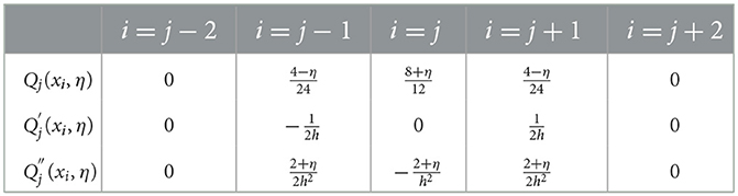
Table 1. Values of at knots.
Now, suppose that the approximate solution to the exact solution u(x, ti+1) at (i + 1)th time level given by
where δj are the parameters to be determined from the application of the collocation method, initial and boundary conditions. Using Table 1, evaluation of Eq. (16) and its first and second derivatives at knots xj yield
Using Eq. (17) at xj in Eq. (14), we get the system of N + 1 linear equations in N + 3 unknown as
This gives
where
σj = σ(xj, ε), aj = a(xj),
The two-variable method [38] for boundary value problem Eq. (14) with a(x) > 0 expresses the solution Ui+1(x) as
where is solution of the reduced problem
With the Taylor series expanding a(x) and di+1(x) about “1," and keeping the first term, we obtain
Eqs (19) and (21) at the nodal point xj are given by
and
In th limiting case as h → 0, we get
and
where ρ = h/ε. Similarly, computing the values of at xj−1, xj, xj+1 and adding in the proportion , respectively, and removing δj's using Eq. (23), we define
Since, and . We have
Thus, , which implies
For 0 ≤ j ≤ N, Eq. (19) is a system of (N + 1) linear equation in (N + 3) unknown δ−1, δ0, δ1, …, δN+1. Now, by applying boundary conditions, at i = 0 and i = N, for Eq. (19) and first equation of Eq. (17), we can eliminate δ−1 and δN+1. Therefore, we get
Finally, in (N + 1) unknowns δ0, δ1, …, δN, we find a system of (N + 1) equations with a matrix form as
where
As h → 0, R is diagonally dominant tridiagonal matrix, non-singular. Therefore, we can compute the values of δj's, then substituted in Eq. (16), to obtain the approximate solution to Eq. (14).
In this section, we establish the parameter-uniform convergence of the extended cubic B-spline collocation method. The following lemma will be used in the convergence analysis.
Lemma 4.1. The extended cubic B-spline set Λ = {Q−1, Q0, Q1, …, QN+1} defined in Eq. (15), satisfy the inequality
Proof. We know that
Let x = xi be a nodal point. Then, by the definition of Qj(x, η), we have
Now, for xj−1 < x < xj, from Table 1, we get
Thus,
Since, , which completes the proof. □
We will use the following error bound lemma for spline interpolation by Hall [39]. For π : a = x0 < x1 <, …, < xN = b, let , and . For simplicity, we write and
Lemma 4.2 ([39]). Let Y be the cubic spline associate with and the partitioning π. Then,
where
Since the mesh we have used is uniform, .
Theorem 4.1. Let S(x, η) be the collocation approximation from the space of cubic spline to the solution of ordinary differential equation. If , the parameter uniform error is given by
where h is sufficiently small and C is a positive constant independent of ε and N.
Proof. Let Ys(x) be unique spline interpolation from to the solution for boundary value problem Eq. (14) given by
If , then , and so using Lemma 4.2, we have
where λr's are independent of h and N. From the estimate Eq. (30), we obtain
Now, from Lemma (3.4), estimate Eq. (25) and using the argument that since ε≪1 and as ε → 0,∀x ∈ Ωx, we easily obtain
Let with boundary conditions Ys(0) = ψ0(ti+1), Ys(1) = ψ1(ti+1) leads to . Then, it follows with Eq. (28) that
where
It is obvious from inequality Eq. (31) that
In Eq. 19, implies . Therefore for η > −2 and sufficiently small values of h, matrix R is strictly diagonally dominant, thus non singular. So by the estimate given [40], we get
Combining of Eq. (32)–Eq. (34) gives
Using Eq. (26) and Eq. (27), we have
Therefore,
We define . Then,
This proves that the proposed finite difference scheme is unconditionally stable. The above inequality Eq. (36) together with Lemma 4.1 enables us to estimate |S(x)−Ys(x)|; hence, . We have
This gives . Therefore, using the triangular inequality, we obtain
hence the result. □
Theorem 4.2. Let u(x, t) be the solution of problem Eq. (1) and S(x, ti+1) be the collocation approximation from the space to the solution u(x, ti+1) at the (i + 1)th time level of the fully discretized scheme after the temporal discretization. If , the uniform error estimate is given by
Proof. The proof is the consequence of Lemma 3.3 and Theorem 4.1. □
In this section, we will see the applicability of the proposed method by considering two test problems. For each η = −1 value in the range [−8, 1], the computation was carried out to find the most valuable free parameter, which will give a minimum error. The least absolute errors were found for η = −1. For the remainder of the calculation, we have set up η = −1.
Example 5.1 ([41]). Consider the following test problem
We employ the following double mesh principle to determine the absolute error in the solution because the test problem's exact solution is unknown. For each ε, the maximum point wise error is given as
where SN, M and S2N, 2M are the computed solutions obtained on two different meshes DN, M and D2N, 2M respectively. D2N, 2M obtained from DN, M by the interpolation technique. The corresponding order of convergence is computed as
The ε-uniform point wise error EN, M is estimated as
and the ε-uniform order of convergence is calculated as
Example 5.2. Consider the following problem
We choose the initial data ψb(x, t) and the source function f(x, t) to fit with the exact solution
where p1 = exp(−1/ε) and p2 = 1−p1.
As we know the exact solution, we compute the point-wise error as
where and denote the exact and numerical solution obtained on DN, M. The corresponding computed order of convergence is calculated as
The ε- uniform point wise error and the corresponding order of convergence are calculated as
The numerical solution profiles for Example 5.1 and Example 5.2 at N = 64 and different values ε are graphically represented in Figures 1, 2, respectively. These figures shows the existence of boundary layer at x = 1, and it is clearly observed that width of the boundary layer decreases as perturbation parameter ε decreases, which is the effect of ε. Figures 3, 4 provide the numerical solution for test problem Example 5.1 and Example 5.2 for different values of t for fixed value of perturbation parameter ε at η = −1, where N = 64. Figure 5 provides the log-log plot of maximum absolute errors for Example 5.1 and Example 5.2. Figure 6 represents the graphs of the solution for various values of ε. Since the plots follow a straight line, this shows us that the maximum absolute point-wise error changes as a constant power of mesh parameter N. In addition, the negative slope of the lines states that the maximum absolute error decreases as the number of mesh points increases. In these figures, the plots are parallel, which shows the parameter-uniform convergence of the scheme. The maximum point wise error , ε-uniform errors , rate of convergence , and ε-uniform rate of convergence for Example 5.1 and Example 5.2 are presented in Tables 2, 3, respectively, at η = −1. The numerical results presented in Tables 2, 3 show that the proposed method is ε-uniformly convergent as for fixed value of ε. When N and M are increases, the maximum point wise error and the maximum nodal errors decreases. We see that the maximum point wise error and the rate of convergence stabilize as ε → 0 for each N and M. A comparison of maximum point wise error for 5.1 calculated by the proposed method at η = −1 and for in Kumar [8] is presented in Table 4. Computational results in Table 4 shows the proposed method provide more accurate solutions than in Kumar [8]. Furthermore, we note that all computations have been performed using MATLAB® R2022b software package (The Mathworks, Inc.), on a 64 bit Windows 11 hp CPU PC machine, with Intel(R) Core(TM) i3-3110M processor running at 2.40 GHz and 4.00 Gb RAM.
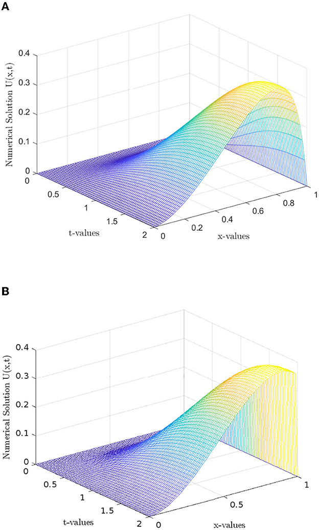
Figure 1. Numerical solution profile for Example 5.1, with N = 64, M = 80. (A) ε = 2−4. (B) ε = 2−15.
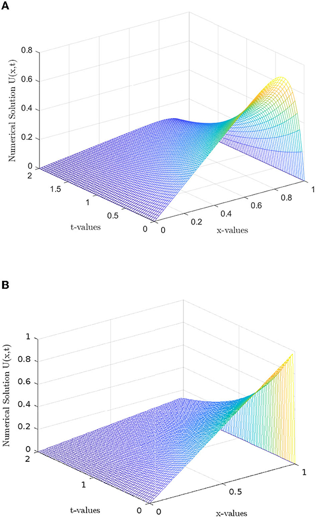
Figure 2. Numerical solution profile for Example 5.2, with N = M = 64. (A) ε = 2−4. (B) ε = 2−15.
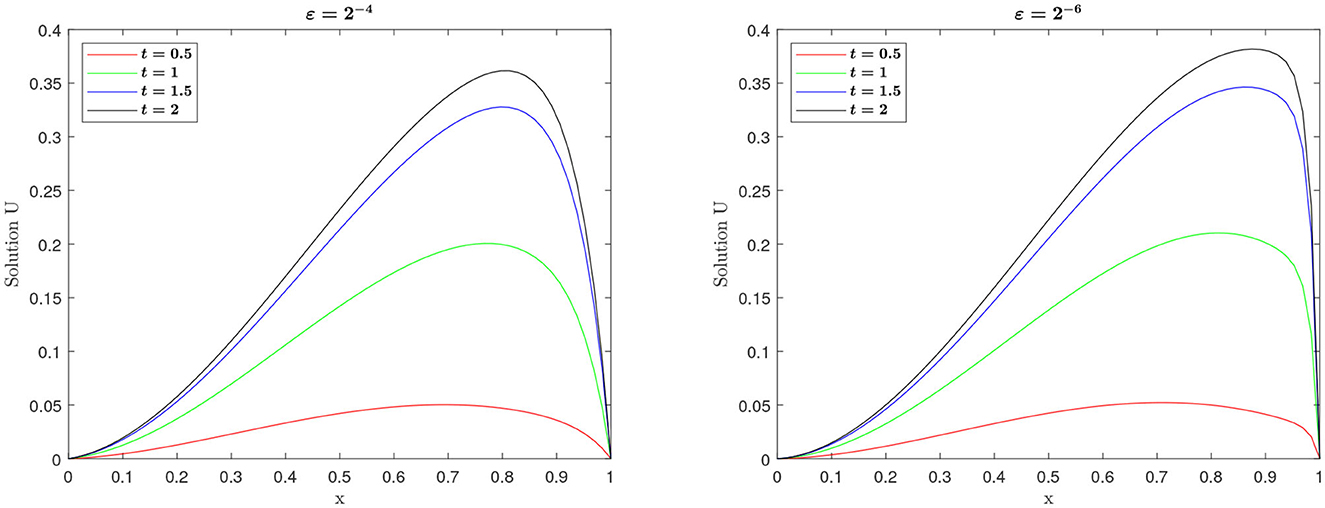
Figure 3. Numerical solution of Example 5.1 for different values of ε and t with N = 64 and M = 80.
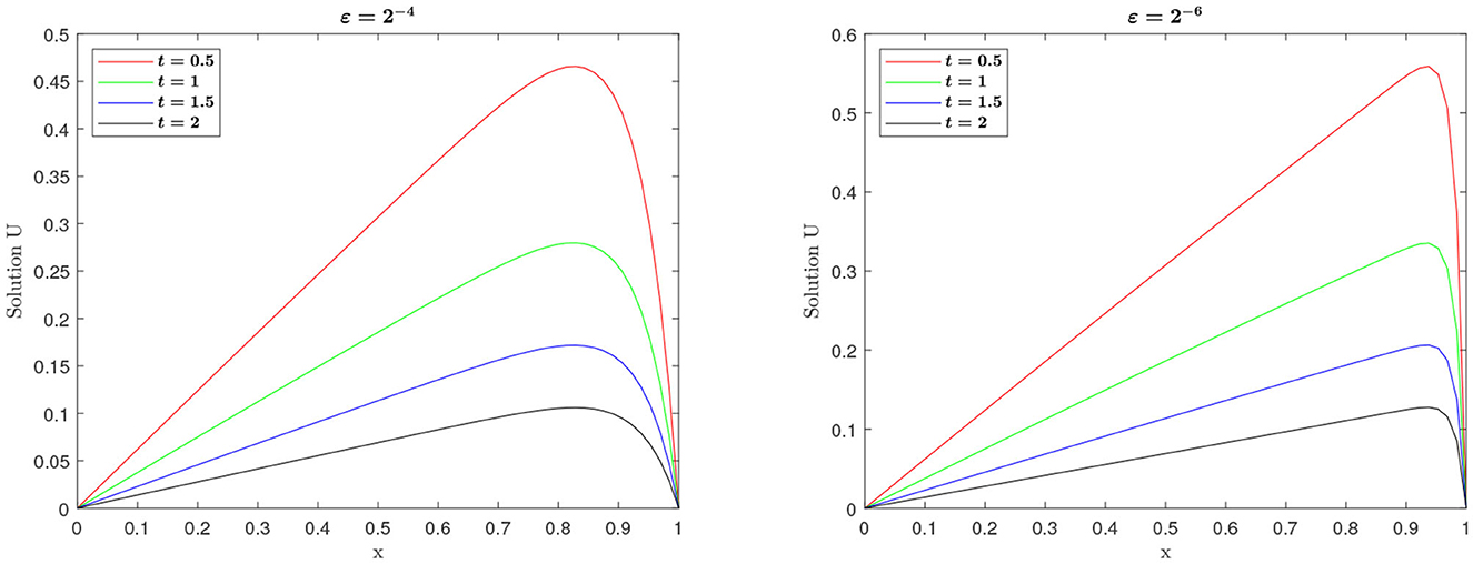
Figure 4. Numerical solution of Example 5.2 for different values of ε and t with N = M = 64.
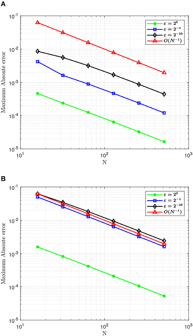
Figure 5. Log-log plot of maximum point wise error (A) for Example 5.1 and (B) for Example 5.2.
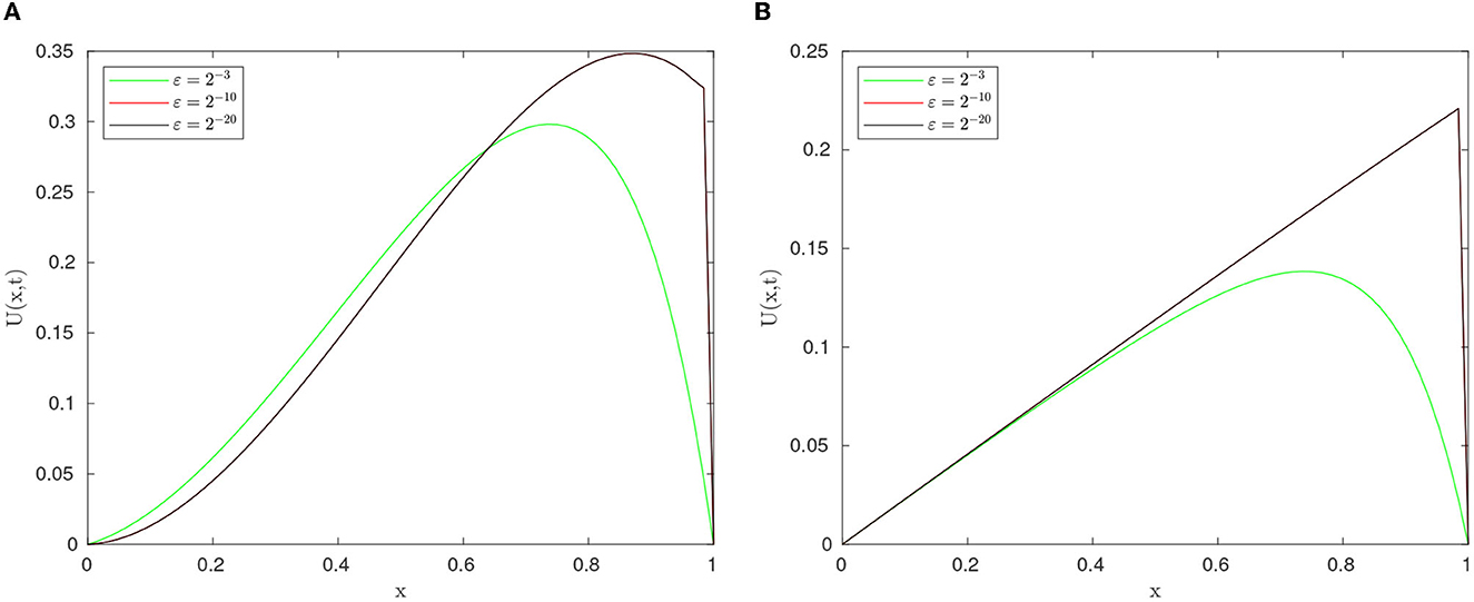
Figure 6. Effect of ε on the solution behavior at T = 1.5. (A) Example 5.1. (B) Example 5.2.
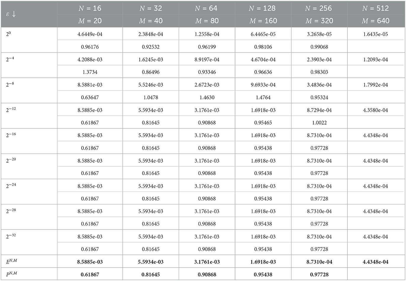
Table 2. Values of and PN, M for Example 5.1.
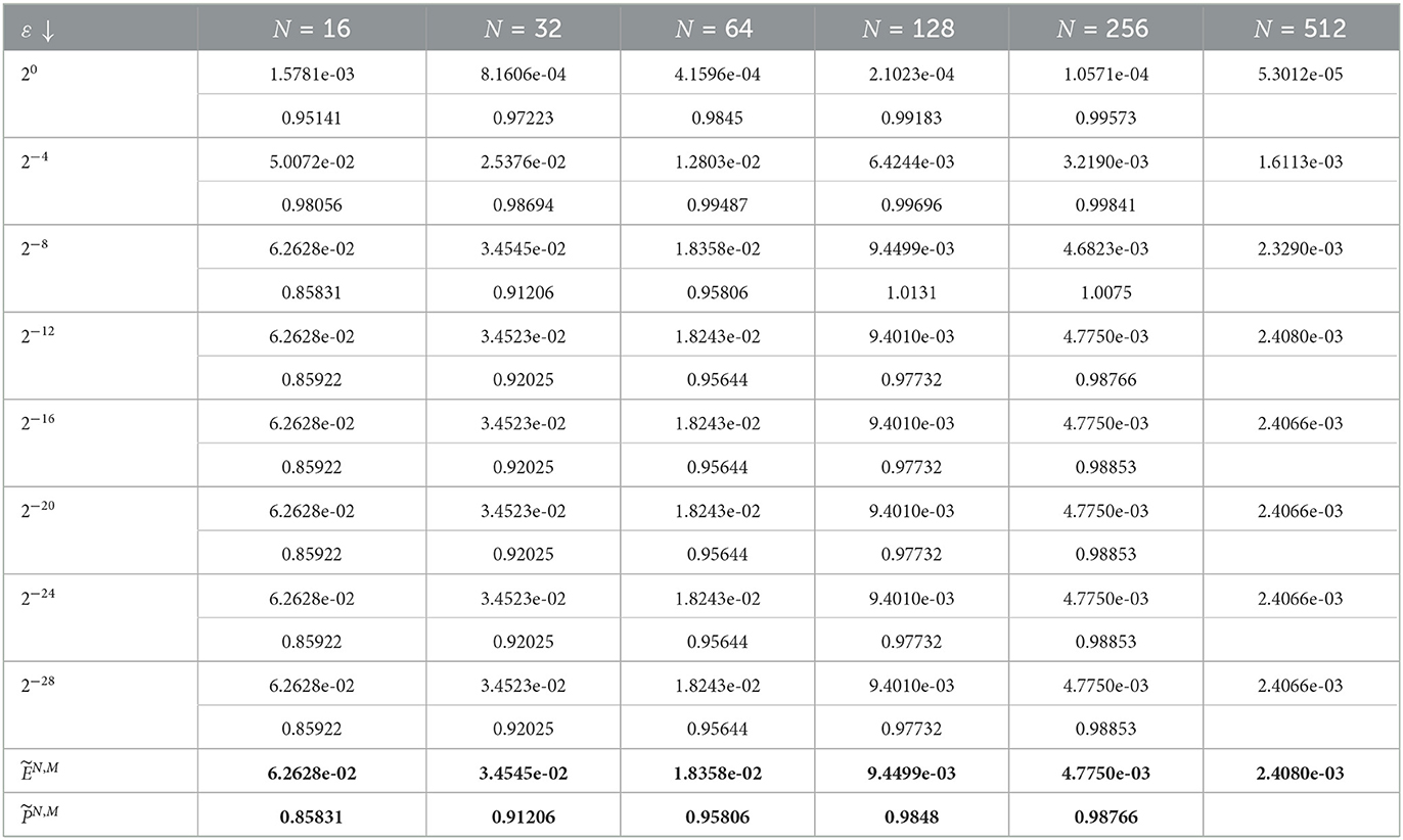
Table 3. and for Example 5.2.
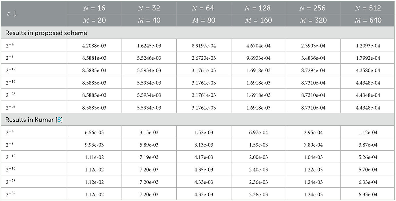
Table 4. Comparison of the maximum point-wise error for Example 5.1.
In this study, we provided a parameter uniform numerical scheme is developed to solve singularly perturbed parabolic convection-diffusion initial boundary value problems with large delay. The method is based on the implicit Euler method for temporal discretization and extended cubic B-spline collocation method with a blending function of degree four for spatial discretization using artificial viscosity both on the uniform mesh. The theoretical results which show the parameter-uniform convergence of the method are established and the proposed method is shown order . The scheme is also unconditionally stable. The appropriate choice of the free parameter η minimizes the error. To validate the theoretical results two test examples are presented. Graphical and tabular representations of the solutions and accuracy of the examples' results are provided. The numerical results obtained by the proposed method are compared with the numerical results in some existing literature.
As future directions of this study, we extend the proposed scheme for solving non-linear and higher dimensional singularly perturbed delay partial differential equations with Dirichlet boundary conditions.
The original contributions presented in the study are included in the article/supplementary material, further inquiries can be directed to the corresponding author.
ZH: Conceptualization, Formal analysis, Investigation, Methodology, Resources, Software, Writing—original draft, Writing—review and editing. GD: Conceptualization, Formal analysis, Investigation, Methodology, Resources, Software, Supervision, Writing—original draft, Writing—review and editing. All authors contributed to the article and approved the submitted version.
The authors kindly thank the editor for handling the manuscript carefully and referees for their valuable contributions in modifying the original version of the manuscript.
The authors declare that the research was conducted in the absence of any commercial or financial relationships that could be construed as a potential conflict of interest.
All claims expressed in this article are solely those of the authors and do not necessarily represent those of their affiliated organizations, or those of the publisher, the editors and the reviewers. Any product that may be evaluated in this article, or claim that may be made by its manufacturer, is not guaranteed or endorsed by the publisher.
1. Cooke K, Van den Driessche P, Zou X. Interaction of maturation delay and nonlinear birth in population and epidemic models. J Math Biol. (1999) 39:332–52. doi: 10.1007/s002850050194
2. Wang XT. Numerical solution of delay systems containing inverse time by hybrid functions. Appl Math Comput. (2006) 173:535–46. doi: 10.1016/j.amc.2005.04.056
3. Zhao T. Global periodic-solutions for a differential delay system modeling a microbial population in the chemostat. J Math Anal Appl. (1995) 193:329–52. doi: 10.1006/jmaa.1995.1239
4. Smolen P, Baxter DA, Byrne JH. A reduced model clarifies the role of feedback loops and time delays in the Drosophila circadian oscillator. Biophys J. (2002) 83:2349–59. doi: 10.1016/S0006-3495(02)75249-1
5. Vielle B, Chauvet G. Delay equation analysis of human respiratory stability. Math Biosci. (1998) 152:105–22. doi: 10.1016/S0025-5564(98)10028-7
6. Villasana M, Radunskaya A. A delay differential equation model for tumor growth. J Math Biol. (2003) 47:270–94. doi: 10.1007/s00285-003-0211-0
7. Wang PKC. Asymptotic stability of a time-delayed diffusion system. J Appl Mech. (1963) 30:500–4. doi: 10.1115/1.3636609
8. Kumar D. A parameter-uniform scheme for the parabolic singularly perturbed problem with a delay in time. Numer Methods Partial Differ Equ. (2021) 37:626–42. doi: 10.1002/num.22544
9. Wu J. Theory and Applications of Partial Functional Differential Equations, Vol 119. New York, NY: Springer Science & Business Media (1996). doi: 10.1007/978-1-4612-4050-1
10. Kuang Y. Delay Differential Equations: with Applications in Population Dynamics. Cambridge, MA: Academic press (1993).
11. Das A, Natesan S. Uniformly convergent hybrid numerical scheme for singularly perturbed delay parabolic convection-diffusion problems on Shishkin mesh. Appl Math Comput. (2015) 271:168–86. doi: 10.1016/j.amc.2015.08.137
12. Negero N, Duressa G. An efficient numerical approach for singularly perturbed parabolic convection-diffusion problems with large time-lag. J Math Model. (2022) 10:173–110. doi: 10.1016/j.rinam.2022.100338
13. Negero NT, Duressa GF. A method of line with improved accuracy for singularly perturbed parabolic convection-diffusion problems with large temporal lag. Results Appl Math. (2021) 11:100174. doi: 10.1016/j.rinam.2021.100174
14. Woldaregay MM, Aniley WT, Duressa GF. Novel numerical scheme for singularly perturbed time delay convection-diffusion equation. Adv Math Phys. (2021) 2021:1–13. doi: 10.1155/2021/6641236
15. Kumar K, Podila PC, Das P, Ramos H. A graded mesh refinement approach for boundary layer originated singularly perturbed time-delayed parabolic convection diffusion problems. Math Methods Appl Sci. (2021) 44:12332–50. doi: 10.1002/mma.7358
16. Abdelhakem M, Youssri Y. Two spectral Legendre's derivative algorithms for Lane-Emden, Bratu equations, and singular perturbed problems. Appl Numer Math. (2021) 169:243–55. doi: 10.1016/j.apnum.2021.07.006
17. Abd-Elhameed W, Youssri Y, Doha E. A novel operational matrix method based on shifted Legendre polynomials for solving second-order boundary value problems involving singular, singularly perturbed and Bratu-type equations. Math Sci. (2015) 9:93–102. doi: 10.1007/s40096-015-0155-8
18. Salama A, Al-Amery D. A higher order uniformly convergent method for singularly perturbed delay parabolic partial differential equations. Int J Comput Math. (2017) 94:2520–46. doi: 10.1080/00207160.2017.1284317
19. Gowrisankar S, Natesan S. ε-Uniformly convergent numerical scheme for singularly perturbed delay parabolic partial differential equations. Int J Comput Math. (2017) 94:902–21. doi: 10.1080/00207160.2016.1154948
20. Babu G, Bansal K. A high order robust numerical scheme for singularly perturbed delay parabolic convection diffusion problems. J Appl Math Comput. (2022) 68:363–89. doi: 10.1007/s12190-021-01512-1
21. Govindarao L, Mohapatra J. A second order numerical method for singularly perturbed delay parabolic partial differential equation. Eng Comput. (2018) 36:420–44. doi: 10.1108/EC-08-2018-0337
22. Podila PC, Kumar K. A new stable finite difference scheme and its convergence for time-delayed singularly perturbed parabolic PDEs. Comput Appl Math. (2020) 39:1–16. doi: 10.1007/s40314-020-01170-2
23. Hailu WS, Duressa GF. Parameter-uniform cubic spline method for singularly perturbed parabolic differential equation with large negative shift and integral boundary condition. Res Math. (2022) 9:2151080. doi: 10.1080/27684830.2022.2151080
24. Hassen ZI, Duressa GF. New approach of convergent numerical method for singularly perturbed delay parabolic convection-diffusion problems. Res Math. (2023) 10:2225267. doi: 10.1080/27684830.2023.2225267
25. Daba IT, Duressa GF. Extended cubic B-spline collocation method for singularly perturbed parabolic differential-difference equation arising in computational neuroscience. Int J Numer Method Biomed Eng. (2021) 37:e3418. doi: 10.1002/cnm.3418
26. Daba IT, Duressa GF. Collocation method using artificial viscosity for time dependent singularly perturbed differential-difference equations. Math Comput Simul. (2022) 192:201–20. doi: 10.1016/j.matcom.2021.09.005
27. Kumar D, Kadalbajoo MK. A parameter-uniform numerical method for time-dependent singularly perturbed differential-difference equations. Appl Math Model. (2011) 35:2805–19. doi: 10.1016/j.apm.2010.11.074
28. Negero NT, Duressa GF. Uniform convergent solution of singularly perturbed parabolic differential equations with general temporal-lag. Iran J Sci Technol Trans A Sci. (2022) 46:507–24. doi: 10.1007/s40995-021-01258-2
29. Kumar D, Kumari P. A parameter-uniform scheme for singularly perturbed partial differential equations with a time lag. Numer Methods Partial Differ Equ. (2020) 36:868–86. doi: 10.1002/num.22455
30. Stynes M, Stynes D. Convection-diffusion Problems: An Introduction to their Analysis and Numerical Solution, Vol 196. Washington, DC: American Mathematical Society; Atlantic Association for Research in the Mathematical Sciences (2018). doi: 10.1090/gsm/196
31. Mbroh NA, Noutchie SCO, Massoukou RYM. A robust method of lines solution for singularly perturbed delay parabolic problem. Alex Eng J. (2020) 59:2543–54. doi: 10.1016/j.aej.2020.03.042
32. Rothe E. Zweidimensionale parabolische randwertaufgaben als grenzfall eindimensionaler randwertaufgaben. Math Ann. (1930) 102:650–70. doi: 10.1007/BF01782368
33. Kadalbajoo MK, Gupta V, Awasthi A. A uniformly convergent B-spline collocation method on a nonuniform mesh for singularly perturbed one-dimensional time-dependent linear convection-diffusion problem. J Comput Appl Math. (2008) 220:271–89. doi: 10.1016/j.cam.2007.08.016
34. Kellogg RB, Tsan A. Analysis of some difference approximations for a singular perturbation problem without turning points. Math Comput. (1978) 32:1025–39. doi: 10.1090/S0025-5718-1978-0483484-9
35. Clavero C, Jorge J, Lisbona F. A uniformly convergent scheme on a nonuniform mesh for convection-diffusion parabolic problems. J Comput Appl Math. (2003) 154:415–29. doi: 10.1016/S0377-0427(02)00861-0
36. Dağ İ, Irk D, Sarı M. The extended cubic B-spline algorithm for a modified regularized long wave equation. Chin Phys B. (2013) 22:040207. doi: 10.1088/1674-1056/22/4/040207
37. Gang X, Guo-Zhao W. Extended cubic uniform B-spline and α-B-spline. Acta Autom Sin. (2008) 34:980–4. doi: 10.1016/S1874-1029(08)60047-6
38. O'Malley RE. Singular Perturbation Methods for Ordinary Differential Equations, Vol 89. New York, NY: Springer (1991). doi: 10.1007/978-1-4612-0977-5
39. Hall C. On error bounds for spline interpolation. J Approx Theory. (1968) 1:209–18. doi: 10.1016/0021-9045(68)90025-7
40. Varah JM. A lower bound for the smallest singular value of a matrix. Linear Algebra Appl. (1975) 11:3–5. doi: 10.1016/0024-3795(75)90112-3
Keywords: singularly perturbed delay differential equations, extended cubic B-spline collocation scheme, implicit Euler method, artificial viscosity, parabolic convection-diffusion, blending function
Citation: Hassen ZI and Duressa GF (2023) Parameter-uniformly convergent numerical scheme for singularly perturbed delay parabolic differential equation via extended B-spline collocation. Front. Appl. Math. Stat. 9:1255672. doi: 10.3389/fams.2023.1255672
Received: 09 July 2023; Accepted: 15 August 2023;
Published: 07 September 2023.
Edited by:
Vikas Gupta, LNM Institute of Information Technology, IndiaReviewed by:
Vivek Sangwan, Thapar Institute of Engineering and Technology, IndiaCopyright © 2023 Hassen and Duressa. This is an open-access article distributed under the terms of the Creative Commons Attribution License (CC BY). The use, distribution or reproduction in other forums is permitted, provided the original author(s) and the copyright owner(s) are credited and that the original publication in this journal is cited, in accordance with accepted academic practice. No use, distribution or reproduction is permitted which does not comply with these terms.
*Correspondence: Zerihun Ibrahim Hassen, emVyaWh1bmlicmFoaW1AZ21haWwuY29t
Disclaimer: All claims expressed in this article are solely those of the authors and do not necessarily represent those of their affiliated organizations, or those of the publisher, the editors and the reviewers. Any product that may be evaluated in this article or claim that may be made by its manufacturer is not guaranteed or endorsed by the publisher.
Research integrity at Frontiers
Learn more about the work of our research integrity team to safeguard the quality of each article we publish.