 Fekadu Mosisa Legesse
 Koya Purnachandra Rao
 Temesgen Duressa Keno
95% of researchers rate our articles as excellent or good
Learn more about the work of our research integrity team to safeguard the quality of each article we publish.
Find out more
ORIGINAL RESEARCH article
Front. Appl. Math. Stat. , 31 August 2023
Sec. Mathematical Biology
Volume 9 - 2023 | https://doi.org/10.3389/fams.2023.1224891
This article is part of the Research Topic Justified Modeling Frameworks and Novel Interpretations of Ecological and Epidemiological Systems View all 11 articles
The global impact of exclusive versus inclusive nursing on particular baby mortalities and morbidities from conception to 6 months is examined in this study. Exclusive breastfeeding practices are more crucial and effective in preventing illness outbreaks when there is no access to appropriate medications or vaccinations. Additionally, this study takes optimal control theory into account, applying it to a system of differential equations that uses Pontryagin's Maximum Principle to describe a bimodal pneumonia transmission behavior in a vulnerable compartment. The proposed pneumonia transmission model was then updated to include two control variables. These include preventing illness exposure in susceptible children through various preventative measures and treating infected children through antibiotics, hospital care, and other treatments. If the threshold number (ℜ0) is less than one, then treatment and prevention rates are increased, and the disease will be wiped out of the population. However, when (ℜ0) is greater than one, then the disease persists in the population, which indicates that prevention and treatment rates are low. To evaluate the cost-effectiveness of all potential control techniques and their combinations, the incremental cost-effectiveness ratio (ICER) was determined. The simulation results of the identified model show that the interventions of prevention and treatment scenarios were the most successful in eradicating the dynamics of the pneumonia disease's propagation during the epidemic, but they were ineffective from a cost-saving perspective. Therefore, limiting pneumonia transmission to prevention alone during an outbreak is the most economical course of action.
Infant (child) disability and death are the primary continuing public health issues worldwide. However, newborn (child) mortality and morbidity rates are greatly impacted by deaths caused by infectious illnesses. Infectious diseases can take 7 from 10 childhood deaths throughout the world. Pneumonia is one of the most common causes of death worldwide among acute respiratory infections, accounting for 30% of all child fatalities. Ninety-five percent of cases of pneumonia occur in developing countries. As a result, infectious illnesses are more likely to kill newborn babies in these countries [1, 2].
Among acute respiratory infection (ARI) diseases, pneumonia is the one that affects children's lungs. Approximately 740,180 children aged 05 years died because of pneumonia in 2019, which accounts for 14 and 22% of all deaths of children below 5 years and 1–5 year(s) old, respectively, and deaths are higher in Asia and Africa [3]. Hence, of infectious diseases, pneumonia causes the most children's deaths worldwide [4]. Pneumonia can be caused either by viruses, bacteria, or fungi; among these, bacterial pneumonia is the leading cause of death for children under 6 years of age. By immunizing against the disease, providing appropriate nutrition (EBF), and decreasing environmental variables, pneumonia can be avoided [5]. Additionally, using many control measures, such as prevention, treatment, and reducing indoor air pollution, can halt the spread of pneumonia. The following research has been carried out to address non-exclusive EBF or a lack of EBF, one of the main risk factors for infectious illnesses.
The first natural diet for infants is their mother's milk, which contains all the nutrients and energy required for a baby throughout the first 6 months of life [6]. According to WHO recommendations, newborns should receive only breast milk for the first 6 months of their lives. Thereafter, additional (complementary) foods are allowed for 18 months or more, followed by breastfeeding. Hence, infants (children) can achieve good growth and development [7]. Therefore, for children in the first months of life up to 6 months, any additional food or liquid (even water) is not permitted except vitamins, mineral supplements, and medicine[7, 8].
An intervention of double control has been offered to help eliminate the mortality and disability rates among children because of infectious diseases. Breastfeeding is one of the most popular and cost-effective strategies (interventions) for preventing pediatric pneumonia and all other causes of death [9–11]. Furthermore, the WHO, UNICEF, AAP, AAFP, and NNPE advocate starting breastfeeding promptly within the first hour after birth and continuing to exclusively breastfeed with human milk for the following 6 months to reduce the baby (child) death and disability rate. Continual breastfeeding with other appropriate foods will follow for the first 2 years of life to ensure that the children have healthy optimal growth and development [2].
Most of the studies assure that over two-thirds of the deaths occurring globally in the first year of life of children are often associated with a loss of exclusive breastfeeding or inappropriate feeding exercises [10]. Sub-optimal breastfeeding contributes to 18% of acute respiratory disease deaths among children under 5 years old in low-income countries [6].
Evidence suggests that if the EBF length is properly maintained, it can significantly increase immunity and lower the risk of death and disability from communicable and non-communicable diseases in both the early and advanced phases [12, 13]. EBF throughout the first 6 months of a baby's (or child's) life can typically lower the likelihood of developing any infectious diseases [14]. For the first 6 months of their lives, infants (children) who were nursed exclusively had a higher risk of contracting infectious diseases than those who were not [9, 15].
According to [10, 16], 1.24 million or 96% of child deaths occur during the first 6 months of life due to inappropriate EBF practices, and the mortality rate is higher in Africa and Asia. Additionally, poor breastfeeding results in more than 236,000 child deaths annually in a select few nations, including Nigeria, China, Mexico, Indonesia, and India [17]. Furthermore, in low- and middle-income nations, inadequate breastfeeding was found to be responsible for 18 and 30% of acute respiratory and diarrheal mortalities, respectively [18]. To reduce child mortality among children under the age of five, the WHO advises that an EBF of 90% is needed globally. Furthermore, the Sustainable Development Goals (SDGs) plan envisaged an increase in EBF of 50% by 2025 [19, 20]. According to the study by [12, 20], raising the EBF rate in middle-income and developing nations to an ideal level can reduce infant mortality among children under the age of five by 13 to 15%.
Mathematical models are frequently used to (i) analyse the dynamics of the spread of infectious diseases like cholera, bronchiolitis, pneumonia, and others; (ii) employ a variety of control methods to reduce or stop the spread of infectious diseases; and (iii) predict the effects of these diseases on people's lives, socio-economic systems, and national health programmes and policies. However, none of the aforementioned studies take into account a mathematical model method to illustrate the transmission behavior of infectious diseases, particularly pneumonia.
Several mathematical modeling studies have been conducted to estimate the potential burden of the endemic and the various control approaches for the endemic disease of pneumonia in children. Tilahun et al. [21] considered a non-linear deterministic model for the transmission of the pneumonia disease in a population of variable size, together with optimal control and cost-effectiveness measures. Agusto et al. [22] studied the advantage of isolation strategies and quarantine effectiveness measures against outbreaks of disease in the absence of appropriate medicines or vaccines.
Swai et al. [23] formulated an optimal control of pneumonia transmission in two strains by incorporating drug resistance. Additionally, how measures such as vaccination, public awareness campaigns, and therapy can reduce pneumonia transmission patterns should be considered. Tessema et al. [24] also developed a deterministic mathematical model of drug-resistant pneumonia with ideal preventive measures and cost-effectiveness evaluations. Based on the simulation values of optimal controls for the proposed model, they concluded that the combination of prevention, treatment, and screening of infectious persons is the most efficient and cost-effective way to remove pneumonia infections from the community. The diagnostic problem of distinguishing between bacterial and non-bacterial pneumonia is the main reason antibiotics are used to treat pneumonia in children. Consequently, Wu et al. [25] present causal Bayesian networks (BNs) in their model as useful tools for resolving this problem because they provide succinct maps of the probabilistic relationships between variables and produce results in a way that is understandable and justified by incorporating domain expert knowledge and numerical data.
Kotola and Mekonnen [26] created a deterministic model to demonstrate the efficacy of interventions for pneumonia and meningitis co-infection and provide a reasoned recommendation to public health officials, decision-makers in government policy, and programme implementers. Owing to their shared clinical characteristics and significant effects on human morbidity and mortality, pneumonia and tuberculosis are two of the most frequent airborne infections. Therefore, in a community of populations with both diseases, co-infection of the two diseases becomes inevitable. Owing to a lack of resources, the significant illness burden that these endemics together impose necessitates an efficient intervention to mitigate the impact. Thus, the authors in Gweryina et al. [27] use a pragmatic approach to create an SEIR model for the co-dynamics of tuberculosis and pneumonia. Using a variety of parameters, Naveed et al. [28] investigated the dynamics of delayed pneumonia-like infectious illnesses. Kassa et al. [29] and Rafiq et al. [30] offer a mathematical model of COVID-19 that includes bimodal virus transmission in a susceptible compartment.
Until now, only Legesse et al. [31] formulated a S1S2CIR deterministic mathematical model by grouping susceptible children as inclusively and exclusively breastfeed children and verify that inclusive breastfeeding children are more exposed to pneumonia than those children breastfeed exclusively. However, they did not take into account optimal control analysis in their research. Furthermore, no research has been carried out so far to assess the impact of EBF practice on child mortality rates and the efficacy of EBF practice in lowering pediatric mortality due to infectious disease (pneumonia). With this as a backdrop, the study's objective is to apply mathematical models with optimal control and accessible methods to treat pneumonia in infants between the ages of 0 and 6 months who do not participate in EBF. By increasing the prevalence of EBF and stepping up efforts to reduce non-exclusive breastfeeding, the findings of this study will help in making decisions that will reduce child mortality and impairment from pneumonia.
The article is organized as follows. The proposed model is formulated in the Construction of a Bimodal Pneumonia Model section and its analysis is presented in the Analyzing the Model Qualitatively section. Stability analysis of the equilibria is then discussed in the Equilibrium Point Stability section. Extension of the proposed model into optimal control is presented in The Proposed Model Under Optimal Control section. Numerical simulations are performed to support the analytical results discussed in the Analyzing the Model Qualitatively section and are presented in the Results and Discussion. Cost-effective analysis is performed in the subsequent section followed, finally, by the Conclusion.
In this model, the overall population size N(t) is divided into five mutually exclusive compartments based on the disease condition of the population as a whole. Furthermore, the total population size N(t) at any given time t is given by:
At any time instant t ∈ [0, ∞), the real valued differentiable state variables SI(t),SE(t),E(t),I(t), and R(t) represent the number of susceptible children that are not exclusively breastfed, susceptible children that are exclusively breastfed, children exposed to the disease, children that are seriously infected, and children who have obtained temporary immunity from pneumonia, respectively. This research assumes that the two susceptible classes SI(t) and SE(t) are enlisted into the population at rates of Λ1 and Λ2, respectively. They acquire pneumonia infection through effective contact with the infected humans I(t) or via inhalation of contaminated air droplets at a force of infection given by
, where i = 1, 2 and βj = kPj, where j = 1, 2.
Here βj = kPj for j = 1, 2 denotes the transmission rates. However, k stands for the number of contacts, and Pj is the probability of close contact rates between two susceptible humans with the infected individuals causing infection.
Humans exposed to pneumonia advance at a γ rate to the infected compartment I(t). The sub-populations are all reduced at the same time because a consistent natural mortality rate of μ is taken into account for each compartment. The parameters σ and α at the infected stage indicate the mortality rate from pneumonia disease, which only falls in the infected class, and the percentage of children who recover due to therapy or innate immunity, respectively. Those individuals that have recovered from pneumonia are assumed to have partial immunity and again become susceptible at a rate of δ. This study also assumes that a child who has obtained partial immunity does not again join exclusively breastfed children because as one individual is infected with infectious diseases they cannot regain their original immunity [31]. Using the parameter values, basic model assumptions, and state variables described above, we have generated a systematic diagram (Figure 1), and the corresponding model equation is given by Equation (2).
With the following initial conditions:
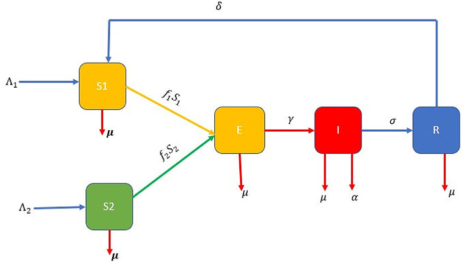
Figure 1. Model flow chart.
This subsection explains the qualitative behavior of the model being considered for the long run.
To ensure that the generated dynamical system's (2) positivity of solution is both epidemiologically meaningful and theoretically well-posed, we must show that all the state variables of the dynamical systems are non-negative.
Theorem 3.1. All the solutions of Equation (2) with the positive initial condition given on Equation (3) are non-negative.
Proof. From Equation (3), all the state variables are positive or zero at the initial time, then T > 0. To show the positivity of all the state variables select any equation of Equation (2), randomly let it be
where t′ ∈ [0, T] and each state variable are non-negative at t′.
Equation (4) is integrated with regard to time to produce
where . From Equation (4), we observe that SI(t) is non-negative for all t > 0. In a similar fashion, one can show SE(t) ≥ 0, E(t) ≥ 0, I(t) ≥ 0 and R(t) ≥ 0.
Theorem 3.2. The closed positive invariant set Ω is a biologically and mathematically well-posed region of the initial value problems defined on Equations (2), (3), where
Proof. For convenience, we let S1 = SI, S2 = SE, r1 = γ + μ, r2 = σ + α + μ, r3 = μ + δ throughout this study. Differentiating Equation (1) with respect to t gives
In the absence of infectious rate Equation (7) reduced to
Integrating both sides of Equation (8) with regard to t and taking the limit of Equation (8) as t → ∞, we obtain
Therefore, each solution of the initial value problems on Equations (2) and (3) remains in Equation (6) for all t > 0. This result can be summarized as lemma below.
Lemma 3.1. Ω is a positively invariant region for the Equation (2) with initial condition Equation (3) in .
Before calculating the expression for threshold quantity (ℜ0), determine pneumonia free of Equation (2). For this aim, equate the right hand side of Equation (2) to zero. After that, substitute in S1(t) = SI(0) > 0, SE(t) = SE(0) > 0, E(t) = E0 = I(t) = I0 and R(t) = R0 = 0. Thus,
Hence, E0 is the pneumonia free-equilibrium of Equation (2). By using DFE we can account the threshold number (ℜ0) following the work in Agusto [22], and we used the method of next generation matrix to obtain the required threshold number and from the transmission matrix
Where F1(t) = f1SI + f2SE and F2(t) = γE
and the transition matrix V is given by
where V1 = r1E and V2 = r2I.
Hence, using the next generation matrix calculated from Equations (12), (13) we get
Now, the governing eigenvalue of Equation (14) represents ℜ0 of Equation (2), which is given by
The threshold number (ℜ0) is a quantity that determines how pneumonia spreads within the population or fades out of the society. If ℜ0 < 1 then the disease will fade out of the community. This shows that more exclusivity in breastfeeding children is added to the susceptible class. Because exclusively breastfed individuals have high natural immunity, they are less exposed to the diseases. ℜ0 > 1 shows that there is a continuation of disease spread within the population.
In this part, we examine the condition known as EE of Equation (2). The fundamental motivation for this equilibrium is that it is utilized to estimate how long pneumonia will continue to affect the population. To identify the prerequisites for an equilibrium in which community pneumonia is endemic (that is, at least one of E* ≠ 0 or I* ≠ 0), denoted by . To find Ee, equate each equation in Equation (2) to zero and express each state variable in terms of the force of infection at the steady state ( where i=1,2), given by
Therefore, the existence of Ee in Equation (16) depends on ℜ0, meaning that Ee from Equation (2) exists if ℜ0 > 1.
The two equilibria of Equation (2) are shown in this subsection to have both local and global asymptotic stability. We employ the Jacobian matrices of system on Equation (2) at DFE and EE for local stability and the Lyapunov function for the global stability of both equilibria to confirm this stability.
Theorem 4.1. The disease free-equilibrium point (E0), of Equation (2) corresponding to the considered model is locally asymptotically stable if ℜ0 < 1 and not stable otherwise.
Proof. To prove this, first determine the Jacobian matrix evaluated at E0 becomes
The characteristic polynomial of Equation (17) becomes
The first three eigenvalues of Equation (18) are λ = −μ a double root, λ = −r3. All are negative, and we use the RouthHurwitz criterion to confirm the presence of the remaining eigenvalues in the manner described below:
As a result, the RouthHurwitz criteria's required condition is confirmed whenever ℜ0 < 1. Therefore, the DFE (E0) of Equation (2) is locally asymptotically stable (LAS) when ℜ0 < 1.
Theorem 4.2. The disease endemic equilibrium point (Ee), of Equation (2) is LAS in Ω if ℜ0 > 1 and unstable otherwise.
Proof. To prove the local stability of Ee, first determine the desired Jacobean matrix J(Ee) of system (2) at the endemic equilibrium, which is given as Equation (19)
The characteristics polynomial corresponding to Equation (19) is
The first three roots of Equation (20) are λ = −r1 < 0, λ = −r2 < 0, and λ = −r3 < 0 and the remaining roots can be calculated from
where
and are defined as the force of infection at the endemic equilibrium.
As has both roots with a negative real part (and the system with characteristic equation is stable) if and only if a1, a2 > 0, clearly a1, a2 > 0. Hence by RouthHurwitz criteria, for ℜ0 > 1, the endemic equilibrium (Ee) is LAS.
In this section, we use LaSalle's invariant principle to analyse the global stability of both equilibria of Equation (2) by creating suitable Lyapunov functions.
Theorem 4.3. If ℜ0 < 1, then the disease free-equilibrium (E0) of Equation (2) is GAS in Ω and unstable otherwise.
Proof. We first create a suitable Lyapunov function of the type
where ki, i = 1, 2 are positive real numbers to be chosen later. Upon differentiating Equation (21) along its trajectories with respect to t and simplifying, the result yields
Now, we choose k1 = γ and k2 = r1, and simplification of Equation (22) yields
Simplification and some rearrangement of Equation (23) will give:
Thus, whenever ℜ0 < 1. Additionally, if and only if E(t) = 0 and I(t) = 0. Hence, the largest compact invariant set is the singleton E0, which is the disease-free equilibrium. Therefore, using LaSalle's invariant principle [32], we conclude that the point E0 is globally asymptotically stable in Ω if ℜ0 < 1.
Theorem 4.4. The disease endemic equilibrium point (Ee) of Equation (2) is GAS in the invariant region stated in Theorem 3.2 as Ω if ℜ0 > 1.
Proof. To prove the global behavior of Ee, we systematically construct a Lyapunov function V of the form as Legesse et al. [31]
where xi represents the compartments in the model and i = 1,...5 and is the endemic equilibrium point. This is defined as
Then, after differentiating V with regard to time t, the following is obtained.
Next, substituting in Equation (26) using Equation (2) gives
We can put as where
Thus, if P < N, then . Hence, when ℜ0 > 1. Clearly, if and only if , and R = R*. Therefore, the largest compact positive invariant in set is the singleton Ee, which is a disease endemic equilibrium of Equation (2). Generally, by LaSalle's invariant principle, Ee is GAS in the biologically feasible region when ℜ0 > 1.
This section focuses on using optimum control techniques with the model under consideration from Equation (2). In a short amount of time, we were able to manage or reduce the diseases in the community with the use of these strategies. The pneumonia model is expanded to include the following two control variables, each of which is defined as follows:
u1: a campaign to prevent the spread of the disease among people who are vulnerable.
u2: by treating infectious diseases, a treatment effort is made to minimize infection or maximize recovery.
After incorporating u1 and u2 in Equation (2), we obtain the following optimal control model Equation (28).
The control set U is Lebesgue measurable and has the following definition in order to explore the optimal levels of the controls: U = {(u1(t), u2(t))}: {0 ≤ u1 < 1, 0 ≤ u2 < 1, 0 ≤ t ≤ T} where {0 ≤ u1 < 1, 0 ≤ u2 < 1, 0 ≤ t ≤ T} is the set of admissible controls. Our goal is to find a control u and SI, SE, E, I, and R that minimize the proposed objective function J given below, while maintaining the lowest cost of control implementation in Equation (2). The proposed objective functional J should follow the epidemic Equation (2), which is given by
subject to Equation (3), where b1 and b2 are the weight positive constants associated with the number of exposed children and infected children, respectively, while w1 and w2 are positive constants, present the relative cost weight, which is associated with control measures u1 and u2, respectively. We assume costs are non-linear in nature; hence, the control variables in J are in second degree polynomial form [21, 23]. The major thing that is required of us is to reduce the number of exposed and affected children while maintaining a low cost. Thus, we are going to find optimal controls , such that
where U = (u1, u2): each ui is measurable with 0 ≤ ui < 1 ,i = 1, 2 for t ∈ [0, tf].
Here, applying the principle of Pontryagin [34], Maximum Principle, we can drive the necessary conditions that the optimal control solution must satisfy [35]. Therefore, this principle converts the model Equations (28), (29) into a problem of minimizing a Hamiltonian, H, point-wise with respect to u1 and u2, and we obtained a Hamiltonian (H) defined as:
where
where
Hence the Hamiltonian becomes
where are the adjoint variable functions which are determined by using Pontryagin's maximal principle [34] and use Swai et al. [23] for verification of existence of the optimal control pairs.
Theorem 5.1. There exists adjoint variable λi, where i = 1, ..., 5 with transversality conditions λi(tf) = 0, i = 1, ..., 5 for an optimal control that minimizes J(u1, u2) such that:
where and λ(T) = 0 transidentality condition.
Now,
In a similar manner, we obtained the controls by solving the equation at , for i = 1, 2 in accordance with Pontryagin [34]'s methodology and obtained:
Similarly
From this
This implies that
The above equation in compact notation is
Considering the bounds of the control quintuple, we have
The optimality system is obtained from the state Equation (29) together with adjoint variables and the transversality condition in Theorem 5.1 by including the characterized control set and initial condition.
Therefore, using the optimality system 32, it is possible to calculate the optimal control. Consequently, the optimal problem is minimal at control and , as shown by the fact that the second derivatives of the Lagrangian with regard to u1 and u2, respectively, are positive.
To analyse the dynamics of pneumonia disease with or without control measures, numerical simulations are performed on the suggested model and optimality system using the parameter values indicated in Table 1. In addition, we assumed the initial population size to be SI(0) = 40; SE(0) = 100; E(0) = 50; I(0) = 15; and R(0) = 1 for the purpose of numerical simulation. The weight constant values are chosen as b1 = 3; b2 = 3; w1 = 0.05 and w2 = 0.03. First, we simulate the pneumonia model for the case R0 = 0.8513 < 1, which indicates that the pneumonia disease dies out from the society. As a result, the pneumonia model's solution trajectory moves toward a disease-free equilibrium point. The disease-free equilibrium point is demonstrated to be locally asymptotically stable as all the trajectories of the model converge to DFE, see Figure 2A. Next, we plotted the graphics for the case R0 = 1.4232 > 1, which implies that the disease is endemic. In this case, the solution curves are converging to the endemic equilibrium point, which verifies the linear stability of the EE point (see Figure 2B).
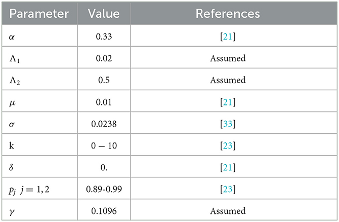
Table 1. Pneumonia model parameter values with their source.
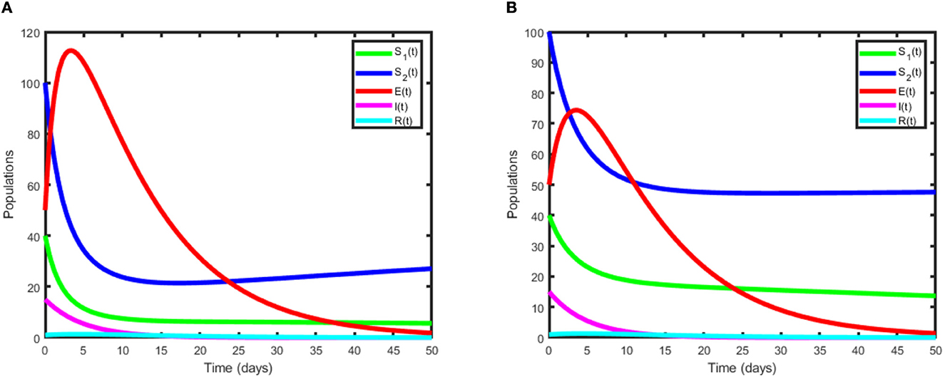
Figure 2. The pneumonia model's trajectory of solutions converges to (A) DFEP and (B) EEP.
Now, to extend the proposed model to optimal control, we focus on the parameter values and initial population, which give R0 = 1.4232 > 1 to analyze the model. In light of the fact that diseases are still prevalent in society, adding control factors to the mode is appropriate. Figures 3–6 demonstrate the impact of prevention and treatment on the dynamics of pneumonia.
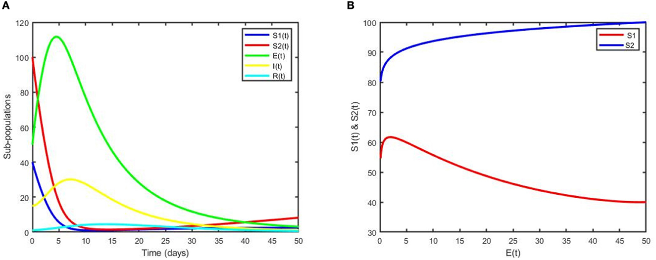
Figure 3. (A) Dynamics of sub-populations for the DFE point. (B) The phase portrait for SI(t) and SE(t) vs. E(t).
The plot in Figure 3A illustrates that subpopulations converge to the DFE point, which indicates that pneumonia has been eliminated from the community. Moreover, it can be observed that the two susceptible populations decrease while the exposed and infected children increase for a few years and decrease rapidly afterward to the DFE point. Figure 3B reveals that even if controls are applied, non-exclusively breastfed children are more exposed to pneumonia than exclusively breastfed children. In general, from Figures 2A, 3A, we can easily see the impact of control variables on the transmission dynamics of pneumonia.
We utilized the following scenarios to assess how each regulation would affect the dynamics of pneumonia spread:
(i) Optimal use of prevention (u1 only).
(ii) Optimal use of treatment (u2 only).
(iii) Optimal use of prevention (u1) and treatment (u2) intervention.
This scenario shows the use of only one control measure, prevention (u1), and the other controls were set to zero. As clearly observed from Figures 4A, B, with the optimal use of a prevention strategy, the two susceptible individuals increase due to the prevention strategy, and when we compare it with the case free of prevention, the number of susceptibilities of individuals to the diseases is less. Moreover, the number of total exposed humans decreases more with control than when there is no control, as depicted in Figure 4C. Since the number of infection averted human from pneumonia disease due to this strategy is less in number, hence additional intervention is required.
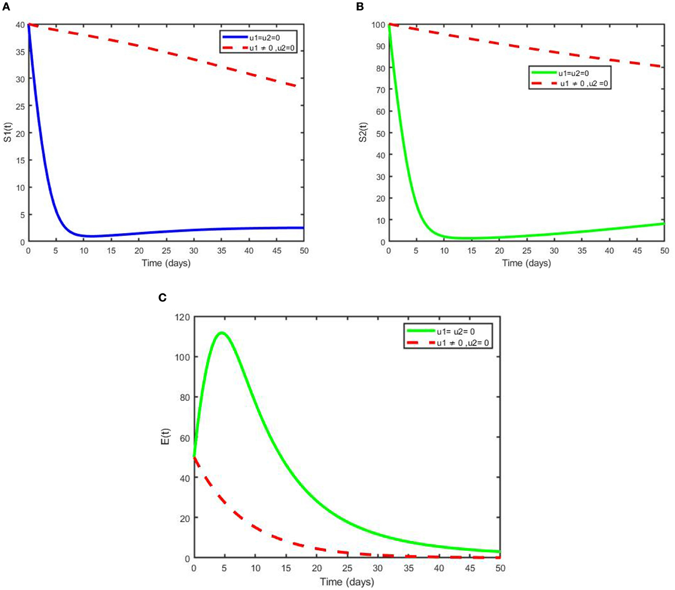
Figure 4. Simulation of the optimal model showing the effect of prevention on (A) not exclusively breastfeed individuals, (B) exclusively breastfeed individuals, and (C) exposed individuals.
Scenario B is shown in Figures 5A, B, which illustrate that treatment has a significant impact in reducing the number of children infected with pneumonia after 14 years. It can be noted that the number of infected individuals slightly decreases and becomes effective after some time; hence, more interventions are needed to eliminate the disease from the community.
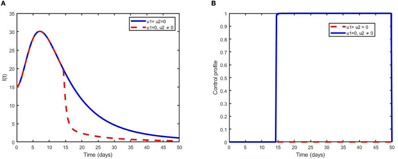
Figure 5. Simulations showing (A) the optimal use of treatment only (u2) and (B) its control profile.
This strategy demonstrates the effect of the optimal use of prevention for the exposed humans and treatment for the infectious humans to decrease the number of exposed and infected individuals in the society. Additionally, this intervention reduces the spread of pneumonia dynamics governed by model (2) in the population. The numbers of exposed individuals and infectious individuals decrease more rapidly when the two control scenarios are in use compared with when controls are not used or one control is used, as depicted in Figures 6A, B. Figure 6F reveals that the optimal use of prevention. u1(t) is maximum at 100% throughout the proposed days until reaching the final time that maximum prevention is applied to control pneumonia. Optimal use of treatment u2(t) is kept at the maximum level for 48 days before arriving at the minimum at the final intervention time. Figures 6C–E reveal, respectively, the size of SI, SE, and R increases compared with non-control and one control intervention. This confirms that a maximum number of children's pneumonia diseases are averted due to the intervention of the two controls.
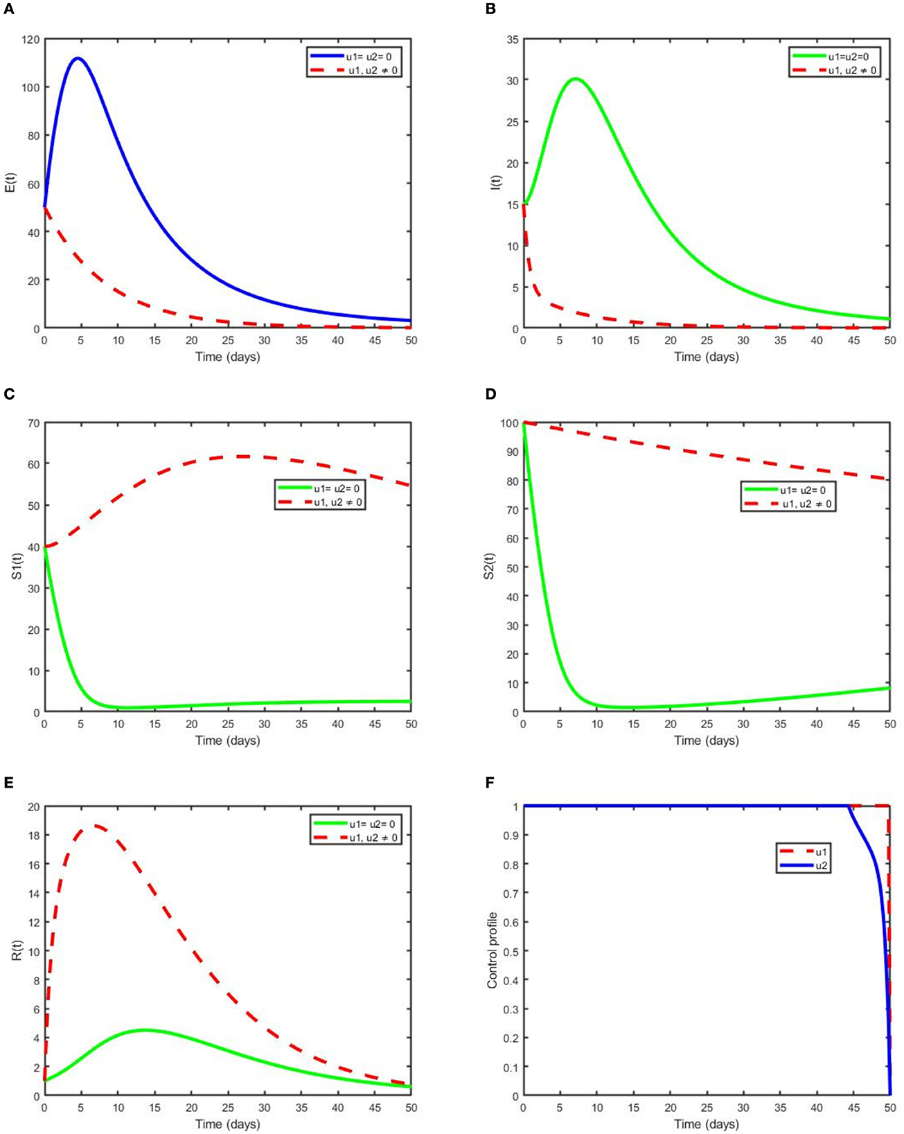
Figure 6. Simulations demonstrating optimal use of prevention (u1) and treatment (u2) on (A) E (B) I (C) SE (D) SI (E) R and (F) its control profile.
In this section, we present cost-effectiveness analysis, which is used to evaluate the benefits related to a health intervention(s) or strategy (strategies) (for instance treatment and prevention), to elaborate the strategy's costs [22]. The number of infections averted is given as the difference between total infectious individuals without control and total infectious individuals with control. Using the parameter values in Table 1 and initial conditions of state variables with the weight constant values chosen, the ICER is determined for each intervention labeled as prevention, treatment, and a combination of both. The prevention strategy includes vaccination (immunization), personal hygiene, avoiding exposure to people who are ill, covering a cough, and adequate nutrition (scenario A), while the treatment intervention involves antibiotics that stop the infection from progressing (these medicines are used to treat bacterial pneumonia), hospital treatment (allowed for more severe cases), rest, etc. (scenario B). The combination of prevention and treatment scenario C. This is obtained by balancing the change between the costs and health outcomes of these intervention strategies; usually obtained by using the incremental cost-effectiveness ratio (ICER), which is described as:
where the numerator of the ICER represents the difference in cost-benefit and the denominator measures the change in health benefit.
According to the simulation outcomes of the optimality system, the control scenarios are then ranked in ascending order of total number of infections averted, i.e., prevention of infections in susceptible children using vaccines, personal hygiene and others (strategy A), treatment of infected individuals with antibiotics (strategy B), and a combination of prevention and treatment (strategy C), as shown in Table 2.
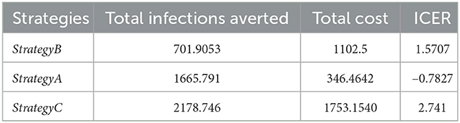
Table 2. Incremental cost-effectiveness ratio in increasing order of total infections averted.
The ICER is obtained through the following computation:
Now, comparing strategy A and B incrementally, the ICER for the two competing strategies is calculated as above and it shows that ICER (B) > ICER (A). From this, we can see that strategy A saves 0.7827 more than strategy B, and strategy B is a bit more expensive. Hence, we excluded strategy B from the set of competing strategies, and finally, we compared strategies A and C as depicted in Table 3. From ICER (A) and ICER (C) in Table 3 we can see that strategy C saves 2.741 than strategy A. Hence, we exclude strategy C, because it is a bit expensive. Therefore, we conclude that strategy A the cheapest of all compared strategies, that meant it is the most cost-effective for pneumonia disease control intervention strategies.
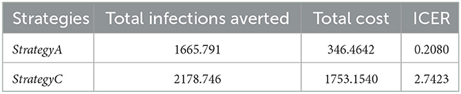
Table 3. Comparison between intervention strategies A and C.
This study is concerned with the mathematical analysis of a pneumonia transmission model with naturally acquired immunity in the presence of effective exclusively breastfed infants and a lack of naturally acquired immunity due to the loss of exclusively breastfed infants. This work also shows that if the threshold number is smaller than unity, then the pneumonia-free equilibrium point is both locally and globally asymptotically stable, which means pneumonia is wiped out of the community. If the threshold number is greater than unity, then an endemic equilibrium of the model occurs, which shows the persistence of the diseases in the population.
To control pneumonia spread dynamics in a population, multiple time-dependent control variables, including prevention using vaccines, personal hygiene, etc., treatment of infectious humans using antibiotics, hospital treatment, and rest are considered. An analysis of the optimal control model is carried out theoretically, and the model is simulated to determine the effects of combining the two control intervention strategies on the spread dynamics of pneumonia in the community. It is shown that the number of infected children is minimized through prevention and treatment intervention strategies. Throughout this work, based on the results in Table 3, we recommend the prevention of susceptible children from being exposed to the diseases using vaccination, public health education, etc., to reduce new exposed cases and the number of infected children due to pneumonia in our society with the least cost.
In general, we considered cleanliness as a method of preventing pneumonia in children under the age of five in the earlier studies on the dynamics of bimodal pneumonia [31]. However, in the present study, we considered the extension of the bimodal pneumonia model to optimal control using two time-dependent control measures, namely prevention and treatment. In addition, we analyzed the cost-effectiveness of intervention strategies. The result of the analysis reveals that prevention strategies are the most cost-effective way of eradicating pneumonia. Therefore, the present study is more effective and cost-effective in preventing pneumonia transmission than the previous study.
The original contributions presented in the study are included in the article/supplementary material, further inquiries can be directed to the corresponding author.
FL conceptualized, planned, and prepared the article as well as the figures. The final manuscript's review, modification, and literature search were all aided by the efforts of all writers. The article's submission was reviewed and approved by all authors.
The authors declare that the research was conducted in the absence of any commercial or financial relationships that could be construed as a potential conflict of interest.
All claims expressed in this article are solely those of the authors and do not necessarily represent those of their affiliated organizations, or those of the publisher, the editors and the reviewers. Any product that may be evaluated in this article, or claim that may be made by its manufacturer, is not guaranteed or endorsed by the publisher.
1. Elyas L, Mekasha A, Admasie A, Assefa E. Exclusive breastfeeding practice and associated factors among mothers attending private pediatric and child clinics, Addis Ababa, Ethiopia: a cross-sectional study. Int J Pediatr. (2017) 2017:8546192. doi: 10.1155/2017/8546192
2. Abdulla F, Hossain MM, Karimuzzaman M, Ali M, Rahman A. Likelihood of infectious diseases due to lack of exclusive breastfeeding among infants in Bangladesh. PLoS ONE. (2022) 17:e0263890. doi: 10.1371/journal.pone.0263890
3. Morty RE. World health day observances in November 2021: advocating for adult and pediatric pneumonia, preterm birth, and chronic obstructive pulmonary disease. Am J Physiol Lung Cell Mol Physiol. (2021) 321:L954L957. doi: 10.1152/ajplung.00423.2021
4. Otoo D, Opoku P, Charles S, Kingsley AP. Deterministic epidemic model for (SVCSyCAsyIR) pneumonia dynamics, with vaccination and temporal immunity. Infect Dis Model. (2020) 5:42–60. doi: 10.1016/j.idm.2019.11.001
5. Kizito M, Tumwiine J, A. mathematical model of treatment and vaccination interventions of pneumococcal pneumonia infection dynamics. J Appl Mathem. (2018) 2018:2539465. doi: 10.1155/2018/2539465
6. Alebel A, Tesma C, Temesgen B, Ferede A, Kibret GD. Exclusive breastfeeding practice in Ethiopia and its association with antenatal care and institutional delivery: a systematic review and meta-analysis. Int Breastfeed J. (2018) 13:1–12. doi: 10.1186/s13006-018-0173-x
7. Rajeshwari K, Bang A, Chaturvedi P, Kumar V, Yadav B, Bharadva K, et al. Infant and young child feeding guidelines: 2010. Indian Pediatr. (2010) 47:995–1004.
8. Arage G, Gedamu H. Exclusive breastfeeding practice and its associated factors among mothers of infants less than six months of age in Debre Tabor town, Northwest Ethiopia: a cross-sectional study. Adv Public Health. (2016) 2016:3426249. doi: 10.1155/2016/3426249
9. Turin CG, Ochoa TJ. The role of maternal breast milk in preventing infantile diarrhea in the developing world. Curr Trop Med Rep. (2014) 1:97–105. doi: 10.1007/s40475-014-0015-x
10. Tewabe T, Mandesh A, Gualu T, Alem G, Mekuria G, Zeleke H. Exclusive breastfeeding practice and associated factors among mothers in Motta town, East Gojjam zone, Amhara Regional State, Ethiopia, 2015: a cross-sectional study. Int Breastfeed J. (2016) 12:1–7. doi: 10.1186/s13006-017-0103-3
11. Mgongo M, Mosha MV, Uriyo JG, Msuya SE, Stray-Pedersen B. Prevalence and predictors of exclusive breastfeeding among women in Kilimanjaro region, Northern Tanzania: a population based cross-sectional study. Int Breastfeed J. (2013) 8:1–8. doi: 10.1186/1746-4358-8-12
12. Mogre V, Dery M, Gaa PK. Knowledge, attitudes and determinants of exclusive breastfeeding practice among Ghanaian rural lactating mothers. Int Breastfeed J. (2016) 11:1–8. doi: 10.1186/s13006-016-0071-z
13. Ajetunmobi OM, Whyte B, Chalmers J, Tappin DM, Wolfson L, Fleming M, et al. Breastfeeding is associated with reduced childhood hospitalization: evidence from a Scottish Birth Cohort (1997-2009). J Pediatr. (2015) 166:620–5. doi: 10.1016/j.jpeds.2014.11.013
14. Martin CR, Ling PR, Blackburn GL. Review of infant feeding: key features of breast milk and infant formula. Nutrients. (2016) 8:279. doi: 10.3390/nu8050279
15. Arifeen S, Black RE, Antelman G, Baqui A, Caulfield L, Becker S. Exclusive breastfeeding reduces acute respiratory infection and diarrhea deaths among infants in Dhaka slums. Pediatrics. (2001) 108:e67–e67. doi: 10.1542/peds.108.4.e67
16. Sefene A, Birhanu D, Awoke W, Taye T. Determinants of exclusive breastfeeding practice among mothers of children age less than 6 month in Bahir Dar city administration, Northwest Ethiopia; a community based cross-sectional survey. Sci J Clin Med. (2013) 2:153–9. doi: 10.11648/j.sjcm.20130206.12
17. Collective GB UNICEF. Nurturing the health and wealth of nations: the investment case for breastfeeding. Technical Report, World Health Organization. (2017).
18. Bhandari N, Chowdhury R. Infant and young child feeding. Proc Indian Nat Sci Acad. (2016) 82:1507–17. doi: 10.16943/ptinsa/2016/48883
19. Organization WH. Tracking universal health coverage: first global monitoring report. World Health Organization. (2015).
20. Sajjad S, Roshan R, Tanvir S. Impact of maternal education and source of knowledge on breast feeding practices in Rawalpindi city. MOJCRR. (2018) 1:212–42. doi: 10.15406/mojcrr.2018.01.00035
21. Tilahun GT, Makinde OD, Malonza D. Modelling and optimal control of pneumonia disease with cost-effective strategies. J Biol Dyn. (2017) 11:400–26. doi: 10.1080/17513758.2017.1337245
22. Agusto FB. Optimal isolation control strategies and cost-effectiveness analysis of a two-strain avian influenza model. Biosystems. (2013) 113:155–64. doi: 10.1016/j.biosystems.2013.06.004
23. Swai MC, Shaban N, Marijani T. Optimal control in two strain pneumonia transmission dynamics. J Appl Mathem. (2021) 2021:8835918. doi: 10.1155/2021/8835918
24. Tessema FS, Bole BK, Rao PK. Optimal control strategies and cost effectiveness analysis of Pneumonia disease with drug resistance. Int J Nonl Analy Appl. (2023) 14:903–17. doi: 10.22075/ijnaa.2022.26746.3402
25. Wu Y, Mascaro S, Bhuiyan M, Fathima P, Mace AO, Nicol MP, et al. Predicting the causative pathogen among children with pneumonia using a causal Bayesian network. PLoS Comput Biol. (2023) 19:e1010967. doi: 10.1371/journal.pcbi.1010967
26. Kotola BS, Mekonnen TT. Mathematical model analysis and numerical simulation for codynamics of meningitis and pneumonia infection with intervention. Sci Rep. (2022) 12:1–22. doi: 10.1038/s41598-022-06253-0
27. Gweryina RI, Madubueze CE, Bajiya VP, Esla FE. Modeling and analysis of tuberculosis and pneumonia co-infection dynamics with cost-effective strategies. Results Control Optimiz. (2023) 10:100210. doi: 10.1016/j.rico.2023.100210
28. Naveed M, Baleanu D, Raza A, Rafiq M, Soori AH, Mohsin M. Modeling the transmission dynamics of delayed pneumonia-like diseases with a sensitivity of parameters. Adv Differ Equat. (2021) 2021:1–19. doi: 10.1186/s13662-021-03618-z
29. Kassa SM, Njagarah JB, Terefe YA. Analysis of the mitigation strategies for COVID-19: from mathematical modelling perspective. Chaos, Solitons Fractals. (2020) 138:109968. doi: 10.1016/j.chaos.2020.109968
30. Rafiq M, Ali J, Riaz MB, Awrejcewicz J. Numerical analysis of a bi-modal COVID-19 sitr model. Alexandria Eng J. (2022) 61:227–35. doi: 10.1016/j.aej.2021.04.102
31. Legesse FM, Rao KP, Keno TD. Mathematical Modeling of a Bimodal Pneumonia Epidemic with Non-breastfeeding Class. Appl Math. (2023) 17:95–107. doi: 10.18576/amis/170111
32. Dano LB, Rao KP, Keno TD. Modeling the combined effect of hepatitis b infection and heavy alcohol consumption on the progression dynamics of liver cirrhosis. J Mathematics. (2022) 2022:6936396. doi: 10.1155/2022/6936396
33. Otieno O, Joseph M, John O. “Mathematical Model for Pneumonia Dynamics among Children,” in The 2012 southern Africa mathematical sciences association conference (SAMSA 2012). (2012).
Keywords: inclusive and exclusive, cost-effectiveness, pneumonia, optimal control, S1S2EIR model, ICER, breastfeeding
Citation: Legesse FM, Rao KP and Keno TD (2023) Cost effectiveness and optimal control analysis for bimodal pneumonia dynamics with the effect of children's breastfeeding. Front. Appl. Math. Stat. 9:1224891. doi: 10.3389/fams.2023.1224891
Received: 18 May 2023; Accepted: 02 August 2023;
Published: 31 August 2023.
Edited by:
Asep K. Supriatna, Padjadjaran University, IndonesiaReviewed by:
Arrival Rince Putri, Andalas University, IndonesiaCopyright © 2023 Legesse, Rao and Keno. This is an open-access article distributed under the terms of the Creative Commons Attribution License (CC BY). The use, distribution or reproduction in other forums is permitted, provided the original author(s) and the copyright owner(s) are credited and that the original publication in this journal is cited, in accordance with accepted academic practice. No use, distribution or reproduction is permitted which does not comply with these terms.
*Correspondence: Fekadu Mosisa Legesse, ZmVrYWR1bW9zaXNhMjJAZ21haWwuY29t
Disclaimer: All claims expressed in this article are solely those of the authors and do not necessarily represent those of their affiliated organizations, or those of the publisher, the editors and the reviewers. Any product that may be evaluated in this article or claim that may be made by its manufacturer is not guaranteed or endorsed by the publisher.
Research integrity at Frontiers
Learn more about the work of our research integrity team to safeguard the quality of each article we publish.