Modeling visceral leishmaniasis and tuberculosis co-infection dynamics

The co-infection of visceral leishmaniasis (VL) and tuberculosis (TB) patients pose a major public health challenge. In this study, we develop a mathematical model to study the transmission dynamics of VL and TB co-infection by first analyzing the VL and TB sub-models separately. The dynamics of these sub-models and the full co-infection model are determined based on the reproduction number. When the associated reproduction number (${\mathcal{R}}_1$) for the TB-only model and (${\mathcal{R}}_2$) for the VL-only are less than unity, the model exhibits backward bifurcation. If $max\left\{{\mathcal{R}}_1,{\mathcal{R}}_2\right\}={\mathcal{R}}_1$, then the TB-VL co-infection model exhibits backward bifurcation for values of ${\mathcal{R}}_1$. Furthermore, if $max\left\{{\mathcal{R}}_1,{\mathcal{R}}_2\right\}={\mathcal{R}}_2$, and by choosing the transmission probability, β_L as the bifurcation parameter, then the phenomenon of backward bifurcation occurs for values of ${\mathcal{R}}_2$. Consequently, the full model, whose associated reproduction number is ${\mathcal{R}}_0$, also exhibits backward bifurcation when ${\mathcal{R}}_0=1$. The equilibrium points and their stability for the models are determined and analyzed based on the magnitude of the respective reproduction numbers. Finally, some numerical simulations are presented to show the reliability of our theoretical results.

1. Introduction

Leishmaniasis is a neglected tropical disease (NTD) that is transmitted by infected sandflies and is caused by obligate intracellular protozoans of the genus Leishmania [1]. There are more than 20 Leishmania species with three main forms of the disease: cutaneous leishmaniasis, mucocutaneous leishmaniasis, and visceral leishmaniasis, also known as kala-azar. Cutaneous leishmaniasis (CL) is the most common form of leishmaniasis and causes skin lesions, mainly ulcers, on exposed parts of the body, leaving life-long scars and serious disability or stigma. Mucocutaneous leishmaniasis (MCL) is the most disabling form of the disease, and it affects mostly the mucous membranes of the nose and mouth. Visceral leishmaniasis (VL) is the most fatal disease, causing enlargement of the spleen and liver [2]. It may cause epidemic outbreaks with a high mortality rate. A varying proportion of visceral cases may evolve into a cutaneous form known as post-kala-azar dermal leishmaniasis (PKDL), which requires lengthy and costly treatment [3, 4]. VL is responsible for nearly 48,000 deaths worldwide with 2,00,000–4,00,000 new cases annually [5]. If the disease is not treated, the fatality rate in developing countries can be as high as 100% within 2 years. Most cases are seen in six countries—Bangladesh, Brazil, Ethiopia, India, South Sudan, and Sudan [5]. There are no vaccines available, and all the current drug treatments have serious limitations such as prolonged administration, high cost, drug resistance, and toxicity [6]. Treatment efficacy is further compromised in the case of co-infection with tuberculosis (TB).

Co-infection of visceral leishmaniasis and TB is very common, increasing public health problems in tropical and subtropical areas [7–9]. TB is caused by the bacterium Mycobacterium tuberculosis and is spread through the air. It is a leading cause of death worldwide, especially among people with compromised immune systems. It is also an immuno-suppressive condition that helps latent leishmaniasis progress to clinical leishmaniasis [10]. Similarly, visceral leishmaniasis can reactivate latent tuberculosis. However, there has been growing interest in repurposing existing drugs used to treat tuberculosis and leishmaniasis. When compared to developing new drugs from scratch, this approach has several advantages, including the availability of well-characterized drugs with established safety profiles, shorter development timelines, and lower costs [6, 11]. It is also worth noting that, while some TB drugs may have anti-Leishmania parasite activity, they are not a universal cure for both TB and leishmaniasis. Treatment for each disease should be tailored to the individual patient's needs, and co-infected people may require a combination of drugs to effectively treat both diseases. When considering co-infection of leishmaniasis and TB, research has shown that co-infected individuals tend to have more severe disease and poorer treatment outcomes than those infected with only one of the diseases. This underscores the need for a co-infection model to better understand the interactions between the two diseases and develop effective treatment strategies. Hence, we develop a new mathematical model of VL and TB co-infection.

Mathematical models are now a critical component in developing control and mitigation strategies for any potential infectious disease epidemic. Mathematical models are frequently used to capture the dynamics of disease at different phases in order to understand the spread of diseases within a population and build both short- and long-term management strategies. We can evaluate a variety of different control tactics in computer simulations before applying them in real life using well-parameterized mathematical models [12, 13]. Many mathematical models have been developed to successfully explain real-life situations and played a key role in public health efforts. Driessche and Watmough [14] provided a precise definition of the basic reproduction number for a general compartmental disease model based on a system of ordinary differential equations. Castillo-Chavez and Song [15] provided a comprehensive review of the dynamics and control of tuberculosis. Standard disease transmission and control models in which the majority of the population steadily grows over time are presented in [16, 17]. Establishing the stability properties of a dynamic system is a difficult problem in general. Hence, the direct Lyapunov method is a used approach to establish the local and global stabilities of these models. Korobeinikov [18, 19] presented a family of Lyapunov functions for three-compartment epidemiological models that appear to be useful for more complex models. Furthermore, mathematical models have been used to understand the dynamic transmission of diseases such as malaria [17, 20], hepatitis [21], tuberculosis [22], dengue [23], and COVID-19 [24], and to understand the underlying dynamics of the target-mediated drug disposition [25–27]. Co-infections by multiple pathogens are common and theory predicts co-infections to have major consequences for both within- and between-host disease dynamics [17, 28]. The treatment of the co-infection of these diseases must be initiated in a systemic manner because their drugs do not always work well together. While some co-infection mathematical models have been developed and analyzed to understand the transmission dynamics of various diseases [3, 29, 30], such efforts for a mathematical model to understand the visceral leishmaniasis (VL) and tuberculosis (TB) co-infection have not taken place yet (to the best of our knowledge). Therefore, in this study, we develop and analyze a mathematical model designed to understand the dynamics of VL and TB co-infection.

The manuscript is organized as follows: Section 2 presents a development of the co-infection model. Section 3 presents the TB sub-model while Section 4 presents the VL sub-model. The full co-infection model with its analysis is provided in Section 5. Section 6 discusses the numerical results to validate the theoretical findings. Finally, Section 7 concludes key results found in the present study.

2. Model formulation

The formulation of this co-infection closely follows the epidemiological dynamics of the two diseases. The model analysis and methods are related to study carried out by Mwamtobe et al. [17] and Mtisi et al. [31]. Although similar to their study, the general approach herein is unique in its own right.

2.1. Basic framework

The model assumes that the human population is divided into, susceptible individuals (S), who are those exposed to TB-only (E_T), those who are infected with TB (I_T), those who recover from TB infection with temporal immunity (R_T), those infected with visceral leishmaniasis (I_L), those who develop PKDL after the treatment of visceral (P_L), visceral leishmaniasis infected individuals having TB symptoms (I_TL), and then those who are recovered having permanent immunity to visceral leishmaniasis (R_L). The total population size N(t) is given by

$\begin{array}{ll}N(t)=S(t)+E_T(t)+I_T(t)+R_T(t)+I_L(t)+P_L(t)+I_{TL}(t)+R_L(t).& (1)\end{array}$

Similarly, the sandfly population is divided into two categories, susceptible sandflies S_V(t) and visceral leishmaniasis parasite-infected sandflies I_V(t) and hence,

$\begin{array}{ll}{N}_V(t)=S_V(t)+I_V(t).& (2)\end{array}$

The force of infection associated with TB infection in humans is

$\begin{array}{ll}{\lambda }_T=\frac{{\beta }_T{c}_T{I}_T}{N},& (3)\end{array}$

where β_T is the TB transmission probability and c_T is per capital contact rate. Similarly, the force of infection associated with visceral leishmaniasis infection in humans is

$\begin{array}{ll}{\lambda }_L=\frac{{\beta }_L{c}_{L}m{I}_V}{N},& (4)\end{array}$

where c_L is the per capita biting rate of sandflies on humans, m is a modification parameter accounting for the relative risk of infectiousness of VL infected vector, and β_L is the transmission probability of VL per bite per human. Susceptible sandflies are recruited at a constant rate Λ_V and acquire leishmaniasis infection at an average rate of

$\begin{array}{ll}{\lambda }_V=\frac{{\beta }_V{c}_L(I_L+I_{TL}+P_L)}{N},& (5)\end{array}$

following contact with leishmaniasis-infected humans. β_V is the transmission probability for sandfly infection, and sandflies have a per capita natural mortality rate μ_V.

We assume that susceptible individuals are recruited into the population at per capita rate Λ and there is a per capita natural mortality rate μ in all the population classes. Susceptible individuals with TB enter the latency stage at rate λ_T and then progress to active TB at rate κ. Individuals latently infected with TB also progress to active TB as a result of re-infection at rate ψλ_T with ψ ∈ (0, 1) since primary infection confers some degree of immunity. Individuals with TB suffer disease-induced death at rate d_T and recover at rate p. A fraction of individuals who recover from TB could be infected with TB at rate q(1 − f) or latently infected at rate qf. Individuals infected with VL-only are generated following infection at a rate λ_L. Infected individuals die due to VL at an average rate d_L or get treatment at an average rate α₁. A fraction σ of those who get treated recover and acquire permanent immunity, while the other fraction (1 − σ) develops PKDL. Those individuals with PKDL get treated at an average rate α₂ or recover naturally at an average rate θ and acquire permanent immunity in both cases. Individuals infected with TB can be infected with VL at rate λ_L, while individuals infected with VL can be infected with TB at rate λ_T.

2.2. The model

Putting the above formulations and assumptions together gives the following system of differential equations:

$\begin{array}{ll}\{\begin{array}{l}\dot{S}=\Lambda -{\lambda }_{T}S-{\lambda }_{L}S-\mu S,\\ {\dot{E}}_T={\lambda }_{T}S-\kappa E_T-\psi {\lambda }_T{E}_T+qf{\lambda }_T{R}_T+{\lambda }_T{R}_L-\mu E_T,\\ {\dot{I}}_T=\kappa E_T+\psi {\lambda }_T{E}_T+q(1-f){\lambda }_T{R}_T-p{I}_T\\ -{\lambda }_L{I}_T-(\mu +d_T)I_T,\\ {\dot{R}}_T=p{I}_T-qf{\lambda }_T{R}_T-q(1-f){\lambda }_T{R}_T-{\lambda }_L{R}_T-\mu R_T,\\ {\dot{I}}_L={\lambda }_{L}S+{\lambda }_L{R}_T-\sigma {\alpha }_1{I}_L-(1-\sigma ){\alpha }_1{I}_L-{\lambda }_T{I}_L-(\mu +d_L)I_L,\\ {\dot{P}}_L=(1-\sigma ){\alpha }_1{I}_L-({\alpha }_2+\theta )P_L-\mu P_L,\\ {\dot{R}}_L=\sigma {\alpha }_1{I}_L-{\lambda }_T{R}_L+({\alpha }_2+\theta )P_L-\mu R_L,\\ {\dot{I}}_{TL}={\lambda }_L{I}_T+{\lambda }_T{I}_L-(\mu +d_T+d_L)I_{TL},\\ \dot{S_V}={\Lambda }_V-{\lambda }_V{S}_V-{\mu }_V{S}_V,\\ \dot{I_V}={\lambda }_V{S}_V-{\mu }_V{I}_V.\end{array}& (6)\end{array}$

The model diagram is shown in Figure 1 and the model has initial conditions given by

$\begin{array}{ll}\{\begin{array}{l}S(0)>0,E_T(0)\ge 0,I_T(0)\ge 0,R_T(0)\ge 0,I_L(0)\ge 0,\\ P_L(0)\ge 0,R_L(0)\ge 0,I_{TL}(0)\ge 0,S_V(0)>0,I_V(0)\ge 0.\end{array}& (7)\end{array}$

FIGURE 1

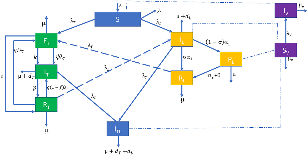
Figure 1. Compartment diagram of visceral leishmaniasis and tuberculosis co-infection. The dashed lines show that the infected sandflies (I_V) infect susceptible individuals (S). Individuals infected with VL (I_L), those who develop PKDL after the treatment of VL (P_L) and VL infected individuals having TB symptoms (I_TL) infect susceptible sandflies (S_V).

The parameters and their values of the model are summarized in Table 1.

TABLE 1

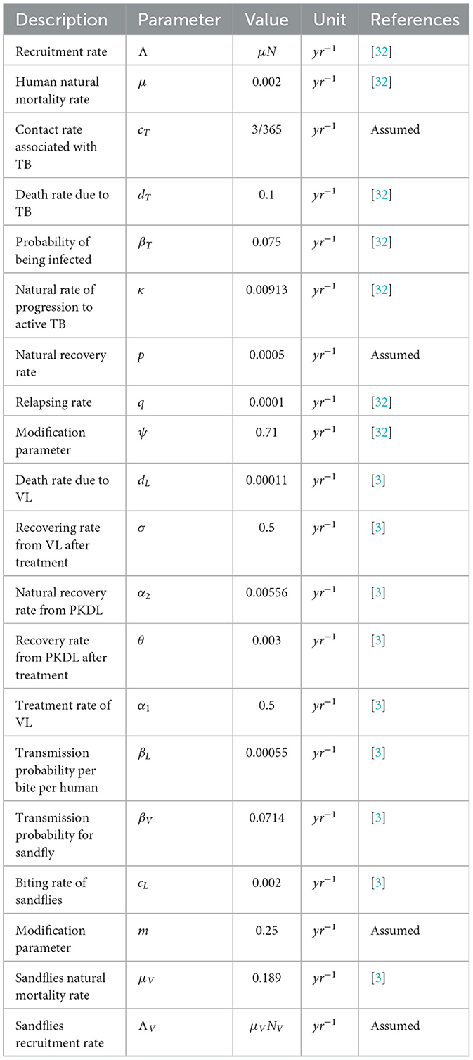
Table 1. Descriptions and values of parameters of the co-infection model (6).

2.3. Invariant region and positivity of solutions

The basic dynamical features of the co-infection model (6) are summarized in the following Lemma.

Lemma 1. Let (S, E_T, I_T, R_T, I_L, P_L, R_L, I_TL, S_V, I_V) be the solution of the co-infection model (6) with initial conditions (7). The closed set

$\begin{array}{l}\Omega ={\Omega }_H\times {\Omega }_V,\end{array}$

where

$\begin{array}{l}{\Omega }_H=\left\{(S+E_T+I_T+R_T+I_L+P_L+R_L+I_{TL})\in {ℝ}_{+}^8:N\le \frac{\Lambda }{\mu }\right\},\\ {\Omega }_V=\left\{(S_V+I_V)\in {ℝ}_{+}^2:N_V\le \frac{{\Lambda }_V}{{\mu }_V}\right\},\end{array}$

is positively invariant and attracting for the co-infection model (6).

Proof. Adding the first eight equations in system (6), we have

$\begin{array}{l}\frac{dN}{dt}=\Lambda -\mu N-d_T{I}_T-d_L{I}_L\\ \le \Lambda -\mu N.\end{array}$

The comparison theorem [33] can be used to show that

$\begin{array}{l}0\le N\le N(0)e^{-\mu t}+\frac{\Lambda }{\mu }(1-e^{-\mu t}).\end{array}$

Thus, as t → ∞, $0\le N\le \frac{\Lambda }{\mu }$. This implies that Ω_H is an attracting set with respect to the model (6). Similarly, adding the last two equations in system (6), we have

$\begin{array}{ll}\frac{d{N}_V}{dt}={\Lambda }_V-{\mu }_{V}N.& (8)\end{array}$

Similarly, it can be shown that as t → ∞, $0\le N_V\le \frac{{\Lambda }_V}{{\mu }_V}$ implying that Ω_V is an attracting set with respect to model (6).

Thus, it follows that all possible solutions of the model (6) will enter the region

$\begin{array}{l}\Omega ={\Omega }_H\times {\Omega }_V.\end{array}$

              □

Lemma 2. Let the initial data be as given in 7. Then, the solution set {S, E_T, I_T, R_T, I_L, P_L, R_L, I_TL, S_V, I_V} of system (6) is positive for all t > 0.

Proof. From the first equation of system (6), we have

$\begin{array}{l}\dot{S}=\Lambda -{\lambda }_{T}S-{\lambda }_{L}S-\mu S\\ \ge -{\lambda }_{T}S-{\lambda }_{L}S-\mu S.\end{array}$

Simple integration techniques yields

$\begin{array}{l}S(t)\ge S(0)e^{-({\lambda }_T+{\lambda }_L+\mu )t}>0\text{ since }{\lambda }_T+{\lambda }_L+\mu >0.\end{array}$

Similarly, it can be shown that the remaining variables are also positive for all t > 0. □

These lemmas verify that every solution of the co-infection model (6) with initial conditions in Ω remains there for t > 0. Furthermore, in Ω, the usual existence, uniqueness, and continuation results hold for the system so that the model system (6) is well posed mathematically and epidemiological. Thus, it is sufficient to consider the dynamics of the co-infection model (6) in Ω.

Next, we consider the dynamics of the two sub-models, namely, TB-only and VL-only models. This will help to lay down the foundation for the qualitative analysis of the full co-infection model.

3. TB sub-model

The TB sub-model is given by

$\begin{array}{ll}\{\begin{array}{l}\dot{S}=\Lambda -{\lambda }_{T}S-\mu S,\\ {\dot{E}}_T={\lambda }_{T}S-\kappa E_T-\psi {\lambda }_T{E}_T+fq{\lambda }_T{R}_T-\mu E_T,\\ {\dot{I}}_T=\kappa E_T+\psi {\lambda }_T{E}_T+q(1-f){\lambda }_T{R}_T-p{I}_T-(\mu +d_T)I_T,\\ {\dot{R}}_T=p{I}_T-qf{\lambda }_T{R}_T-q(1-f){\lambda }_T{R}_T-\mu R_T,\end{array}& (9)\end{array}$

with initial conditions (IC)

$\begin{array}{ll}S(0)>0,E_T(0)\ge 0,I_T(0)\ge 0,R_T(0)>0.& (10)\end{array}$

Here, the total human population is N_T = S + E_T + I_T + R_T. The parameters of the TB sub-model are as described in Table 1. The basic dynamical features of the TB sub-model model (9) are summarized in the following Lemma.

Lemma 3. Let the solution of system (9) be (S, E_T, I_T, R_T) with initial conditions (10). The closed set

$\begin{array}{ll}{\mathcal{G}}_{\mathcal{T}}={\displaystyle \{S,E_T,I_T,R_T\in {ℝ}_{\ge 0}:N_T\le \frac{\Lambda }{\mu }\}.}& (11)\end{array}$

is positively invariant and attracting under the flow governed by model system (9).

Proof. Adding all the equations in the system (9), we obtain

$\begin{array}{l}\frac{d{N}_T}{dt}=\Lambda -\mu N_T-d_T{I}_T,\\ \le \Lambda -\mu N_T.\end{array}$

The comparison theorem can be used to show that

$\begin{array}{l}0\le N_T\le N_T(0)e^{-\mu t}+\frac{\Lambda }{\mu }(1-e^{-\mu t}).\end{array}$

Thus, as t → ∞, $0\le N_T\le \frac{\Lambda }{\mu }$. This implies that ${\mathcal{G}}_{\mathcal{T}}$ is an attracting set with respect to model (9). □

3.1. TB sub-model disease-free equilibrium

The disease-free equilibrium (DFE) for the TB sub-model (9) is given by

$\begin{array}{ll}{E}_0={\displaystyle (S_0,E_{T_0},I_{T_0},R_{T_0})=(\frac{\Lambda }{\mu },0,0,0).}& (12)\end{array}$

According to the next-generation matrix approach in van den Driessche and Watmough [14], to compute the basic reproduction of the TB sub-model, we set $X={\left(E_T,I_T,R_T\right)}^T$ and rewrite the model (9) in the matrix form

$\begin{array}{ll}\frac{dX}{dt}=\mathcal{F}(X)-\mathcal{V}(X),& (13)\end{array}$

where

$\begin{array}{l}\mathcal{F}=\left[\begin{array}{c}{\lambda }_{T}S\\ 0\\ 0\end{array}\right]\text{and}\end{array}$

$\begin{array}{l}\mathcal{V}=\left[\begin{array}{c}\kappa E_T+\psi {\lambda }_T{E}_T-fq{\lambda }_T{R}_T+\mu E_T\\ -\kappa E_T-\psi {\lambda }_T{E}_T-q(1-f){\lambda }_T{R}_T+p{I}_T+(\mu +d_T)I_T\\ -p{I}_T+q(1-f){\lambda }_T{R}_T+\mu R_T\end{array}\right].\end{array}$

At the equilibrium point E₀, the Jacobian matrices of $\mathcal{F}$ and $\mathcal{V}$ are

$\begin{array}{l}F=\left[\begin{array}{ccc}0& {\beta }_T{c}_T& 0\\ 0& 0& 0\\ 0& 0& 0\end{array}\right]\text{and}V=\left[\begin{array}{ccc}\kappa +\mu & 0& 0\\ -k& p+\mu +d_T& 0\\ 0& -p& \mu \end{array}\right].\end{array}$

It follows that the TB sub-model reproduction number is given by

$\begin{array}{ll}{\mathcal{R}}_1=\frac{\kappa {\beta }_T{c}_T}{(\mu +\kappa )(\mu +d_T+p)}.& (14)\end{array}$

A value of ${\mathcal{R}}_1$ less than one indicates that TB will be eliminated while a value greater than one indicates that a TB infection will continue to spread within the susceptible hosts.

Theorem 1. The disease-free equilibrium point of the TB-only sub-model (9) is locally asymptotically stable if ${\mathcal{R}}_1<1$ and unstable otherwise.

Proof. The Jacobian matrix of model (9) at the disease-free equilibrium E₀ is

$\begin{array}{ll}{J}_0=\left(\begin{array}{cccc}-\mu & 0& -{\beta }_T{c}_T& 0\\ 0& -(\kappa +\mu )& {\beta }_T{c}_T& 0\\ 0& \kappa & -\left(p+\mu +d_T\right)& 0\\ 0& 0& p& -\mu \end{array}\right).& (15)\end{array}$

The characteristic equation of matrix J₀ is

$\begin{array}{ll}{(\lambda +\mu )}^2((\kappa +\lambda +\mu )(d_T+\lambda +\mu +p)-\kappa c_T{\beta }_T)=0,& (16)\end{array}$

where the eigenvalues can be obtained using the approach in [34]. Two eigenvalues of matrix J₀ are −μ (twice) and are both negative. The remaining two eigenvalues can be found by finding the eigenvalues of the sub-matrix

$\begin{array}{ll}A=\left(\begin{array}{cc}-\left(\kappa +\mu \right)& {\beta }_T{c}_T\\ \kappa & -\left(p+\mu +d_T\right)\end{array}\right).& (17)\end{array}$

By definition, the eigenvalues of matrix A are real and negative if tr(A) < 0 and det(A) > 0 (Routh-Hurwitz criterion). Thus, the trace and determinant of matrix A are

$\begin{array}{ll}\text{tr}(A)=-d_T-\kappa -2\mu -p,& (18)\end{array}$

$\begin{array}{l}\text{det}(A)=(\kappa +\mu )(d_T+\mu +p)-\kappa c_T{\beta }_T,\\ =(\kappa +\mu )(p+\mu +d_T)(1-{\mathcal{R}}_1),& (19)\end{array}$

respectively. Since all model parameters are assumed to be non-negative, it follows that tr(A) < 0 regardless of the value of ${\mathcal{R}}_1$. We also have that det(A) > 0 if and only if ${\mathcal{R}}_1<1$.

Therefore, we conclude that if ${\mathcal{R}}_1<1$, then tr(A) < 0 and det(A) > 0, implying that all the eigenvalues of matrix J₀ have a negative real part. The disease-free equilibrium ${\mathcal{R}}_1$ is locally asymptotically stable. If ${\mathcal{R}}_1\ge 1$, then det(A) ≤ 0, which proves the instability of E₀. □

3.2. Existence of the endemic equilibrium

The endemic equilibrium is the equilibrium (EE) of model (9) in which the infected component of the system is non-zero. The endemic equilibrium E₁ = (S_*, E_T*, I_T*, R_T*) in terms of the force of infection ${\mathrm{\lambda }}_T^{*}$ is given by

$\begin{array}{l}{S}_{*}=\frac{\Lambda }{{\lambda }_T^{*}+\mu },\\ E_{T*}=\frac{{\lambda }_T^{*}\Lambda (d_T(\mu +{\lambda }_T^{*}q)+f{\lambda }_T^{*}pq+\mu (\mu +p+{\lambda }_T^{*}q))}{({\lambda }_T^{*}+\mu )(d_T(\mu +{\lambda }_T^{*}q)(\kappa +{\lambda }_T^{*}\psi +\mu )+\mu (p(f{\lambda }_T^{*}q+\kappa +{\lambda }_T^{*}\psi +\mu )+(\mu +{\lambda }_T^{*}q)(\kappa +{\lambda }_T^{*}\psi +\mu )))},\\ I_{T*}=\frac{{\lambda }_T^{*}\Lambda (\kappa +{\lambda }_T^{*}\psi )(\mu +{\lambda }_T^{*}q)}{({\lambda }_T^{*}+\mu )(d_T(\mu +{\lambda }_T^{*}q)(\kappa +{\lambda }_T^{*}\psi +\mu )+\mu (p(f{\lambda }_T^{*}q+\kappa +{\lambda }_T^{*}\psi +\mu )+(\mu +{\lambda }_T^{*}q)(\kappa +{\lambda }_T^{*}\psi +\mu )))},\\ R_{T*}=\frac{{\lambda }_T^{*}\Lambda p(\kappa +{\lambda }_T^{*}\psi )}{({\lambda }_T^{*}+\mu )(d_T(\mu +{\lambda }_T^{*}q)(\kappa +{\lambda }_T^{*}\psi +\mu )+\mu (p(f{\lambda }_T^{*}q+\kappa +{\lambda }_T^{*}\psi +\mu )+(\mu +{\lambda }_T^{*}q)(\kappa +{\lambda }_T^{*}\psi +\mu )))},\end{array}$

where

$\begin{array}{ll}{\lambda }_T^{*}=\frac{{\beta }_T{c}_T{I}_{T*}}{N_{T*}}.& (20)\end{array}$

Substituting E₁ into Equation (20) and simplifying yields the cubic equation

$\begin{array}{ll}{a}_0{\lambda }_T^{*3}+a_1{\lambda }_T^{*2}+a_2{\lambda }_T^{*}+a_3=0,& (21)\end{array}$

where

$\begin{array}{l}{a}_0=q\psi ,\\ a_1=\psi (-{\beta }_T{c}_{T}q+\mu +p+\mu q)+q(\psi +1)d_T+q(fp+\kappa +\mu ),\\ a_2=-c_T{\beta }_T(\mu \psi +\kappa q)+d_T(\mu \psi +\mu +q(\kappa +\mu ))\\ +p(\mu (fq+\psi +1)+\kappa )+\mu (\mu \psi +(q+1)(\kappa +\mu )),\\ a_3=\mu (\mu +\kappa )(p+\mu +d_T)(1-{\mathcal{R}}_1).\end{array}$

Thus, the endemic equilibrium E₁ of the TB sub-model is obtained by solving Equation (21) for positive ${\lambda }_T^{*}$ and substituting back into the equations in E₁. The number of possible positive real roots of the cubic polynomial Equation (21) depends on the signs of a₀, a₁, a₂, and a₃. We investigate this by using the Descartes rule of signs. The rule asserts that the number of positive roots is at most the number of sign changes in the sequence of polynomial coefficients. The possibilities are illustrated in Table 2.

TABLE 2

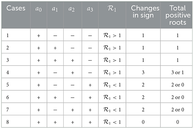
Table 2. Number of possible positive roots of the cubic polynomial (21).

The outcomes are established in the following theorem.

Theorem 2. The TB sub-model (9) has the following features:

1. A unique endemic equilibrium when ${\mathcal{R}}_1>1$ and cases 1–3 hold.

2. One or more endemic equilibrium when ${\mathcal{R}}_1>1$ and case 4 holds, as well as when ${\mathcal{R}}_1<1$ and cases 5-7 hold.

3. No endemic equilibrium when ${\mathcal{R}}_1<1$ and case 8 holds. This is the case when all coefficients are positive.

3.3. Backward bifurcation

For model (9), the existence of multiple TB persistence equilibria E₁ for ${\mathcal{R}}_1$ suggests the possibility of the backward bifurcation phenomenon. Epidemiologically, it suggests that ${\mathcal{R}}_1$ may not be sufficient to decide whether or not TB would persist in the population. Instead, it depends on the initial population size of the individuals when ${\mathcal{R}}_1<1$. We investigate and set a threshold for the presence of backward bifurcation in system (9).

From Theorem 1 and 2, we see that if we consider ${\mathcal{R}}_1$ as a bifurcation parameter, then there is an exchange of stability properties between equilibrium E₀ and E₁ at ${\mathcal{R}}_1=1$. We investigate the nature of bifurcation involving E₀ at ${\mathcal{R}}_1=1$ based on the use of the center manifold theory [15]. First, consider the case when ${\mathcal{R}}_1=1$ and solve for β_T to obtain

$\begin{array}{l}{\beta }_T={\beta }_T^{*}=\frac{(\kappa +\mu )(d_T+\mu +p)}{c_T\kappa }.\end{array}$

The ${\beta }_T={\beta }_T^{*}$ is chosen as the bifurcation parameter. Furthermore, the Jacobian of system (9) evaluated at E₀ with ${\beta }_T={\beta }_T^{*}$ is given by

$J\left({\text{E}}_0,{\beta }_T^{*}\right)=\left(\begin{array}{cccc}-\mu & 0& -\frac{\left(\kappa +\mu \right)\left(p+\mu +d_T\right)}{\kappa }& 0\\ 0& -\kappa -\mu & \frac{\left(\kappa +\mu \right)\left(p+\mu +d_T\right)}{\kappa }& 0\\ 0& \kappa & -p-\mu -d_T& 0\\ 0& 0& p& -\mu \end{array}\right).$

The $J\left({\text{E}}_0,{\beta }_T^{*}\right)$ has only one eigenvalue with zero real part. This then implies that the model (9) with ${\beta }_T={\beta }_T^{*}$ has at least one non-hyperbolic equilibrium point. We then use the center manifold approach to further analyze the dynamics of model (9). Corresponding to the zero eigenvalue, the Jacobian $J\left({\text{E}}_0,{\beta }_T^{*}\right)$ has a right eigenvector given by $w={\left(w_1,w_2,w_3,w_4\right)}^T$, where

$\begin{array}{l}{w}_1=-\frac{(\kappa +\mu )}{\mu }{w}_2,w_3=\frac{\kappa }{d_T+\mu +p}{w}_2,\\ w_4=\frac{\kappa p}{\mu (d_T+\mu +p)}{w}_2,w_2>0,\end{array}$

and a left eigenvector given by $v={\left(v_1,v_2,v_3,v_4\right)}^T$, where

$\begin{array}{l}{v}_1=v_4=0,v_3=\frac{\kappa +\mu }{\kappa }{v}_2,v_2>0.\end{array}$

We then follow the analysis as carried out by [16, 17]. Compute the coefficients $\widehat{a}$ and $\widehat{b}$ defined in theorem 4.1 by Castillo-Chavez and Song [15].

Computation of $\widehat{a}$ and $\widehat{b}$

The $\widehat{a}$ and $\widehat{b}$ are given by

$\begin{array}{l}\widehat{a}={\displaystyle \sum _{k,i,j=1}^4{v}_k{w}_i{w}_j\frac{{\partial }^2{f}_k}{\partial x_i\partial x_j}{|}_{{\text{E}}_0},}\\ \widehat{b}={\displaystyle \sum _{k,i=1}^4{v}_k{w}_i\frac{{\partial }^2{f}_k}{\partial x_i\partial {\beta }_T}{|}_{{\text{E}}_0}.}\end{array}$

We use the center manifold approach on the model system (9). Let S = x₁, E = x₂, I = x₃, and R = x₄. Then N = x₁ + x₂ + x₃ + x₄ so that

$\begin{array}{l}{x}_1^{\prime }=f_1=\Lambda -\frac{{\beta }_T{c}_T{x}_3{x}_1}{x_1+x_2+x_3+x_4}-\mu x_1,\\ x_2^{\prime }=f_2=\frac{{\beta }_T{c}_T{x}_3{x}_1}{x_1+x_2+x_3+x_4}-\kappa x_2-\frac{\psi {\beta }_T{c}_T{x}_3{x}_2}{x_1+x_2+x_3+x_4}\\ +\frac{qf\beta c{x}_3{x}_4}{x_1+x_2+x_3+x_4}-\mu x_2,\\ x_3^{\prime }=f_3=\kappa x_2+\frac{\psi {\beta }_T{c}_T{x}_3{x}_2}{x_1+x_2+x_3+x_4}+\frac{q(1-f){\beta }_T{c}_T{x}_3{x}_4}{x_1+x_2+x_3+x_4}\\ -p{x}_3-(\mu +d_T)x_3,\\ x_4^{\prime }=f_4=p{x}_3-\frac{qf{\beta }_T{c}_T{x}_3{x}_4}{x_1+x_2+x_3+x_4}-\frac{q(1-f){\beta }_T{c}_T{x}_3{x}_4}{x_1+x_2+x_3+x_4}-\mu x_4.\end{array}$

The associated non-zero partial derivatives of $f_i={\left(f_1,f_2,f_3,f_4\right)}^T$ at E₀ are given by

$\begin{array}{l}\frac{{\partial }^2{f}_2}{\partial x_2\partial x_3}=\frac{{\partial }^2{f}_2}{\partial x_3\partial x_2}=-\frac{c_T{\beta }_T\mu (1+\psi )}{\Lambda },\\ \frac{{\partial }^2{f}_2}{\partial x_3^2}=-\frac{2c_T{\beta }_T\mu }{\Lambda },\\ \frac{{\partial }^2{f}_2}{\partial x_3\partial x_4}=\frac{{\partial }^2{f}_2}{\partial x_4\partial x_3}=\frac{c_T(fq-1){\beta }_T\mu }{\Lambda },\\ \frac{{\partial }^2{f}_3}{\partial x_2\partial x_3}=\frac{{\partial }^2{f}_3}{\partial x_3\partial x_2}=\frac{c_T{\beta }_T\psi \mu }{\Lambda },\\ \frac{{\partial }^2{f}_3}{\partial x_3\partial x_4}=\frac{{\partial }^2{f}_3}{\partial x_4\partial x_3}=\frac{c_T(1-f){\beta }_{T}q\mu }{\Lambda }.\end{array}$

Using the above expressions, the coefficients $\widehat{a}$ is given by

$\begin{array}{l}\widehat{a}=v_2{\displaystyle \sum _{i,j=1}}{w}_i{w}_j\frac{{\partial }^2{f}_2}{\partial x_i\partial x_j}+v_3{\displaystyle \sum _{i,j=1}}{w}_i{w}_j\frac{{\partial }^2{f}_3}{\partial x_i\partial x_j}\\ =\frac{2\mu d_T}{\Lambda \left(\mu +d_T+p\right)}[\frac{\mu \psi {\beta }_T{c}_T}{d_T\left(\kappa +\mu \right)}\\ {\displaystyle -{\mathcal{R}}_1\left(1+\frac{\mu \left(\kappa +\mu \right)+p\left(\kappa -q\kappa +\mu -\left(1-f\right)q\mu \right)}{\mu d_T}\right)]v_2{w}_2^2.}\end{array}$

For the sign of $\widehat{b}$, we chose β_T as the bifurcation parameter and it can be shown that the associated non-zero partial derivatives of f_i at E₀ are given by

$\begin{array}{l}\frac{{\partial }^2{f}_1}{\partial x_3\partial {\beta }_T}=-c_T,\frac{{\partial }^2{f}_2}{\partial x_3\partial {\beta }_T}=c_T,\end{array}$

so that

$\begin{array}{l}\widehat{b}=v_2{w}_3\frac{{\partial }^2{f}_2}{\partial x_3\partial {\beta }_T}=\frac{c_T\kappa }{d_T+\mu +p}{v}_2{w}_2.\end{array}$

It is seen that $\widehat{b}$ is always positive, while $\widehat{a}$ can either be positive or negative. Depending on the signs of $\widehat{a}$ and $\widehat{b}$, we establish the following lemmas

Lemma 4. If $\widehat{a}$ < 0 and $\widehat{b}>0$, then the TB sub-model model (9) undergoes forward bifurcation which occurs at ${\mathcal{R}}_1=1$.

Lemma 5. If $\widehat{a}$ > 0 and $\widehat{b}>0$, then the TB sub-model model (9) undergoes backward bifurcation which occurs at ${\mathcal{R}}_1=1$.

Hence, the positivity of $\widehat{a}$ offers the threshold circumstance for the phenomenon of backward bifurcation.

4. Visceral leishmaniasis sub-model

The visceral leishmaniasis (VL) sub-model is given by

$\begin{array}{ll}\{\begin{array}{l}\dot{S}=\Lambda -{\lambda }_{L}S-\mu S,\\ {\dot{I}}_L={\lambda }_{L}S-\sigma {\alpha }_1{I}_L-(1-\sigma ){\alpha }_1{I}_L-(\mu +d_L)I_L,\\ {\dot{P}}_L=(1-\sigma ){\alpha }_1{I}_L-({\alpha }_2+\theta )P_L-\mu P_L,\\ {\dot{R}}_L=\sigma {\alpha }_1{I}_L+({\alpha }_2+\theta )P_L-\mu R_L,\\ \dot{S_V}={\Lambda }_V-{\lambda }_V{S}_V-{\mu }_V{S}_V,\\ \dot{I_V}={\lambda }_V{S}_V-{\mu }_V{I}_V.\end{array}& (22)\end{array}$

The force of VL infection in humans is ${\lambda }_L=\frac{{\beta }_L{c}_{L}m{I}_V}{N_L}$. Susceptible individuals are infected with visceral leishmaniasis following contact with infected sandflies at a per capita rate ${\lambda }_V=\frac{{\beta }_V{c}_L\left(I_L+P_L\right)}{N_L}$. Here, we have that the total human population is N_L = S + I_L + P_L + R_L. The total human population dynamics for the VL sub-model are given by

$\begin{array}{ll}\dot{N_L}=\Lambda -\mu N_L-d_L{I}_L.& (23)\end{array}$

Given that the initial conditions are non-negative, i.e., N_L(0) ≥ 0, the total human population is positive and bounded for all finite time t > 0. The dynamics of the sandflies population are given by

$\begin{array}{ll}\dot{N_V}={\Lambda }_V-{\mu }_V{N}_V.& (24)\end{array}$

We conclude that all feasible solutions for the human population enter the region

$\begin{array}{ll}{\mathcal{G}}_{\mathcal{L}}={\displaystyle \{S,I_L,P_L,R_L\in {ℝ}_{\ge 0}:0\le N_L\le \frac{\Lambda }{\mu }\}},& (25)\end{array}$

while feasible solutions for the sandflies population entering the region,

$\begin{array}{ll}{\mathcal{G}}_{\mathcal{V}}={\displaystyle \{S_V,I_V\in {ℝ}_{\ge 0}:0\le N_V\le \frac{{\Lambda }_V}{{\mu }_V}\}}.& (26)\end{array}$

4.1. The disease-free equilibrium

The disease-free equilibrium (DFE) for the VL-only model is given by

$\begin{array}{ll}{\mathcal{Q}}_0={\displaystyle (S,I_L,P_L,R_L,S_V,I_V)=(\frac{\Lambda }{\mu },0,0,0,\frac{{\Lambda }_V}{{\mu }_V},0)}.& (27)\end{array}$

According to the next-generation matrix approach, to compute the basic reproduction of the VL sub-model we set $X={\left(I_L,P_L,R_T,S,I_V,S_V\right)}^T$ and rewrite the model (22) in the matrix form

$\begin{array}{ll}\frac{dX}{dt}=\mathcal{F}(X)-\mathcal{V}(X),& (28)\end{array}$

where

$\begin{array}{l}\mathcal{F}=\left[\begin{array}{c}{\lambda }_{L}S\\ 0\\ {\lambda }_V{S}_V\end{array}\right]\text{and}\mathcal{V}=\left[\begin{array}{c}\sigma {\alpha }_1{I}_L+(1-\sigma ){\alpha }_1{I}_L+(\mu +d_L)I_L\\ ({\alpha }_2+\theta +\mu )P_L-(1-\sigma ){\alpha }_1{I}_L\\ {\mu }_V{I}_V\end{array}\right].\end{array}$

At the equilibrium point ${\mathcal{Q}}_0$, the Jacobian matrices of $\mathcal{F}$ and $\mathcal{V}$ are

$\begin{array}{l}F=\left[\begin{array}{ccc}0& 0& {\beta }_L{c}_{L}m\\ 0& 0& 0\\ \frac{\mu c_L{\beta }_V{\Lambda }_V}{\Lambda {\mu }_V}& \frac{\mu c_L{\beta }_V{\Lambda }_V}{\Lambda {\mu }_V}& 0\end{array}\right]\text{and}\\ V=\left[\begin{array}{ccc}{\alpha }_1+\mu +d_L& 0& 0\\ -(1-\sigma ){\alpha }_1& {\alpha }_2+\theta +\mu & 0\\ 0& 0& {\mu }_V\end{array}\right].\end{array}$

As such, the VL sub-model reproduction number is given by

$\begin{array}{ll}{\mathcal{R}}_2=\sqrt{\frac{\mu m{c}_L^2{\beta }_L{\beta }_V{\Lambda }_V({\alpha }_1(1-\sigma )+{\alpha }_2+\theta +\mu )}{\Lambda {\mu }_V^2({\alpha }_2+\theta +\mu )({\alpha }_1+d_L+\mu )}}.& (29)\end{array}$

Theorem 3. The disease-free equilibrium point of the VL-only sub-model (22) is locally asymptotically stable if ${\mathcal{R}}_2<1$ and unstable when ${\mathcal{R}}_2>1$.

Proof. The Jacobian of model (22) at the disease-free equilibrium ${\mathcal{Q}}_0$ is

$\begin{array}{ll}{J}_1=\left(\begin{array}{cccccc}-\mu & 0& 0& 0& 0& -{\beta }_L{c}_{L}m\\ 0& -\left(\mu +d_L+\left(1-\sigma \right){\alpha }_1+\sigma {\alpha }_1\right)& 0& 0& 0& {\beta }_L{c}_{L}m\\ 0& \left(1-\sigma \right){\alpha }_1& -\left({\alpha }_2+\theta +\mu \right)& 0& 0& 0\\ 0& \sigma {\alpha }_1& {\alpha }_2+\theta & -\mu & 0& 0\\ 0& -\frac{{\beta }_V{c}_L{\Lambda }_V\mu }{{\mu }_V\Lambda }& -\frac{{\beta }_V{c}_L{\Lambda }_V\mu }{{\mu }_V\Lambda }& 0& -{\mu }_V& 0\\ 0& \frac{{\beta }_V{c}_L{\Lambda }_V\mu }{{\mu }_V\Lambda }& \frac{{\beta }_V{c}_L{\Lambda }_V\mu }{{\mu }_V\Lambda }& 0& 0& -{\mu }_V\end{array}\right).& (30)\end{array}$

The matrix J₁ has three negative eigenvalues −μ (twice) and μ_V. The remaining eigenvalues are found by finding the eigenvalues of

$\begin{array}{ll}B=\left(\begin{array}{ccc}-\left(\mu +d_L+\left(1-\sigma \right){\alpha }_1+\sigma {\alpha }_1\right)& 0& {\beta }_L{c}_{L}m\\ \left(1-\sigma \right){\alpha }_1& -\left({\alpha }_2+\theta +\mu \right)& 0\\ \frac{{\beta }_V{c}_L{\Lambda }_V\mu }{{\mu }_V\Lambda }& -\frac{{\beta }_V{c}_L{\Lambda }_V\mu }{{\mu }_V\Lambda }& -{\mu }_V\end{array}\right).& (31)\end{array}$

The characteristic polynomial of B is

$\begin{array}{ll}{\lambda }^3+a_2{\lambda }^2+a_1\lambda +a_0=0,& (32)\end{array}$

where

$\begin{array}{l}{a}_2={\alpha }_1+{\alpha }_2+d_L+\theta +2\mu +{\mu }_V,\\ a_1=-\frac{\mu m{c}_L^2{\beta }_L{\beta }_V{\Lambda }_V}{\Lambda {\mu }_V}+({\alpha }_2+\theta +\mu )({\alpha }_1+d_L+\mu )\\ +{\mu }_V({\alpha }_1+{\alpha }_2+d_L+\theta +2\mu ),\\ a_0=(\mu +d_L+{\alpha }_1)(\theta +{\alpha }_2+\mu )\left[1-{\mathcal{R}}_2^2\right].\end{array}$

The Routh-Hurwitz criteria reveals that the roots of polynomial (32) have negative real parts if

$\begin{array}{l}{a}_0>0,a_2>0,a_2{a}_1>a_0.\end{array}$

We observe that a₂ > 0 always and a₀ > 0 if ${\mathcal{R}}_2<1$. With a simple expansion, we can show that a₂a₁ > a₀ (i.e., a₂a₁ − a₀ > 0) if ${\mathcal{R}}_2<1$. Therefore, the disease-free equilibrium ${\mathcal{Q}}_0$ is locally stable when ${\mathcal{R}}_2<1$. □

4.2. Existence of the endemic equilibrium

The endemic equilibrium of model (22) is given by ${\text{E}}_2=\left(\widehat{S},{\widehat{I}}_L,{\widehat{P}}_L,{\widehat{R}}_L,{\widehat{S}}_V,{\widehat{I}}_V\right)$ as functions of the forces of infection ${\widehat{\lambda }}_L$ and ${\widehat{\lambda }}_V$

$\begin{array}{l}\widehat{S}=\frac{\Lambda }{\mu +{\lambda }_L},\\ {\widehat{I}}_L=\frac{\Lambda {\lambda }_L}{(\mu +{\lambda }_L)({\alpha }_1+d_L+\mu )},\\ {\widehat{P}}_L=\frac{{\alpha }_1\Lambda (1-\sigma ){\lambda }_L}{({\alpha }_2+\theta +\mu )(\mu +{\lambda }_L)({\alpha }_1+d_L+\mu )},\\ {\widehat{R}}_L=\frac{{\alpha }_1\Lambda {\lambda }_L({\alpha }_2+\theta +\mu \sigma )}{\mu ({\alpha }_2+\theta +\mu )(\mu +{\lambda }_L)({\alpha }_1+d_L+\mu )},\\ {\widehat{S}}_V=\frac{{\Lambda }_v}{{\lambda }_v+{\mu }_v},\\ {\widehat{I}}_V=\frac{{\lambda }_v{\Lambda }_v}{{\mu }_v({\lambda }_v+{\mu }_v)},\end{array}$

where

$\begin{array}{ll}{\widehat{\lambda }}_L=\frac{{\beta }_L{c}_{L}m{\widehat{I}}_V}{{\widehat{N}}_L}\text{ and }{\widehat{\lambda }}_V=\frac{{\beta }_V{c}_L({\widehat{I}}_L+{\widehat{P}}_L)}{{\widehat{N}}_L}.& (33)\end{array}$

Substituting E₂ into Equation (33) and simplifying yields the quadratic equation

$\begin{array}{ll}a{\widehat{\lambda }}_L^2+b{\widehat{\lambda }}_L+c=0,& (34)\end{array}$

where

$\begin{array}{l}a=\Lambda ({\alpha }_1+\mu ){\mu }_v(\mu c_L{\beta }_v({\alpha }_1(1-\sigma )+{\alpha }_2+\theta +\mu )\\ +({\alpha }_1+\mu ){\mu }_v({\alpha }_2+\theta +\mu )),& (35)\end{array}$

$\begin{array}{l}b=\Lambda \mu {\mu }_v^2{\left({\alpha }_1+d_L+\mu \right)}^2\left({\alpha }_2+\theta +\mu \right)\\ \left[\frac{2\left(\mu +{\alpha }_1\right)}{{\alpha }_1+d_L+\mu }+{\mathcal{R}}_2^2\left(\frac{\Lambda {\mu }_v}{m{\beta }_L{c}_L{\Lambda }_v}-1\right)\right],& (36)\end{array}$

$\begin{array}{ll}c=\Lambda {\mu }^2{\mu }_v^2{({\alpha }_1+d_L+\mu )}^2({\alpha }_2+\theta +\mu )(1-{\mathcal{R}}_2^2).& (37)\end{array}$

Therefore, the endemic equilibrium E₂ of the VL sub-model (22) is obtained by solving Equation (34) for positive λ^* and substituting back into the equations in E₂. To find the solutions of Equation (34), we make the following observations: a is always positive, while b and c may be positive or negative depending on the signs of ${\mathcal{R}}_2$, i.e., we have

$\begin{array}{ll}a>0,b=\{\begin{array}{c}>0\\ <0\end{array}\text{ and }c=\{\begin{array}{cc}>0& \text{if}{\mathcal{R}}_2<1\\ <0& \text{if}{\mathcal{R}}_2>1.\end{array}& (38)\end{array}$

From Equation (38), five cases in determining the solution/roots of Equation (34) arise:

(i) Case 1: If ${\mathcal{R}}_2<1$, then c > 0 and so Equation (34) has two positive roots when b < 0.

(ii) Case 2: If ${\mathcal{R}}_2<1$, then c > 0 and so Equation (34) has no positive roots (two negative roots) when b < 0.

(iii) Case 3: If ${\mathcal{R}}_2>1$, then c < 0 and so Equation (34) has one positive root when b > 0.

(iv) Case 4: If ${\mathcal{R}}_2>1$, then c < 0 and so Equation (34) also has one positive root when b < 0.

(v) Case 5: When ${\mathcal{R}}_2=1$, Equation (34) reduces to ${\widehat{\lambda }}_L\left(a\widehat{\lambda }+b\right)=0$, at which ${\widehat{\lambda }}_L=0$ (corresponding to the disease-free equilibrium ${\mathcal{Q}}_0$) and ${\widehat{\lambda }}_L=\frac{-b}{a}$ is a positive root when b < 0 and negative root (biologically meaningless) when b > 0.

Furthermore, the critical value of ${\mathcal{R}}_2$ denoted by ${\mathcal{R}}_c$ in the case when ${\mathcal{R}}_2<1$ is found by setting the discriminant Δ = b² − 4ac to be zero. This yields

$\begin{array}{ll}{\mathcal{R}}_c=\sqrt{1-\frac{b^2}{4a\Lambda {\mu }^2{\mu }_v^2{({\alpha }_1+d_L+\mu )}^2({\alpha }_2+\theta +\mu )}}.& (39)\end{array}$

Thus, the following connections hold

• $\Delta <0\iff {\mathcal{R}}_2<{\mathcal{R}}_c$.

• $\Delta =0\iff {\mathcal{R}}_2={\mathcal{R}}_c$.

• $\Delta >0\iff {\mathcal{R}}_2>{\mathcal{R}}_c$.

It can be shown that backward bifurcation occurs for values of ${\mathcal{R}}_2$ such that ${\mathcal{R}}_c<{\mathcal{R}}_2<1$. The existence of the endemic equilibrium of model (22) is summarized as follows:

Theorem 4. The VL sub-model (22) has those as follows:

1. a unique endemic equilibrium if ${\mathcal{R}}_2>1$;

2. two endemic equilibria exists, one of which is locally stable, if b < 0 and ${\mathcal{R}}_2<1$;

3. otherwise, the DFE is the only unique attractor if ${\mathcal{R}}_2<1$.

From Theorems 3 and 4, model (22) has the usual bifurcation at ${\mathcal{R}}_2=1$. If we consider ${\mathcal{R}}_2$ as the bifurcation parameter, then by definition, there is a switch in stability properties between equilibrium point ${\mathcal{Q}}_0$ and E₂ at ${\mathcal{R}}_2=1$. Under certain conditions, model (22) exhibits a backward bifurcation, in which the endemic equilibrium exists for ${\mathcal{R}}_2<1$. Setting ${\mathcal{R}}_2=1$ and solving for β_L yields

$\begin{array}{l}{\beta }_L={\beta }_L^{*}=\frac{\Lambda {\mu }_v^2({\alpha }_2+\theta +\mu )({\alpha }_1+d_L+\mu )}{\mu m{c}_L^2{\beta }_v{\Lambda }_v({\alpha }_1(1-\sigma )+{\alpha }_2+\theta +\mu )},\end{array}$

and ${\beta }_L={\beta }_L^{*}$ is chosen as the bifurcation parameter.

Determining the conditions for the nature of bifurcation using center manifold theory follows as outlined in the sections above. The Jacobian of the system (22) evaluated at E₁ with ${\beta }_L={\beta }_L^{*}$ is given by

$J\left({\text{E}}_1,{\beta }_1^{*}\right)=\left(\begin{array}{cccccc}-\mu & 0& 0& 0& 0& -\frac{\Lambda \left(\mu +d_L+{\alpha }_1\right)\left(\theta +\mu +{\alpha }_2\right){\mu }_V^2}{\mu c_L\left(\theta +\mu \left(1-\sigma \right){\alpha }_1+{\alpha }_2\right){\beta }_V{\Lambda }_V}\\ 0& -\mu -d_L-\left(1-\sigma \right){\alpha }_1-\sigma {\alpha }_1& 0& 0& 0& \frac{\Lambda \left(\mu +d_L+{\alpha }_1\right)\left(\theta +\mu +{\alpha }_2\right){\mu }_V^2}{\mu c_L\left(\theta +\mu \left(1-\sigma \right){\alpha }_1+{\alpha }_2\right){\beta }_V{\Lambda }_V}\\ 0& \left(1-\sigma \right){\alpha }_1& -\theta -\mu -{\alpha }_2& 0& 0& 0\\ 0& \sigma {\alpha }_1& \theta +{\alpha }_2& -\mu & 0& 0\\ 0& -\frac{\mu c_L{\beta }_V{\Lambda }_V}{\Lambda {\mu }_V}& -\frac{\mu c_L{\beta }_V{\Lambda }_V}{\Lambda {\mu }_V}& 0& -{\mu }_V& 0\\ 0& \frac{\mu c_L{\beta }_V{\Lambda }_V}{\Lambda {\mu }_V}& \frac{\mu c_L{\beta }_V{\Lambda }_V}{\Lambda {\mu }_V}& 0& 0& -{\mu }_V\end{array}\right).$

The Jacobian $J\left({\text{E}}_1,{\beta }_L^{*}\right)$ has a right eigenvector given by $w={\left(w_1,w_2,w_3,w_4,w_5,w_6\right)}^T$, where

$\begin{array}{l}{w}_1=-\frac{({\alpha }_1+d_L+\mu )}{\mu }{w}_2,w_3=\frac{{\alpha }_1(1-\sigma )}{{\alpha }_2+\theta +\mu }{w}_2,\\ w_4=\frac{{\alpha }_1({\alpha }_2+\theta +\mu \sigma )}{\mu ({\alpha }_2+\theta +\mu )}{w}_2,w_2>0,\\ w_5=-\frac{\mu c_L{\beta }_V{\Lambda }_V({\alpha }_1(1-\sigma )+{\alpha }_2+\theta +\mu )}{\Lambda {\mu }_V^2({\alpha }_2+\theta +\mu )}{w}_2,\\ w_6=\frac{\mu c_L{\beta }_V{\Lambda }_V({\alpha }_1(1-\sigma )+{\alpha }_2+\theta +\mu )}{\Lambda {\mu }_V^2({\alpha }_2+\theta +\mu )}{w}_2,\end{array}$

and a left eigenvector given by $v={\left(v_1,v_2,v_3,v_4,v_5,v_6\right)}^T$, where,

$\begin{array}{l}{v}_1=v_4=v_5=0,v_3=\frac{({\alpha }_1+d_L+\mu )}{{\alpha }_1(1-\sigma )+{\alpha }_2+\theta +\mu }{v}_2,\\ v_6=\frac{\Lambda {\mu }_V({\alpha }_2+\theta +\mu )({\alpha }_1+d_L+\mu )}{\mu c_L{\beta }_V{\Lambda }_V({\alpha }_1(1-\sigma )+{\alpha }_2+\theta +\mu )}{v}_2,v_2>0.\end{array}$

Computation of $\widehat{a}$ and $\widehat{b}$

The $\widehat{a}$ and $\widehat{b}$ are given by

$\begin{array}{l}\widehat{a}={\displaystyle \sum _{k,i,j=1}^6{v}_k{w}_i{w}_j\frac{{\partial }^2{f}_k}{\partial x_i\partial x_j}{|}_{{\text{E}}_1},}\\ {\displaystyle \widehat{b}=\sum _{k,i=1}^6{v}_k{w}_i\frac{{\partial }^2{f}_k}{\partial x_i\partial {\beta }_L}{|}_{{\text{E}}_1}.}\end{array}$

We use the center manifold approach on the model system (22). Let S = x₁, I_L = x₂, P_L = x₃, R_L = x₄, S_V = x₅, and I_V = x₆. Then N = x₁ + x₂ + x₃ + x₄ and N_V = x₅ + x₆ so that

$\begin{array}{l}{x}_1^{\prime }=f_1=\Lambda -\frac{{\beta }_L{c}_{L}m{x}_6{x}_1}{x_1+x_2+x_3+x_4}-\mu x_1,\\ x_2^{\prime }=f_2=\frac{{\beta }_L{c}_{L}m{x}_6{x}_1}{x_1+x_2+x_3+x_4}-\sigma {\alpha }_1{x}_2\\ -(1-\sigma ){\alpha }_1{x}_2-(\mu +d_L)x_2,\\ x_3^{\prime }=f_3=(1-\sigma ){\alpha }_1{x}_2-({\alpha }_2+\theta )x_3-\mu x_3,\\ x_4^{\prime }=f_4=\sigma {\alpha }_1{x}_2+({\alpha }_2+\theta )x_3-\mu x_4,\\ x_5^{\prime }=f_5={\Lambda }_L-\frac{{\beta }_V{c}_L(x_2+x_3)x_5}{x_1+x_2+x_3+x_4}-{\mu }_V{x}_5,\\ x_6^{\prime }=f_6=\frac{{\beta }_V{c}_L(x_2+x_3)x_5}{x_1+x_2+x_3+x_4}-{\mu }_V{x}_6.\end{array}$

The associated non-zero partial derivatives of $f_i={\left(f_1,f_2,f_3,f_4,f_5,f_6\right)}^T$ at E₁ are given by

$\begin{array}{l}\frac{{\partial }^2{f}_2}{\partial x_2\partial x_6}=\frac{{\partial }^2{f}_2}{\partial x_3\partial x_6}=\frac{{\partial }^2{f}_2}{\partial x_4\partial x_6}=\frac{{\partial }^2{f}_2}{\partial x_6\partial x_2}=\frac{{\partial }^2{f}_2}{\partial x_6\partial x_3}\\ =\frac{{\partial }^2{f}_2}{\partial x_6\partial x_4}=-\frac{\mu m{c}_L{\beta }_L}{\Lambda },\\ \frac{{\partial }^2{f}_6}{\partial x_1\partial x_1}=\frac{{\partial }^2{f}_6}{\partial x_1\partial x_3}=\frac{{\partial }^2{f}_6}{\partial x_2\partial x_1}=\frac{{\partial }^2{f}_6}{\partial x_2\partial x_4}=\frac{{\partial }^2{f}_6}{\partial x_3\partial x_1}\\ =\frac{{\partial }^2{f}_6}{\partial x_3\partial x_4}=\frac{{\partial }^2{f}_6}{\partial x_4\partial x_2}=\frac{{\partial }^2{f}_6}{\partial x_4\partial x_3}=-\frac{{\mu }^2{c}_L{\beta }_V{\Lambda }_V}{{\Lambda }^2{\mu }_V},\\ \frac{{\partial }^2{f}_6}{\partial x_2\partial x_2}=\frac{{\partial }^2{f}_6}{\partial x_2\partial x_3}=\frac{{\partial }^2{f}_6}{\partial x_3\partial x_2}=\frac{{\partial }^2{f}_6}{\partial x_3\partial x_3}=-\frac{2{\mu }^2{c}_L{\beta }_V{\Lambda }_V}{{\Lambda }^2{\mu }_V},\\ \frac{{\partial }^2{f}_6}{\partial x_2\partial x_5}=\frac{{\partial }^2{f}_6}{\partial x_3\partial x_5}=\frac{{\partial }^2{f}_6}{\partial x_5\partial x_2}=\frac{{\partial }^2{f}_6}{\partial x_5\partial x_3}=\frac{\mu c_L{\beta }_L}{\Lambda }.\end{array}$

Using the above expressions, the coefficients $\widehat{a}$ is given by

$\begin{array}{l}\widehat{a}=v_2{\displaystyle \sum _{i,j=1}}{w}_i{w}_j\frac{{\partial }^2{f}_2}{\partial x_i\partial x_j}+v_6{\displaystyle \sum _{i,j=1}}{w}_i{w}_j\frac{{\partial }^2{f}_6}{\partial x_i\partial x_j}\\ =\frac{2v_2{w}_2^2{d}_L(\mu +d_L+{\alpha }_1)}{\Lambda }\\ \left[1-\frac{(\mu +{\alpha }_1)}{d_L}{\mathcal{R}}_2-\frac{\mu c_L{\beta }_V(\theta +\mu +(1-\sigma ){\alpha }_1+{\alpha }_2)}{{\mu }_V(\theta +\mu +{\alpha }_2)}\right].\end{array}$

For the sign of $\widehat{b}$, we chose β_L as the bifurcation parameter. The associated non-zero partial derivatives of f_i at E₁ are given by

$\begin{array}{l}\frac{{\partial }^2{f}_1}{\partial x_6\partial {\beta }_L}=-m{c}_L,\frac{{\partial }^2{f}_2}{\partial x_6\partial {\beta }_L}=m{c}_L,\end{array}$

so that

$\begin{array}{l}\widehat{b}=v_2{w}_6\frac{{\partial }^2{f}_2}{\partial x_6\partial {\beta }_L}\\ =\frac{\mu m{c}_L^2{\beta }_V{\Lambda }_V({\alpha }_1(1-\sigma )+{\alpha }_2+\theta +\mu )}{\Lambda {\mu }_V^2({\alpha }_2+\theta +\mu )}{v}_2{w}_2.\end{array}$

It is seen that $\widehat{b}$ is always positive, while $\widehat{a}$ can either be positive or negative. Depending on the signs of $\widehat{a}$ and $\widehat{b}$, we establish the following lemmas:

Lemma 6. If $\widehat{a}$ < 0 and $\widehat{b}>0$, then the VL sub-model model (22) undergoes forward bifurcation which occurs at ${\mathcal{R}}_2=1$.

Lemma 7. If $\widehat{a}$ > 0 and $\widehat{b}>0$, then the VL sub-model model (22) undergoes backward bifurcation which occurs at ${\mathcal{R}}_2=1$.

Hence, the positivity of $\widehat{a}$ offers the threshold circumstance for the phenomenon of backward bifurcation.

5. The full visceral leishmaniasis and tuberculosis co-infection model

In this section, we investigate the dynamical properties of the model (6). For convenience, we introduce the following new parameters:

$\begin{array}{ll}\begin{array}{l}{\zeta }_1=\kappa +\mu ,\\ {\zeta }_2=p+\mu +d_L,\\ {\zeta }_3={\alpha }_1+\mu +d_L,\\ {\zeta }_4={\alpha }_2+\theta +\mu ,\\ {\zeta }_5=\mu +d_T+d_L.\end{array}& (40)\end{array}$

5.1. The disease-free equilibrium

The disease-free equilibrium (EE) of the full model (6) is given as

$\begin{array}{r}{E}_{F1}={\displaystyle (S,E_T,I_T,R_T,I_L,P_L,R_L,I_{TL},S_V,I_V)}\\ ={\displaystyle (\frac{\Lambda }{\mu },0,0,0,0,0,0,0,\frac{{\Lambda }_V}{{\mu }_V},0)}.& (41)\end{array}$

We now use the next-generation matrix approach to compute the basic reproduction of the model (6). For this purpose, we set $X={\left(E_T,I_T,R_T,I_L,P_L,R_T,I_{TL},S,I_V,S_V\right)}^T$ and rewrite the model (6) in the matrix form

$\begin{array}{ll}\frac{dX}{dt}=\mathcal{F}(X)-\mathcal{V}(X),& (42)\end{array}$

where

$\begin{array}{cc}\mathcal{F}& =\left(\begin{array}{c}{\lambda }_{T}S\\ 0\\ 0\\ {\lambda }_{L}S+{\lambda }_L{R}_T\\ 0\\ 0\\ 0\\ 0\\ {\lambda }_V{S}_V\\ 0\end{array}\right),\text{and}\\ \mathcal{V}& =\left(\begin{array}{c}{\zeta }_1{E}_T+\psi {\lambda }_T{E}_T-qf{\lambda }_T{R}_T-{\lambda }_T{R}_L\\ -\kappa E_T-\psi {\lambda }_T{E}_T-q\left(1-f\right){\lambda }_T{R}_T+{\zeta }_2{I}_T+{\lambda }_L{I}_T\\ -p{I}_T-ϵE_T+qf{\lambda }_T{R}_T+q\left(1-f\right){\lambda }_T{R}_T+{\lambda }_L{R}_T+\mu R_T\\ {\zeta }_3{I}_L+{\lambda }_T{I}_L\\ -\left(1-\sigma \right){\alpha }_1{I}_L+{\zeta }_4{P}_L\\ -\sigma {\alpha }_1{I}_L+{\lambda }_T{R}_L-\left({\alpha }_2+\theta \right)P_L+\mu R_L\\ -{\lambda }_L{I}_T-{\lambda }_T{I}_L+{\zeta }_5{I}_{TL}\\ -\Lambda +{\lambda }_{T}S+{\lambda }_{L}S+\mu S\\ {\mu }_V{I}_V\\ -{\Lambda }_V+{\lambda }_V{S}_V+{\mu }_V{S}_V\end{array}\right)& (43)\end{array}$

We carry out the remainder of the calculations as before. The dominant eigenvalues of FV⁻¹ are

$\begin{array}{ll}\{\begin{array}{l}{\mathcal{R}}_1=\frac{{\beta }_T{c}_T\kappa }{(\mu +\kappa )(\mu +d_T+p)},\\ {\mathcal{R}}_2=\sqrt{\frac{\mu m{c}_L^2{\beta }_L{\beta }_V{\Lambda }_V({\alpha }_1(1-\sigma )+{\alpha }_2+\theta +\mu )}{\Lambda {\mu }_V^2({\alpha }_2+\theta +\mu )({\alpha }_1+d_L+\mu )}}.\end{array}& (44)\end{array}$

and these correspond to the reproduction numbers for the TB transmission model and the leishmaniasis transmission model, respectively. Thus, the basic reproduction number, ${\mathcal{R}}_0$, for the full model (6) is given by

$\begin{array}{ll}{\mathcal{R}}_0=max\left\{{\mathcal{R}}_1,{\mathcal{R}}_2\right\}.& (45)\end{array}$

Theorem 5. The disease-free equilibrium point E_F1 of the full model (6) is locally asymptotically stable if ${\mathcal{R}}_0<1$ and unstable when ${\mathcal{R}}_0>1$.

5.2. Bifurcation parameters

The TB and VL-only sub-models are shown to exhibit the phenomenon of backward bifurcation and consequently, the full co-infection model will exhibit the same feature. Below, we derive the bifurcation parameters for the full co-infection model (6). Let S = x₁, E_T = x₂, I_T = x₃, R_T = x₄, I_L = x₅, P_L = x₆, R_L = x₇, I_TL = x₈, S_V = x₉, and I_V = x₁₀. Hence,

$\begin{array}{ll}{N}^c=x_1+x_2+x_3+x_4+x_5+x_6+x_7+x_8,& (46)\end{array}$

$\begin{array}{ll}{N}_V^c=x_9+x_{10}.& (47)\end{array}$

Letting $X={\left(x_1,x_2,\dots ,x_{10}\right)}^T$, the full co-infection model (6) can be written in the form $\frac{dX}{dt}=F\left(X\right)$, where F = (f₁, f₂, …, f₁₀), as

$\begin{array}{l}{\dot{x}}_1=f_1=\Lambda -{\lambda }_T^c{x}_1-{\lambda }_L^c{x}_1-\mu x_1,\\ {\dot{x}}_2=f_2={\lambda }_T^c{x}_1-\kappa x_2-\psi {\lambda }_T^c{x}_2+qf{\lambda }_T^c{x}_4+{\lambda }_T^c{x}_7-\mu x_2,\\ {\dot{x}}_3=f_3=\kappa x_2+\psi {\lambda }_T^c{x}_2+q(1-f){\lambda }_T^c{x}_4-p{x}_3-{\lambda }_L^c{x}_3\\ -(\mu +d_T)x_3,\\ {\dot{x}}_4=f_4=p{x}_3-qf{\lambda }_T^c{x}_4-q(1-f){\lambda }_T^c{x}_4-{\lambda }_L{x}_4-\mu x_4,\\ {\dot{x}}_5=f_5={\lambda }_L^c{x}_1+{\lambda }_L^c{x}_4-\sigma {\alpha }_1{x}_5-(1-\sigma ){\alpha }_1{x}_5-{\lambda }_T^c{x}_5\\ -(\mu +d_L)x_5,\\ {\dot{x}}_6=f_6=(1-\sigma ){\alpha }_1{x}_5-({\alpha }_2+\theta )x_6-\mu x_6,\\ {\dot{x}}_7=f_7=\sigma {\alpha }_1{x}_5-{\lambda }_T^c{x}_7+({\alpha }_2+\theta )x_6-\mu x_7,\\ {\dot{x}}_8=f_8={\lambda }_L^c{x}_3+{\lambda }_T^c{x}_5-(\mu +d_T+d_L)x_8,\\ {\dot{x}}_9=f_9={\Lambda }_V-{\lambda }_V^c{x}_9-{\mu }_V{x}_9,\\ {\dot{x}}_{10}=f_{10}={\lambda }_V^c{x}_9-{\mu }_V{x}_{10},\end{array}$

and

$\begin{array}{r}{\lambda }_T^c=\frac{{\beta }_T{c}_T{x}_3}{N^c},{\lambda }_L^c=\frac{{\beta }_L{c}_{L}m{x}_{10}}{N^c},\text{and}\\ {\lambda }_V^c=\frac{{\beta }_v{c}_L(x_5+x_6)}{N^c}.\end{array}$

The Jacobian matrix of the system above at the DFE point E_F1 is given by

$\begin{array}{ll}{J}_{F1}=\left(\begin{array}{cccccccccc}-\mu & 0& -{\beta }_T{c}_T& 0& 0& 0& 0& 0& 0& -{\beta }_L{c}_{L}m\\ 0& -{\zeta }_1& {\beta }_T{c}_T& 0& 0& 0& 0& 0& 0& 0\\ 0& \kappa & -{\zeta }_2& 0& 0& 0& 0& 0& 0& 0\\ 0& 0& p& -\mu & 0& 0& 0& 0& 0& 0\\ 0& 0& 0& 0& -{\zeta }_3& 0& 0& 0& 0& {\beta }_L{c}_{L}m\\ 0& 0& 0& 0& \left(1-\sigma \right){\alpha }_1& -{\zeta }_4& 0& 0& 0& 0\\ 0& 0& 0& 0& \sigma {\alpha }_1& {\alpha }_2+\theta & -\mu & 0& 0& 0\\ 0& 0& 0& 0& 0& 0& 0& -{\zeta }_5& 0& 0\\ 0& 0& 0& 0& -\frac{\mu c_L{\beta }_V{\Lambda }_V}{\Lambda {\mu }_V}& -\frac{\mu c_L{\beta }_V{\Lambda }_V}{\Lambda {\mu }_V}& 0& 0& -{\mu }_V& 0\\ 0& 0& 0& 0& \frac{\mu c_L{\beta }_V{\Lambda }_V}{\Lambda {\mu }_V}& \frac{\mu c_L{\beta }_V{\Lambda }_V}{\Lambda {\mu }_V}& 0& 0& 0& -{\mu }_V\end{array}\right).& (48)\end{array}$

By computing the eigenvalues of the Jacobian J_F1, it can be shown that ${\mathcal{R}}_0=max\left\{{\mathcal{R}}_1,{\mathcal{R}}_2\right\}$, where ${\mathcal{R}}_1$ and ${\mathcal{R}}_2$ are as previously defined. ${\mathcal{R}}_0=max\left\{{\mathcal{R}}_1,{\mathcal{R}}_2\right\}$, hence, there is no competitive exclusion and the two diseases amplify each other. Thus, when ${\mathcal{R}}_1>1$ and ${\mathcal{R}}_2>1$, there is always co-existence no matter which of the reproduction numbers is greater. Although ${\mathcal{R}}_0$ does not combine the two reproduction numbers, by only studying the two diseases in isolation, we would miss the dual TB-visceral leishmaniasis co-infection, which has different dynamics to that of TB-only and visceral leishmaniasis only sub-models. Some additional insights are derived from studying the interaction of the two diseases, hence the full model. If $max\left\{{\mathcal{R}}_1,{\mathcal{R}}_2\right\}={\mathcal{R}}_1$, then, from Theorem 2, the TB-VL co-infection model exhibits backward bifurcation for values of ${\mathcal{R}}_1$ such that Lemma 5 holds.

On the contrary, if $max\left\{{\mathcal{R}}_1,{\mathcal{R}}_2\right\}={\mathcal{R}}_2$, and choosing β_L as the bifurcation parameter, then, the phenomenon of backward bifurcation occurs for values of ${\mathcal{R}}_2$ such that Lemma 7 holds. Consequently, the full model will also exhibit the phenomenon of backward bifurcation when ${\mathcal{R}}_0=1$.

5.3. Endemic equilibrium

The endemic equilibrium E₄ of the full model system (6) is given by

$\begin{array}{cc}{S}_2& =\frac{\Lambda }{{\lambda }_T^{*}+{\lambda }_L^{*}+\mu },\\ I_{T2}& =\frac{(\kappa +\psi )(q{\lambda }_T^{*}+{\lambda }_L^{*}+\mu )E_{T2}}{(q{\lambda }_T^{*}+{\lambda }_L^{*}+\mu )(p+{\lambda }_L^{*}+\mu +d_T)-q(1-f)p{\lambda }_T^{*}},\\ & R_{T2}=\\ & \frac{p(\kappa +\psi )(q{\lambda }_T^{*}+{\lambda }_L^{*}+\mu )E_{T2}}{{\displaystyle (q{\lambda }_T^{*}+{\lambda }_L^{*}+\mu )[(q{\lambda }_T^{*}+{\lambda }_L^{*}+\mu )(p+{\lambda }_L^{*}+\mu +d_T)-q(1-f)p{\lambda }_T^{*}]}},\\ I_{L2}& =\frac{{\lambda }_L^{*}{S}_2+{\lambda }_L^{*}{R}_{T2}}{{\alpha }_1+{\lambda }_T^{*}+\mu +d_T},\\ P_{L2}& =\frac{{\alpha }_1(1-\sigma )({\lambda }_L^{*}{S}_2+{\lambda }_L^{*})}{({\alpha }_2+\theta +\mu )({\alpha }_1+{\lambda }_T^{*}+\mu +d_T)},\\ R_{L2}& =\frac{\sigma {\alpha }_1{I}_{L2}+({\alpha }_2+\theta )P_{L2}}{{\lambda }_T^{*}+\mu },\\ I_{TL2}& =\frac{{\lambda }_L^{*}{I}_{T2}+{\lambda }_T^{*}{I}_{L2}}{\mu +d_T+d_L},\\ S_{V2}& =\frac{{\Lambda }_V}{{\mu }_V+{\lambda }_V^{*}},\\ I_{V2}& =\frac{{\lambda }_V^{*}{\Lambda }_V}{({\mu }_V+{\lambda }_V^{*}){\mu }_V}.\end{array}$

Solving for E_T2 in

$\begin{array}{l}{\lambda }_T^{*}{S}_2-(\kappa +\psi {\lambda }_T^{*}+\mu )E_{T2}+qf{\lambda }_T^{*}{R}_{T2}+{\lambda }_T^{*}{R}_{L2}=0.\end{array}$

The forces of infection at E₄ are given by,

$\begin{array}{r}{\lambda }_T^{*}=\frac{{\beta }_T{c}_T{I}_{T2}}{N^c},{\lambda }_L^{*}=\frac{{\beta }_L{c}_{L}m{I}_{V2}}{N^c},\text{and}\\ {\lambda }_V^{*}=\frac{{\beta }_V{c}_L(I_{L2}+I_{TL2}+P_{L2})}{N^c}.\end{array}$

6. Simulations and results

In this section, we provide simulation results for the TB-only model in Figure 2, the VL-only model in Figure 3, and the full VL-TB co-infection model in Figure 4. We performed the simulations using the in-built function ODE45 in MATLAB (MathWorks, Natick, MA, USA) [35], with the aim of understanding the long-term dynamics of the models and checking if it is consistent with the theoretical results. For this purpose, we used the parameter values given in Table 1. We observe from Figures 2–4 that the DFE points are locally asymptotically stable for each model. For the TB-only model, ${\mathcal{R}}_1<1$ and hence, the DFE point ${\text{E}}_0={\displaystyle (S_0,E_{T_0},I_{T_0},R_{T_0})=(\frac{\mathrm{\Lambda }}{\mu },0,0,0)}$ is locally asymptotically stable. This implies that the epidemic will be eradicated. The solutions of the model 9 are depicted in Figure 2. Similarly, the VL-only model DFE point ${\mathcal{Q}}_0={\displaystyle (S,I_L,P_L,R_L,S_V,I_V)=(\frac{\mathrm{\Lambda }}{\mu },0,0,0,\frac{{\mathrm{\Lambda }}_V}{{\mu }_V},0)}$ is locally asymptotically stable. This implies that the epidemic will be eradicated ${\mathcal{R}}_2<1$ as depicted in 1. Therefore, Figures 2–4 are consistent with theoretical results obtained for each case, and these results imply that the disease will be eliminated.

FIGURE 2

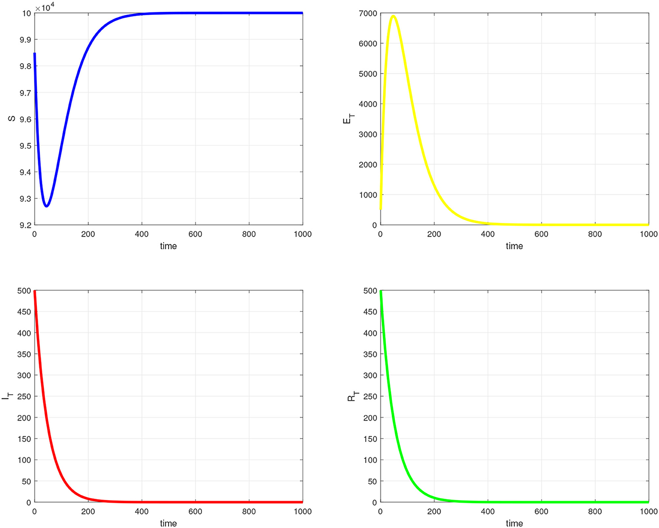
Figure 2. Simulation of tuberculosis sub-model.

FIGURE 3

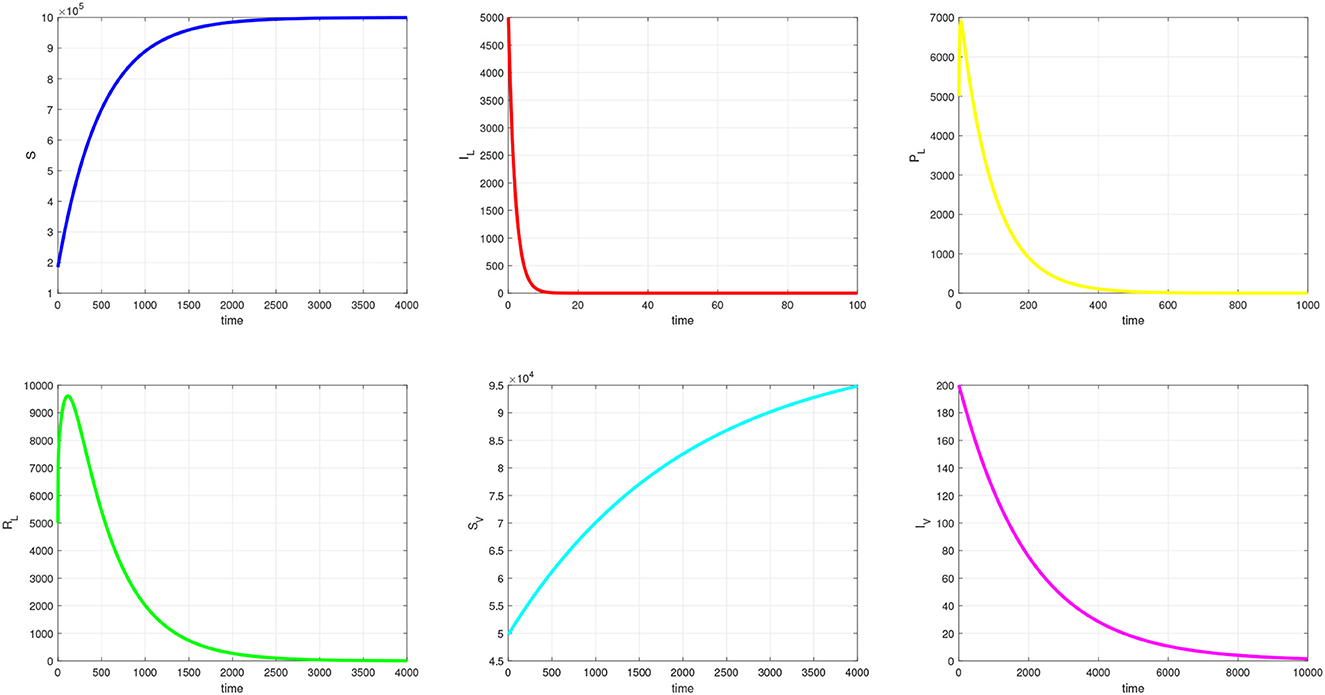
Figure 3. Simulation of visceral leishmaniasis sub-model.

FIGURE 4

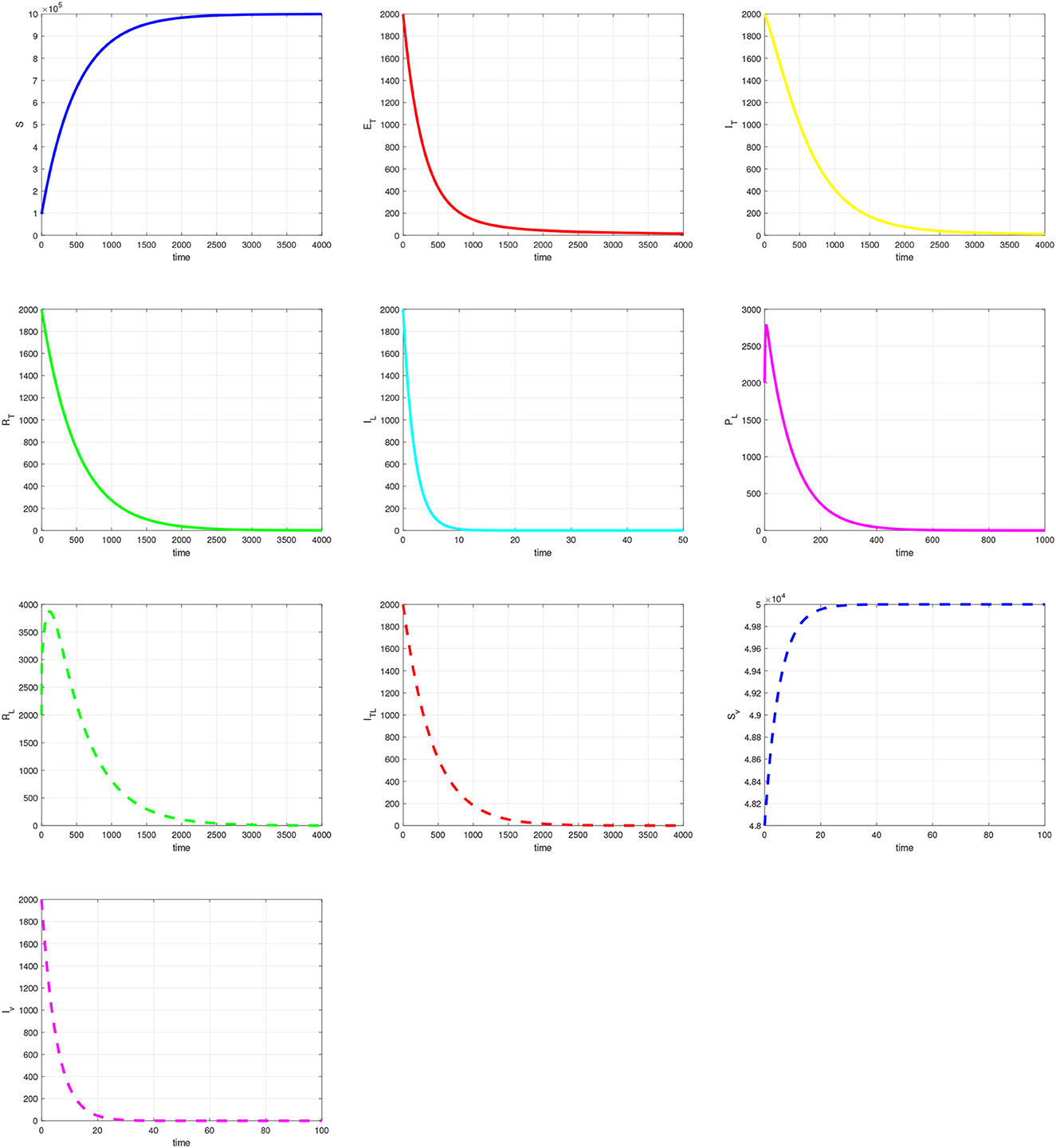
Figure 4. Simulation of the full visceral leishmaniasis and tuberculosis co-infection model.

6.1. Bifurcation analysis

6.1.1. TB-only model

The combined effect of β_T and d_T on the values of ${\mathcal{R}}_1$ are explored next to determine the threshold conditions of these parameters at which the TB-only model exhibits backwards and forward bifurcations. The ${\mathcal{R}}_1$ contours, see Figure 5, show an increase in ${\mathcal{R}}_1$ as β_T and d_T increase.

FIGURE 5

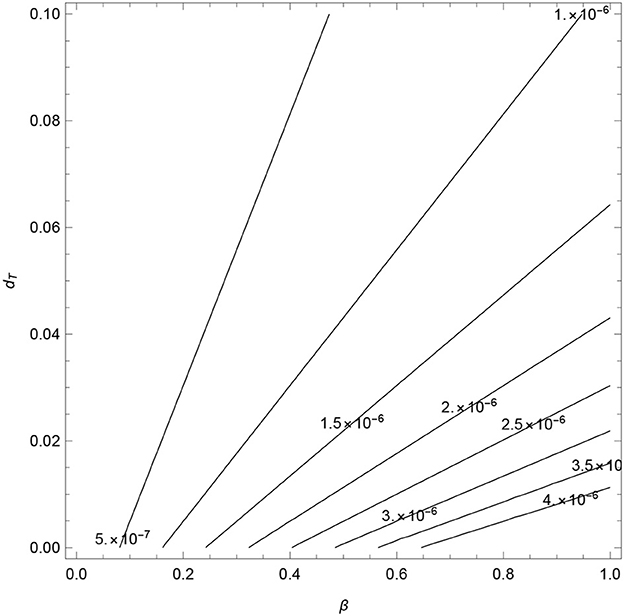
Figure 5. Contour plots of ${\mathcal{R}}_1$ as a function of transmission rate (β_T) and disease-induced death rate (d_T).

6.1.2. VL-only model

The combined effect of β_L, d_L, σ, α₁, and α₂ on the values of ${\mathcal{R}}_2$ are explored next to determine the threshold conditions of these parameters at which the VL-only model exhibits backward and forward bifurcations.

The ${\mathcal{R}}_2$ contours, see Figure 6, show an increase in ${\mathcal{R}}_2$ as β_L increases and d_L decreases. In Figure 7, we observe that ${\mathcal{R}}_2$ decrease as σ₁, α₁, and α₂ increase. All the ${\mathcal{R}}_2$ contours are less than unity, which signifies that these values of σ₁, α₁, and α₂ (and other fixed parameters) will lead to the elimination of VL from the community (in line with Theorem 3). However, the analysis verifies that the parameters σ₁, α₁, and α₂ are the cause of occurring backward bifurcation in the VL model whenever ${\mathcal{R}}_2<1$ as guaranteed by Lemma 6-7.

FIGURE 6

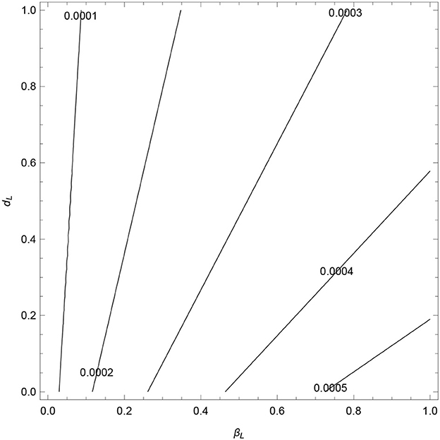
Figure 6. Contour plots of ${\mathcal{R}}_2$ as a function of transmission rate (β_L) and disease-induced death rate (d_L).

FIGURE 7

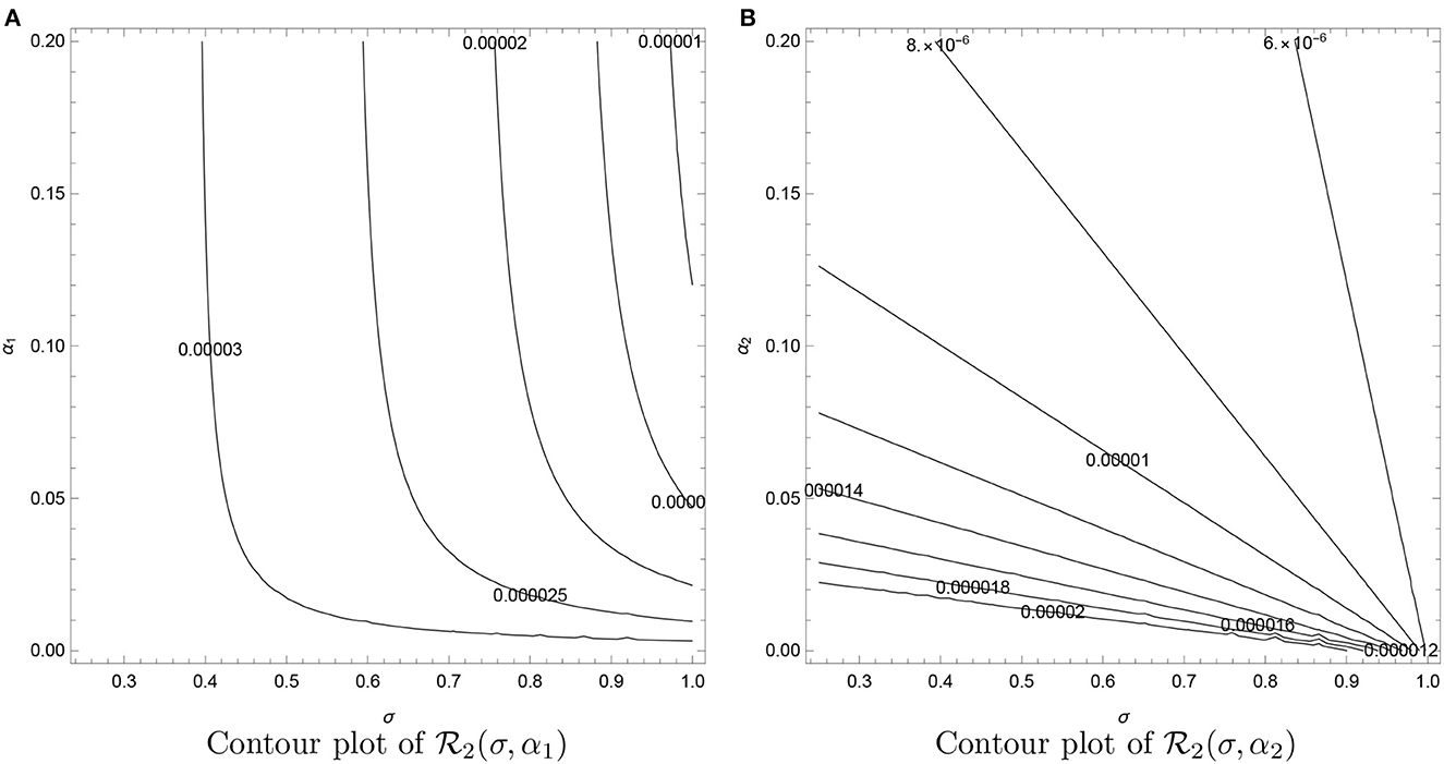
Figure 7. Contour plots of ${\mathcal{R}}_2$ as functions of recovery rate after treatment (σ), treatment rate (α₁), and recovery rate from PKDL (α₂). (A) Contour plot of ${\mathcal{R}}_2\left(\sigma ,{\alpha }_1\right)$. (B) Contour plot of ${\mathcal{R}}_2\left(\sigma ,{\alpha }_2\right)$.

7. Conclusion

In developing nations, visceral leishmaniasis (VL) and tuberculosis (TB) co-infection is becoming a growing public health concern. Leishmaniasis infection alters the protective immunologic response to Bacillus Calmette-Guerin (BCG) vaccine against tuberculosis [36]. Tuberculosis is an immuno-suppressive disease that causes latent leishmaniasis to proceed to clinical leishmaniasis, and VL can provoke latent TB infection to TB disease [36]. In this study, we developed and analyzed a model that describes transmission dynamics of visceral leishmaniasis and tuberculosis co-infection. Firstly, we analyzed the VL and TB sub-models separately. The reproduction number for each sub-model was calculated by the next-generation matrix approach. The local stability properties of the sub-models were studied. We observed that when the associated reproduction numbers (${\mathcal{R}}_1$) for the TB-only model and (${\mathcal{R}}_2$) for the VL-only are less than unity, respectively, the model exhibits bifurcation. We observed that ${\mathcal{R}}_0=max\left\{{\mathcal{R}}_1,{\mathcal{R}}_2\right\}$, hence, there is no competitive exclusion and the two diseases amplify each other. Thus, when ${\mathcal{R}}_1>1$ and ${\mathcal{R}}_2>1$, there is always co-existence no matter which of the reproduction numbers is greater. If $max\left\{{\mathcal{R}}_1,{\mathcal{R}}_2\right\}={\mathcal{R}}_1$, then the TB-VL co-infection model exhibits backward bifurcation at which ${\mathcal{R}}_1=1$. Furthermore, if $max\left\{{\mathcal{R}}_1,{\mathcal{R}}_2\right\}={\mathcal{R}}_2$, and choosing the transmission probability β_L as the bifurcation parameter, then the phenomenon of backward bifurcation occurs at ${\mathcal{R}}_2=1$. Consequently, the full model also exhibits the phenomenon of backward bifurcation when ${\mathcal{R}}_0=1$. The implication of this is that a stable endemic equilibrium coexists with a stable disease-free equilibrium whenever the fundamental reproduction number is less than unity. This study makes the argument that lowering the fundamental reproduction rate alone is insufficient to eradicate tuberculosis, leishmaniasis, and/or visceral leishmaniasis and tuberculosis co-infection models. The thresholds and equilibrium quantities for the models are determined, and their stability is analyzed. Finally, some numerical simulations are carried out to illustrate some of our theoretical results. The proposed model is not exhaustive and can be extended in various ways. As a future work, we intend to expand this study to construct a VL-TB co-infection model with a reservoir host population which considers antiviral therapy for VL infection. We will also expand it to consider treatment for both latent and active TB.

Data availability statement

The original contributions presented in the study are included in the article/supplementary material, further inquiries can be directed to the corresponding author.

Author contributions

OE: methodology, investigation, resources, formal analysis, simulations, and writing-original draft. JM: methodology, investigation, supervision, and writing-review and editing. SS: methodology, investigation, formal analysis, simulations, and writing-original draft. PD: methodology and simulations. FO: investigation, resources, and writing-review and editing. All authors contributed to the article and approved the submitted version.

Acknowledgments

OE acknowledge support from the DSI-NRF Centre of Excellence in Mathematical and Statistical Sciences (CoE-MaSS), South Africa. Opinions expressed and conclusions arrived at are those of the authors and are not necessarily to be attributed to the CoE-MaSS. OE was particularly grateful to Raphael Taiwo Aruleba (University of Cape Town) for the useful discussion that led to this article.

Conflict of interest

The authors declare that the research was conducted in the absence of any commercial or financial relationships that could be construed as a potential conflict of interest.

Publisher's note

All claims expressed in this article are solely those of the authors and do not necessarily represent those of their affiliated organizations, or those of the publisher, the editors and the reviewers. Any product that may be evaluated in this article, or claim that may be made by its manufacturer, is not guaranteed or endorsed by the publisher.

References

1. Zou L, Chen J, Ruan S. Modeling and analyzing the transmission dynamics of visceral leishmaniasis. Math Biosci Eng. (2017) 14:1585–604. doi: 10.3934/mbe.2017082

PubMed Abstract | CrossRef Full Text | Google Scholar

2. Agyingi E, Wiandt T. Analysis of a model of leishmaniasis with multiple time lags in all populations. Math Comput Appl. (2019) 24:63. doi: 10.3390/mca24020063

CrossRef Full Text | Google Scholar

3. ELmojtaba IM. Mathematical model for the dynamics of visceral leishmaniasis-malaria co-infection. Math Methods Appl Sci. (2016) 39:4334–53. doi: 10.1002/mma.3864

CrossRef Full Text | Google Scholar

4. ELmojtaba IM, Mugisha JYT, Hashim MHA. Mathematical analysis of the dynamics of visceral leishmaniasis in the Sudan. Appl Math Comput. (2010) 217:2567–78. doi: 10.1016/j.amc.2010.07.069

CrossRef Full Text | Google Scholar

5. Biswas S. Mathematical modeling of Visceral Leishmaniasis and control strategies. Chaos Solitons Fractals. (2017) 104:546–56. doi: 10.1016/j.chaos.2017.09.005

CrossRef Full Text | Google Scholar

6. Patterson S, Wyllie S, Norval S, Stojanovski L, Simeons FRC, Auer JL, et al. The anti-tubercular drug delamanid as a potential oral treatment for visceral leishmaniasis. eLife. (2016) 5:e09744. doi: 10.7554/eLife.0974

PubMed Abstract | CrossRef Full Text | Google Scholar

7. van Griensven J, Mohammed R, Ritmeijer K, Burza S, Diro E. Tuberculosis in visceral leishmaniasis-human immunodeficiency virus coinfection: an evidence gap in improving patient outcomes? Open Forum Infect Dis. 5:ofy059. doi: 10.1093/ofid/ofy059

PubMed Abstract | CrossRef Full Text | Google Scholar

8. Li XX, Zhou XN. Co-infection of tuberculosis and parasitic diseases in humans: a systematic review. Parasit Vectors. (2013) 6:79. doi: 10.1186/1756-3305-6-79

PubMed Abstract | CrossRef Full Text | Google Scholar

9. Shweta SB, Gupta AK, Murti K, Pandey K. Co-infection of visceral leishmaniasis and pulmonary tuberculosis: a case study. Asian Pac J Trop Dis. (2014) 4:57–60. doi: 10.1016/S2222-1808(14)60315-7

CrossRef Full Text | Google Scholar

10. Croft SL, Coombs GH. Leishmaniasis–current chemotherapy and recent advances in the search for novel drugs. Trends Parasitol. (2003) 19:502–8. doi: 10.1016/j.pt.2003.09.008

PubMed Abstract | CrossRef Full Text | Google Scholar

11. Egbelowo O, Sarathy JP, Gausi K, Zimmerman MD, Wang H, Wijnant G-J, et al. Pharmacokinetics and target attainment of SQ109 in plasma and human-like tuberculosis lesions in rabbits. Antimicrob Agents Chemother. (2021) 65:e00024-21. doi: 10.1128/AAC.00024-21

PubMed Abstract | CrossRef Full Text | Google Scholar

12. Keeling MJ, Danon L. Mathematical modelling of infectious diseases. Br Med Bull. (2009) 92:33–42. doi: 10.1093/bmb/ldp038

PubMed Abstract | CrossRef Full Text | Google Scholar

13. Grassly N, Fraser C. Mathematical models of infectious disease transmission. Nat Rev Microbiol. (2008) 6:477–87. doi: 10.1038/nrmicro1845

PubMed Abstract | CrossRef Full Text | Google Scholar

14. van den Driessche P, Watmough J. Reproduction numbers and sub-threshold endemic equilibria for compartmental models of disease transmission. Math Biosci. (2002) 180:29–48. doi: 10.1016/s0025-5564(02)00108-6

PubMed Abstract | CrossRef Full Text | Google Scholar

15. Castillo-Chavez C, Song B. Dynamical models of Tuberculosis and their applications. Math Biosci Eng. (2004) 1:361–404. doi: 10.3934/mbe.2004.1.361

PubMed Abstract | CrossRef Full Text | Google Scholar

16. Nudee K, Chinviriyasit S, Chinviriyasit W. The effect of backward bifurcation in controlling measles transmission by vaccination. Chaos Solitons Fractals. (2019) 123:400–12. doi: 10.1016/j.chaos.2019.04.026

CrossRef Full Text | Google Scholar

17. Mwamtobe PM, Simelane SM, Abelman S, Tchuenche JM. Optimal control of intervention strategies in malaria-tubercolosis co-infection with relapse. Int J Biomath. (2018) 11:1850017. doi: 10.1142/S1793524518500171

CrossRef Full Text | Google Scholar

18. Korobeinikov A. Lyapunov functions and global properties for SEIR and SEIS epidemic models. Math Med Biol. (2004) 21:75–83. doi: 10.1093/imammb/21.2.75

PubMed Abstract | CrossRef Full Text | Google Scholar

19. Korobeiniikov A. Lyapunov functions and global stability for SIR, SIRS, and SIS epidemiological models. Appl Math Lett. (2002) 15:955–60. doi: 10.1016/S0893-9659(02)00069-1

CrossRef Full Text | Google Scholar

20. Roop-O P, Chinviriyasit W, Chinviriyasit S. The effect of incidence function in backward bifurcation for malaria model with temporary immunity. Math Biosci. (2015) 265:47–64. doi: 10.1016/j.mbs.2015.04.008

PubMed Abstract | CrossRef Full Text | Google Scholar

21. Hoang MT, Egbelowo OF. On the global asymptotic stability of a hepatitis B epidemic model and its solutions by nonstandard numerical schemes. Bol Soc Math Mex. (2020) 26:1113–34. doi: 10.1007/s40590-020-00275-2

CrossRef Full Text | Google Scholar

22. Rahman MU, Arfan M, Shah Z, Kumam P, Shutaywi M. Nonlinear fractional mathematical model of tuberculosis (TB) disease with incomplete treatment under Atangana-Baleanu derivative. Alex Eng J. (2021) 60:2845–56. doi: 10.1016/j.aej.2021.01.015

CrossRef Full Text | Google Scholar

23. Tang TQ, Jan R, Bonyah E, Shah Z, Alzahrani E. Qualitative analysis of the transmission dynamics of dengue with the effect of memory, reinfection, and vaccination. Comput Math Methods Med. (2022) 2022:7893570. doi: 10.1155/2022/7893570

PubMed Abstract | CrossRef Full Text | Google Scholar

24. Zhang Z, Zeb A, Egbelowo OF, Erturk VS. Dynamics of a fractional order mathematical model for COVID-19 epidemic. Adv Differ Equat. (2020) 2020:420. doi: 10.1186/s13662-020-02873-w

PubMed Abstract | CrossRef Full Text | Google Scholar

25. Egbelowo OF, Hoang MT. Global dynamics of target-mediated drug disposition models and their solutions by nonstandard finite difference method. J Appl Math Comput. (2021) 66:621–43. doi: 10.1007/s12190-020-01452-2

CrossRef Full Text | Google Scholar

26. Tang TQ, Shah Z, Jan R, Ebraheem A. Modeling the dynamics of tumor immune cells interactions via fractional calculus. Eur Phys J Plus. (2022) 137:367. doi: 10.1140/epjp/s13360-022-02591-0

CrossRef Full Text | Google Scholar

27. Shah Z, Jan R, Kumam P, Deebani W, Shutaywi M. Fractional dynamics of HIV with source term for the supply of new CD4+ T-cells depending on the viral load via caputo-fabrizio derivative. Molecules. (2021) 26:1806. doi: 10.3390/molecules26061806

PubMed Abstract | CrossRef Full Text | Google Scholar

28. Susi H, Barres B, Pedro FV, Laine AL. Co-infection alters population dynamics of infectious disease. Nat Commun. (2015) 6:5975. doi: 10.1038/ncomms6975

PubMed Abstract | CrossRef Full Text | Google Scholar

29. Roeger LI, Feng Z, Castillo-Chavez C. Modeling TB and HIV co-infections. Math Biosci Eng. (2009) 6:815–37. doi: 10.3934/mbe.2009.6.815

PubMed Abstract | CrossRef Full Text | Google Scholar

30. Melese ZT, Alemneh HT. Enhancing reservoir control in the co-dynamics of HIV-VL: from mathematical modeling perspective. Adv Differ Equat. (2021) 2021:429. doi: 10.1186/s13662-021-03584-6

CrossRef Full Text | Google Scholar

31. Mtisi E, Rwezaura H, Tchuenche JM. A mathematical analysis of malaria tuberculosis co-dynamics. Discr Contin Dyn Syst Ser B. (2009) 12:827–64. doi: 10.3934/dcdsb.2009.12.827

CrossRef Full Text | Google Scholar

32. Bhunu CP, Garira W, Mukandavire Z. Modeling HIV/AIDS and tuberculosis coinfection. Bull Math Biol. (2009) 71:1745–80. doi: 10.1007/s11538-009-9423-9

PubMed Abstract | CrossRef Full Text | Google Scholar

33. Lakshmikantham V, Leela S, Martynyuk AA. Stability Analysis of Nonlinear Systems. New York, NY; Basel: Marcel Dekker Inc. (1989).

Google Scholar

34. Winter PA, Jessop CL, Adewusi FJ. The complete graph: eigenvalues, trigonometrical unit-equations with associated t-complete-eigen sequences, ratios, sums and diagrams. Asian J Math Sci Res. (2015) 9:92–107.

Google Scholar

35. MATLAB. 9.7.0.1190202 (R2019b). Natick, MA: The MathWorks Inc. (2018).

36. Thakur S, Joshi J, Kaur S. Leishmaniasis diagnosis: an update on the use of parasitological, immunological and molecular methods. J Parasit Dis. (2020) 44:253–72. doi: 10.1007/s12639-020-01212-w

PubMed Abstract | CrossRef Full Text | Google Scholar