 Luca Mechelli
 Jan Rohleff†
 Stefan Volkwein
- Department of Mathematics and Statistics, University of Konstanz, Konstanz, Germany
In the present article, optimal control problems for linear parabolic partial differential equations (PDEs) with time-dependent coefficient functions are considered. One of the common approach in literature is to derive the first-order sufficient optimality system and to apply a finite element (FE) discretization. This leads to a specific linear but high-dimensional time variant (LTV) dynamical system. To reduce the size of the LTV system, we apply a tailored reduced order modeling technique based on empirical gramians and derived directly from the first-order optimality system. For testing purpose, we focus on two specific examples: a multiobjective optimization and a closed-loop optimal control problem. Our proposed methodology results to be better performing than a standard proper orthogonal decomposition (POD) approach for the above mentioned examples.
1 Introduction
Optimization problems constrained by time-dependent partial differential equations (PDEs) arise in many fields of application in engineering and across all sciences. Examples of such problems include optimal (material) design or optimal control of processes and inverse problems, where parameters of a PDE model are unknown and need to be estimated from measurements. The numerical solution of such problems is very challenging as the underlying PDEs have to be solved repeatedly within outer optimization algorithms, and the dimension of the parameters that need to be optimized might be very high or even infinite dimensional, especially when one is interested in multiobjective optimization or closed-loop optimal control. In a classical approach, the underlying PDE (forward problem) is approximated by a high dimensional full order model (FOM) that results from discretization. For the spatial discretization, often a finite element (FE) method is used, leading to high dimensional dynamical systems. Hence, the complexity of the optimization problem directly depends on the numbers of degrees of freedom (DOF) of the FOM. Mesh adaptivity has been advised to minimize the number of DOFs (see, e.g., [1, 2]).
A more recent approach is the usage of model order reduction (MOR) methods in order to replace the FOM by a surrogate reduced order model (ROM) of possibly very low dimension. MOR is a very active research field that has shown tremendous development in recent years, both from a theoretical and application point of view. For an introduction and overview, we refer to the monographs and collections [3–6]. In the context of optimal control, ROM is utilized [7–11]. In multiobjective optimization (cf., e.g., [12, 13]) and model predictive control (cf., e.g., [14, 15]), the situation is even more complex because many optimization problems have to be solved for varying data functions.
An appropriate ROM for the optimal control problem governed by high dimensional dynamical systems has to guarantee not only a sufficiently accurate surrogate model for the dynamical system but also, in particular, provide an acceptable suboptimal control. For that reason, MOR should inheritate properties such as controllability and observability of the ROM for the dynamical system (see [9, 16–19]). In the context of linear time-invariant (LTI) systems, it is well known that balanced truncation is an MOR strategy that ensures controllability and observability of the reduced LTI system under reasonable conditions [7, 9]. However, for linear time-variant (LTV) systems, balanced truncation cannot be applied directly. Here, the empirical gramian approach offers a promising extension [20], where an empirical controllability gramian and an empirical observability gramian are computed by simulations of the dynamical system for different impulse controls and different initial conditions, respectively. Then, the MOR can be derived from a suitable singular value decomposition; cf. Section 3. Recalling that for LTI systems, this approach is equivalent to balanced truncation (see [20, 21] for more details). In this study, we consider optimal control problems governed by linear parabolic PDE constraints with transient inhomogeinities or coefficients. After an FE discretization, we derive an LTV system of the form as follows:
Let us mention that the empirical gramian approach can be also used for general non-linear dynamical systems. However, to get a low-dimensional ROM for a non-linear dynamical system, an efficient realization of the non-linear term is required, for instance, by applying the (discrete) empirical interpolation method (cf. [22–24]) or missing point evaluation (cf. [25]). For this reason, in this study, we focus on LTV systems and quadratic cost functionals. The optimal solutions can be characterized by a linear first-order optimality system due to convexity. This first-order optimality system can be observed as a extended coupled linear LTV system in the state and the adjoint variable. The new contribution of the present study is the development of a ROM, which is tailored to the optimization problem by utilizing empirical gramians computed from solutions of the coupled LTV system that describes the first-order necessary optimality conditions. The parameters of the state equation (different convection functions) and the cost functional (different desired states) lead to different inputs for the simulations required to compute the empirical gramians. It turns out that the obtained ROM is more reliable and robust regarding changes in the parameters than a multiple snapshot proper orthogonal decomposition (POD) method [11]. Furthermore, our MOR approach is certified by a-posteriori error estimates for the controls.
The study is organized as follows: In Section 2 we recall the empirical gramian framework and explain how this framework can be utilized to get a ROM for (1). Our empirical gramian approach is stated in Section 3. Based on the first-order optimality system, an MOR is computed. In Section 4, we first recall the multiple snapshot POD method. Moreover, the multiobjective optimal control problem and the closed-loop control are discussed. We presented some conclusions in Section 5. Finally, the a-posteriori error estimate is briefly presented in the Appendix.
2 Empirical gramians
In this section, we explain the concepts of empirical gramians and how they are used to perform model order reduction for linear time-variant input—output systems of the form (1). We mainly follow the study by [26] and suppose that T = ∞ holds. Throughout this study, we make use of the following hypothesis.
Assumption 1. For given control , the state and the output of system (1) satisfy and , respectively.
Remark 1. Assumption 1 is a standard assumption in the context of dynamical systems. As also noted in the study mentioned in [20], this assumption is generally satisfied for stable linear systems and exponentially stable non-linear systems. ◇
First, gramian-based methods are introduced for linear time-invariant (LTI) systems when
hold with constant matrices , , and (see [27]). We recall the following definition from the study mentioned in [18] (Definitions 3.1 and 3.4).
Definition 2. The LTI system
is called controllable if, for any initial state , final time T > 0 and final state ; there exists a piecewise continuous input such that the solution of (3) satisfies y(T) = yT. Otherwise, the LTI system is said to be uncontrollable. The LTI system (3) is said to be observable, if, for any T > 0, the initial condition y° can be determined from the knowledge of the input u(t) and the output y(t) for t ∈ [0, T]. Otherwise, (3) is called unobservable.
Suppose that the LTI system is stable, i.e., all eigenvalues of A have strictly negative real part; cf. [18] (Definition 3.1). In that case, the linear controllability gramian is defined as the symmetric matrix
where , , is the (linear) controllability operator. Throughout the study, the symbol “⊤” stands for the transpose of a vector or matrix. Since the LTI system is stable, the operator is bounded and its (Hilbert space) adjoint satisfies
Moreover, the linear observability gramian is given as the symmetric matrix
where , x ↦ CeAtx is the (linear and bounded) observability operator. Recalling that Lc and Lo have the following properties (cf., e.g., [18, 28]; Section 3.8):
Lemma 3. Let us consider the LTI system (3). We assume that all eigenvalues of A have strictly negative real part. Then, the controllability gramian Lc is a positive semidefinite solution to the Lyapunov equation
If , (4) admits a unique solution Lc which has full rank ny and is positive definite. Moreover, the observability gramian Lo is a positive semidefinite solution to the Lyapunov equation
If , system (5) admits a unique solution Lo. Moreover, Lo is positive definite.
The matrices Lc and Lo contain essential information which states that the dynamical system is controllable and observable, respectively. This is utilized in model order reduction approaches such as balanced truncation, where states which are not or only less controllable and observable are neglected; cf., e.g., [9, 29, 30]. To combine both information, the so-called cross gramian matrix has been introduced; cf., e.g., [31–33]. Here, we have to assume that the input and output dimensions are the same. Thus, we have nu = nz and define the cross gramian matrix
Unfortunately, the previous relationships cannot be used in the time variant case (or even in the more general non-linear case). In the case of linear time variant systems, both gramians are functions of two variables: the initial time moment and the final time moment. Unlike linear time-invariant systems, the difference in time moments alone does not uniquely characterize the gramian matrices. If one changes the initial time moment while maintaining the interval length for both gramians, the resulting solutions will also differ. This discrepancy arises because the system description evolves over time, leading to changes in system characteristics. Consequently, the shifted system will differ from the original one. Therefore, in the literature, various methods exist for computing gramians in the context of linear time variant systems. A general extension is a data-driven approach, where tentative candidates are constructed by subsequent simulations of the model. That is the reason why such candidates are called empirical gramians. This concept is introduced in the study by [30] and extended in the study by [20]. It turns out that we get a data-driven approach because the empirical gramians can be computed from measured or computed trajectories of the dynamical system.
Definition 4. For given k ∈ ℕ let be the identity matrix, we denote by k an arbitrary set of n orthogonal matrices, i.e.,
with an arbitrary set of s positive constants, i.e.,
and with k ⊂ ℝk the set of standard unit vectors . Furthermore, given n ∈ ℕ and a function w ∈ L∞(0, ∞; ℝn), we define the mean as
provided the limit exists.
Definition 5 (see [20, Definition 4]). Suppose that the sets , , and are given as in Definition 4 for k = nu. For (1) the empirical controllability gramian is defined as follows:
where solves (1) corresponding to the impulse input u(t) = cjTielδ(t) and ȳijl(t) stands for its mean.
Remark 6. In our numerical example, we utilize the following weighted inner product in the state space induced by the symmetric positive definite matrix :
In Definiton 5, the matrices Yijl(t) have to be replaced by (yijl(t) − ȳijl)(yijl(t) − ȳijl)⊤W. ◇
Definition 7 (see [20, Definition 6]). Let the sets , , and be defined as in Definition 4 for the choice k = nu. For (1) the empirical observability gramian, is defined as
where , ν = 1, …, ny, is the output of (1) corresponding to the initial condition y° = cjTieν, and denotes its mean.
Remark 8. 1) In our numerical examples, we have ny = nz so that the output space is also supplied by the weighted inner product 〈·, ·〉W introduced in (6). Then, we replace the matrix elements by .
2) Recalling that the empirical gramians reconstruct the true gramians in the case of LTI systems; cf. [20] (Lemmas 5 and 7). In all the other cases, they can be observed as an extension of the gramian notion.
3) In [26] (Section 3.1.3), also an empirical cross gramian is introduced. Since in our numerical examples, the results based on empirical cross gramians are not as good as the ones using a combination of empirical controllability and observability gramians, we skip the empirical cross gramian here. ◇
Given the symmetric empirical gramians and , it is possible to define a reduced order model through a balancing transformation which is based on the singular value decomposition (SVD). We follow the approach proposed in the study by [21]. First, we compute the SVD of the symmetric matrices and :
with orthogonal matrices Uc, and diagonal matrices Σc, containing the non-negative singular values in descending order. Then, we can compute the matrices and as well as their product
Finally, we derive the SVD of :
with orthogonal matrices U, and a diagonal matrix containing the non-negative singular values σi, i = 1, …, ny, of in descending order.
Remark 9. Recalling that for LTI systems, the matrix Lco = LcLo possesses an eigenvalue decomposition (cf. [18, p. 77]):
which is equivalent to the fact that has the following SVD
see [21] (Theorem 1). Then, the LTI system can be transformed into a minimal realization, i.e., the transformed LTI system is balanced, and its controllability and observability gramians are both equal to Σ. ◇
Next, we turn to the reduced order modeling (ROM). Here, we utilize the approach from balanced truncation. To build a reduced-order model, we truncate the sufficiently small singular values, taking only ℓ ≪ ny so that σi < ε holds for i = ℓ + 1, …, ny. For that purpose, we partition the SVD as follows:
where , , and , . We suppose that the matrix is invertible. Now the reduced-order model for (1) is derived in a standard way (cf., e.g., [9]). For given large terminal time T > 0 and t ∈ [0, T], we approximate by , where yℓ(t) ∈ ℝℓ solves together with
with , , and .
Remark 10. 1) Equation (8a) is an ℓ-dimensional nonlinear system of differential equation. Since we assume ℓ ≪ ny, (8) is called a low-dimensional or reduced order model for (1).
2) Note that for an LTI system this approach is equivalent to balanced truncation; see, e.g., [20, 21] for more details.
3) In our numerical examples the matrices are given as , , , and ; cf. Remarks 6 and 8. ◇
3 Model reduction for linear time-variant optimality systems
Notices that (1) is an LTV system and therefore to reduce it one cannot apply directly balanced truncation. Here we follow a different approach. We are interested in controlling (1) in an optimal way. Thus, we define the following objective function
where is a desired state, and are symmetric positive definite matrices, and hold. Now the optimal control problems reads
The Lagrange functional associated with P is given by
where the weighted inner product has been defined in (6). Due to convexity, a first-order sufficient optimality system can be derived from stationarity conditions of the Lagrangian (see, e.g., [34])
and
Note that utilizing (11) the control u is replaced in (10a). System (10) can be rewritten to get the form of a dynamical system, although formally it is not. We introduce the transformed variable q(t): = p(T − t). For brevity, we set
for t ∈ [0, T]. This allows us to express (10) as
For t ∈ (0, T) let
Then, (12) can be written as
with the two (2ny) × (2ny)-matrices
Although (13) has not a canonical form, it can be seen as a dynamical system, because the solution x evolves from 0 to the final time T. Thus, we can apply a model-order reduction scheme based on empirical gramians as introduced in Section 2. For that purpose we interprete (13) as an input-output system, where we consider the desired states zd as input and the control as output with . Note that is nothing else than the adjoint variable (modulus a time transformation) for P. Hence the output ũ is the optimal control sought. Applying the empirical gramian approach explained in Section 2, we can construct a reduced-order model for (13) which should achieve satisfactory approximation performances while the target zd varies. What we aim in fact is not to construct a reduced order model for (1), but a way to cheaply compute the optimal solution of problem P for different values of its underlying parameters, such as the right-hand side f or the target zd. This technique is particularly useful in the context of multiobjective optimization or model predictive control (MPC), where many optimization problems with changing parameters must be solved; cf. Section 4.
Remark 11. Let us define the right-hand side
for t ≥ 0 and . Then we can write the differential equations (10) as follows
However, we cannot pose an initial condition for the second component p of x (due to the terminal condition for the dual variable). Suppose that Φt(x°) denotes the solution to (14) at time t ≥ 0 for an arbitrarily chosen initial condition . Then, Φt is a symplectic function [35, Lemma 1], and we can introduce symplectic Koopman operators to get accurate approximations of certain optimal nonlinear feedback laws; cf. [35] for more details. Here we follow a different approach. ◇
4 Two applications
In this section we illustrate our proposed strategy for two different examples, which are highlighting the power of the empirical gramians in comparison to a standard approach based on Proper Orthogonal Decomposition (POD). In both examples we consider optimization problems with parabolic PDE constraints. In Section 4.1 we introduce the POD method, which will serve as comparison for our results. In Section 4.2 we apply our proposed methodology to a multiobjective optimization framework, while in Section 4.3 we test it in a feedback control context.
From now on, let T > 0 and Ω ⊂ ℝd (d ∈ {1, 2, 3}) with boundary Γ = ∂Ω. We set Q = (0, T) × Ω and Σ = (0, T) × ∂Ω. Furthermore, we define the function spaces V = H1(Ω), H = L2(Ω), = W(0, T) = L2(0, T; V) ∩ H1(0, T; V′) and = = L2(0, T; H). For more details on Lebesgue and Sobolev spaces we refer the reader to [36], for instance.
4.1 The POD method
The (discrete) POD method is based on constructing a low-dimensional subspace that can resemble the information carried out by a given set of vectors , 1 ≤ k ≤ ℘, (the so-called snapshots) belonging to the Euclidean space ℝm; cf., e.g., [37] and [11] (Section 2.1). Let
be the space spanned by the snapshots with dimension n = dim ≤ min{n℘, m}. To avoid trivial cases we assume n ≥ 0. For ℓ ≤ n the POD method generates pairwise orthonormal functions such that all , 1 ≤ j ≤ n and 1 ≤ k ≤ ℘, can be represented with sufficient accuracy by a linear combination of the ψi's. This is done by a minimization of the mean square error between the 's and their corresponding ℓ-th partial Fourier sum:
where the αj's are positive weighting parameters for j = 1, …, n. In fact, the weights αj are chosen to resemble a trapezoidal rule for the temporal integration. Moreover, defines the weighted inner product and associated norm ; cf. (6). The symbol δij denotes the Kronecker symbol satisfying δii = 1 and δij = 0 for i ≠ j. An optimal solution to (15) is denoted as a POD basis of rank ℓ. It can be proven that such a solution is characterized by the eigenvalue problem
where λ1 ≥ … ≥ λℓ ≥ … ≥ λn > 0 denote the eigenvalues of the linear, compact, nonnegative and self-adjoint operator
cf., e.g., [11] (Lemma 2.2). We refer to [11] (Remark 2.11) for an explicit form of the operator in the case ℘ = 2. Recall that for a solution to (16) the following approximation error formula holds true:
cf. [11] (Theorem 2.7). In our numerical tests the (temporal) snapshots will generally come from simulations of (13) for ℘ different choices of the inputs. The index n is related to the discrete time steps 0 = t1 < … < tn = T and ℘ to the number of inputs used. We define the POD matrix and derive – analogous to (8a) – a POD-based reduced order model for (13) by choosing U1 = Ψ and which satisfy .
4.2 Multiobjective optimization problem
There is hardly ever a situation, where only one goal is of interest at a time. When carrying out a purchase for example, we want to pay a low price while getting a high quality product. In the same manner, multiple objectives are present in most technical applications such as fast and energy efficient driving or designing light and stable constructions. This dilemma leads to the field of multiobjective optimization (cf., e.g., [12]), where the aim is to minimize all relevant objectives J = (J1, …, Jk) simultaneously.
While we are usually satisfied with one (global or even local) optimal solution in the single-objective setting, there generally exists an infinite number of optimal compromises in the situation where multiple objectives are present since the different objectives are in conflict with each other. Let us recall the concept of Pareto optimality:
1) A point ū dominates a point u, if J(ū) ≤ J(u) componentwise and Ji(ū) < Ji(u) for at least one i ∈ {1, …, k};
2) A feasible point ū is called Pareto optimal if there exists no feasible u dominating ū;
3) The set of Pareto optimal points is called the Pareto set, its image under J the Pareto front.
In multiobjective optimization, the goal can be therefore to compute the Pareto set, i.e., the set of points ū for which no u exists that is superior in all objective components, cf. Figure 1.
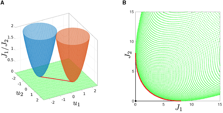
Figure 1. Sketch (red lines) of a Pareto set (A) and Pareto front (B) for min{J(u)|u ∈ ℝ2} with J:ℝ2 → ℝ2, and . The goal is to simultaneously minimize J1 and J2 represented by the blue and the orange paraboloid, respectively.
4.2.1 Problem formulation
Now we turn to our PDE-constrained multiobjective optimization problem (MOP). Given the canonical embedding and two desired states , we consider the following strictly convex MOP:
where σ > 0, 𝔳 ∈ C(Ω; ℝd), 𝔣 ∈ and 𝔶° ∈ H hold. Recall that a unique (weak) solution 𝔶𝔲 ∈ follows from standard results for any control 𝔲 ∈ ; cf., e.g., [38, 39].
Due to convexity it can be proven that a sufficient first-order optimality condition for is given as follows: If there exist a weight satisfying together with an element the conditions
then is a Pareto optimal point for ; see [12] (Theorem 3.27) and [13] (Section 2.1), for instance.
Remark 12. For fixed weight we observe that (17) is a sufficient first-order optimality condition for the (strictly) convex problem
with the choice . This motivates the well-known weighted sum method; cf. [40]. By varying the weight α ∈ [0, 1] the strictly convex problem (18) is solved. This requires many optimization solves, and model order reduction offers the possibility to speed-up the solution process. ◇
For arbitrarily chosen α ∈ [0, 1] we set
Following Remark 12, we consider the (strictly) convex scalar optimization problem
Next, we discretize in space using piecewise linear finite elements (FE). Let m = ny = nu, nz = 2m be valid and φ1, …, φm ∈ V denote the FE ansatz functions. The FE subspace is . For (t, x) ∈ ΩT we approximate the state and control as
respectively. Moreover, let
for (t, x) ∈ Q. Finally, we introduce the m × m matrices
Now problem is approximated by the following FE optimization problem
where fe = L2(0, T; ℝm) and fe = H1(0, T; ℝm). Notice that in this semidiscrete setting, our problem is equivalent to (1a) of Section 3. For (10) we derive
where we have used u(t) = R−1B(t)⊤Wp(t) = p(t)/σ.
In particular, a solution to can be computed by solving the sufficient first-order optimality system (13). For the specific case of we have
with
and .
In conclusion, to compute the Pareto front of the multiobjective optimization problem with a weighted sum approach we have to solve several optimality systems of the form (20) with changing parameter α. For the gramian based MOR approach we proceed as described in Algorithm 1.
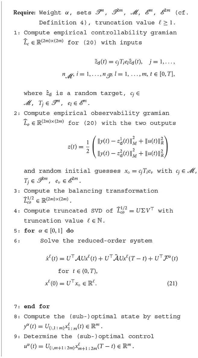
Algorithm 1. Gramian-based MOP using the weighted sum approach.
Remark 13.(1) Steps 1–4 of Algorithm 1 we call training or offline phase. For the gramian orthogonal matrices set 2m, respectively the positive constant set we choose n = n = 3, where and 1 ∈ . The other two orthogonal matrices and scalars were chosen randomly. Furthermore, we restrict the set 2m to ten random unit vectors to save computational effort. Altogether, we compute 3 × 3 × 10 = 90 trajectories to (20) to get the empirical controllability gramian. For ẑd we choose a random input instead of δ-impulse inputs; cf., e.g., [26].
(2) Note that our gramian-based approach ensures sufficiently good approximation qualities for varying desired state for α ∈ [0, 1]. This is required in the weighted sum method.
(3) For solving the dynamical systems (20) and (21) over a fixed time horizon [0, T] we use the implicit Euler scheme with the equidistant time grid tj = (j − 1)Δt and Δt = T/(n − 1) for j = 1, …, n with step size Δt > 0. One can show that the resulting linear system is uniquely solvable.
(4) Since the empirical gramians are trained with respect to the desired state, the resulting basis functions are flexible while using different targets. Therefore, they are also more robust for a varying parameter α, which is pretty important while computing the Pareto front. ◇
In our numerical experiments we compare the results that we got from Algorithm 1 with the ones obtained from a POD reduced-order modeling approach. The snapshots used to generate the POD basis are the solutions of (20) while computing the controllabilty and observability gramians in Algorithm 1. Clearly, this is done only for fair comparison purposes among the techniques. In general, building a POD model capable of approximating the solution of problems with different targets would require to run many simulations varying targets and controls. Unfortunately this is possible only if the targets are known a-priori. Otherwise the only option remaining is choosing random quantities, which would require exactly the same effort of the gramian approach. As we can see, the big difference is that the gramian approach is capable to exploit the randomness to construct a good approximation of the full order model, while the POD seriously struggles if the generated snapshots are not close to the optimal solution of the problem. Furthermore, notice that if we train our POD model by computing snapshots for varying targets and controls we would get a huge amount of snapshots, which will lead to a costly SVD, while the gramian have the advantage to lead to perform SVDs on matrix which have the same size of the problem. The costly SVD for the POD model is directly noticeable at the CPU time of the offline phase; cf. Table 2.
4.2.2 Numerical results
In the following numerical test the chosen parameter and problem required functions are summarized in Table 1.
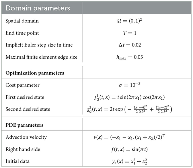
Table 1. Domain, optimization and PDE data for the numerical implementation of .
First of all, already in Figure 2 one can notice the better accuracy of the proposed approach based on empirical gramians for two different number of reduced order models. To better quantify the accuracy of the reduced-order solutions we compare the absolute errors
and also the relative errors
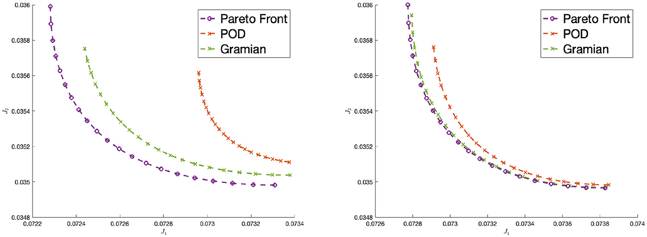
Figure 2. Pareto front for the full-order model, for the empirical gramian-based model and the classical POD model with ℓ = 30 (left plot) and ℓ = 50 (right plot) basis functions.
These errors are reported in Figure 3 for the gramian and POD approaches. As one can see, the empirical gramians perform better than the POD method. Since the desired states and are not part of the training set, it is way harder for the POD-based reduced order model to reconstruct the optimal solution. Also switching the desired states and afterwards one get similar approximation results. This shows the advantage of flexibility of the gramian-based approach. With significant reduction of time (due to cheaper SVDs), one can prepare a basis which is more suitable for varying targets and thus different optimal control problem. This is a large advantage if one considers that often the POD basis must be tailored for each problem at a time. In Table 2, one can see the significant speed-up of the offline phase with the empirical gramians method with respect to the POD one. We picked here the cases ℓ = 30 and ℓ = 50. As said, for the gramian approach we can add all snapshots up in two matrices, whose sizes coincide with the dimension of the problem. For the POD basis, instead, we need a way larger matrix, which depends on the number of snapshots. If one generates many snapshots, as in this case, the SVD of such a matrix gets numerical costly. The reason is that for multiple snapshots the matrix that has to be decomposed by SVD gets larger; cf. [11] (Remark 2.12).
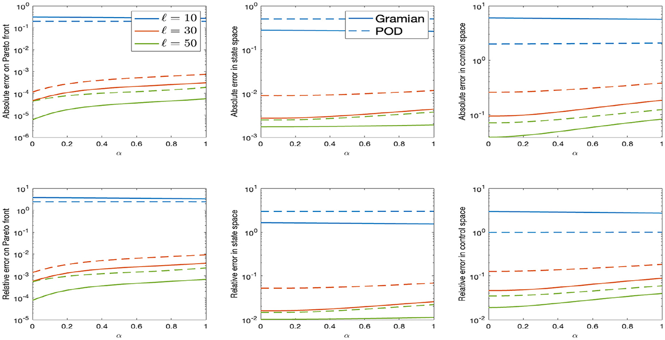
Figure 3. Errors for the reduced order solutions with empirical gramians (solid line) compared to POD approximimation (dashed line). The parameter ℓ represents the number of basis functions.
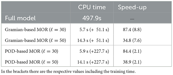
Table 2. CPU times to solve the multiobjective optimization problem and corresponding speed-ups for the respective MOR techniques for ℓ basis functions.
In the brackets there are the respective values including the training time. Notice that the offline time for the gramian-based MOR is significantly lower than for the POD method which leeds to better speed-up factors. The reason for this is that the required SVD for the POD basis computation has to be computed for a much larger data matrix including all snapshots.
4.3 Model predictive control
In the second example we show the potential of the empirical gramians in a model predictive control (MPC) framework. MPC is an optimization based method for the feedback control of dynamical systems where the time horizon usually tends to infinity; see, e.g., [14] for a general introduction and [41] for parabolic PDEs. For large terminal time T we are considering problems of the form
MPC is based on iterative, finite-horizon optimization of dynamical control problems. Let first fix a time discretization with initial time step t0 and tk = t0 + kΔt for Δt > 0 and k ∈ ℕ. Fixed a time shift Tpred = NΔt for N > 0, N ∈ ℕ, we compute an optimal control uk such that uk(ti) is minimizing the cost function for ti in the discrete time interval [tk, tk + Tpred], i.e., i = k, …, k + N. Now, only the optimal control over the discrete time interval [tk, tk + Tf] (Tf = MΔt with 0 < M ≤ N) is stored and the previous procedure is repeated starting from the new resulting current state at time tk + Tf. This yields to a new optimal control uk+1 which will contribute to another piece of the final reconstructed suboptimal control for the whole infinite horizon. In conclusion we are solving iteratively optimal control problems, where the finite prediction horizon keeps being shifted forward. The parameter Tpred is called MPC prediction horizon and Tf is the MPC feedback time step. The reason why we are building a feedback control relies on the fact that each new computed optimal control for a given time window depends on the current state of the system. We present our MPC method in Algorithm 2.
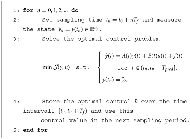
Algorithm 2. Model predictive control (MPC).
4.3.1 Problem formulation
In our numerical example we study the following problem:
where the spaces , and , the linear embedding operator and the data σ, 𝔶°, 𝔳 and 𝔣 have been introduced at the beginning of Sections 4, 4.2.1. Moreover, let α ∈ L∞(0, T) be scalar-valued parameter function andχω the characteristic function of a nonzero subset ω ⊂ Ω. Recall that a unique (weak) solution 𝔶𝔲 ∈ for any control 𝔲 ∈ follows from standard results; see, e.g., [38, 39].
Next, we proceed analog to Section 4.2 to derive the semidiscrete problem with weighted norms. The semidiscrete first-order necessary and sufficient optimality system of is equivalent to solving the system
for x = (y, q), q(t) = p(T − t), with y and p solution of state and adjoint equation of respectively, and
Moreover, we have u(t) = M−1B⊤p(t)/σ.
Now, the possible approach for applying model-order reduction to would be to apply the POD method; cf., e.g., [11]. One would run simulations of state and adjoint equations varying the control u in order to construct a POD basis. The more the inputs u for the training are closer to the unknown optimal control, the better the POD approximation will be. Clearly this shows the limitation of this approach, since it is not really possible to guess a-priorly what the optimal control will be. Anyway, since we are in an MPC framework, one could think of paying the price of solving occasionally FE models to generate (and update) the POD basis and perform the rest of the runs with the resulting reduced-order model. This strategy has also the advantage that can be controlled by the use of an a-posteriori error estimator to decide when trigger the update. For this MPC-POD method we refer to [15, 42]. With respect to this method, the gramian-based approach offers additional advantages:
1) The possibility of training the controllability gramian (and thus the reduced-order model) choosing as input the advection coefficient α(t). In such a way, the resulting basis functions will be less sensitive to perturbations of this advection coefficient.
2) Similarly, we can train the observability gramian by choosing as output z(t) = M−1B⊤p(t)/σ, which nothing else that the first-order optimality condition of the perturbed optimal control problem that has (22) as optimality system. In such a way, the reduced-order model will be capable to reconstruct the optimal control with high accuracy.
As also pointed out in [15], in fact, the MPC-POD method suffers in presence of advection already for a small Peclet number and any strong deviation from the original POD snapshots can also lead to inaccuracy. Although the a-posteriori error estimator mitigates these problems, the continue triggering of the update of the basis has also a negative impact in the overall time performances of the algorithm. The gramian based MPC can overcome this by preparing a reduced-order model slightly sensible to perturbations of advection and optimal control. The basis functions are capable to keep track of the changes in this case, thanks to the randomized training performed at the begin. For a more detailed description of the gramian based MPC we refer to Algorithm 3, for the MPC-POD algorithm we refer to [15] (Algorithm 11).
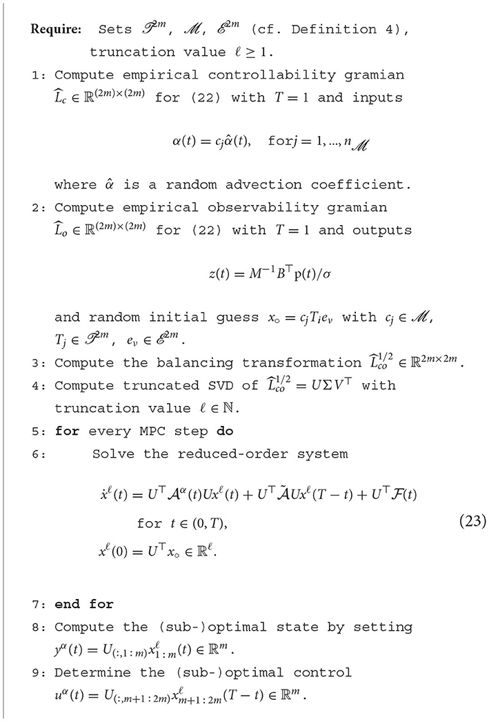
Algorithm 3. Gramian-based MPC.
4.3.2 Numerical results
For the following numerical tests we choose the same domain and PDE parameter than in Section 4.1.1 apart from the end time point, which is here set to T = 250. The additional advection coefficient function α ∈ L∞(0, T; ℝ) is chosen randomly in a specified range, which will be varied to defined different test cases. We report the other chosen parameters in Table 3.
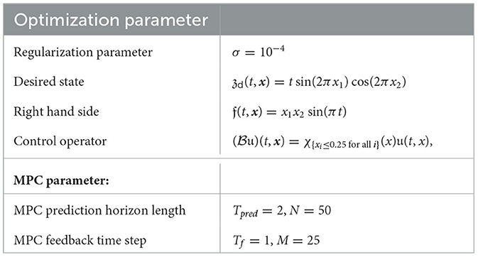
Table 3. Optimization and MPC data for the numerical implementation of .
The numerical results are reported in Tables 4, 5. The quantity , , and are the absolute errors and the relative errors in approximating full-order optimal state ȳ and control ū, respectively. More precisely, being ȳℓ and ūℓ a reduced-order model solution, we define
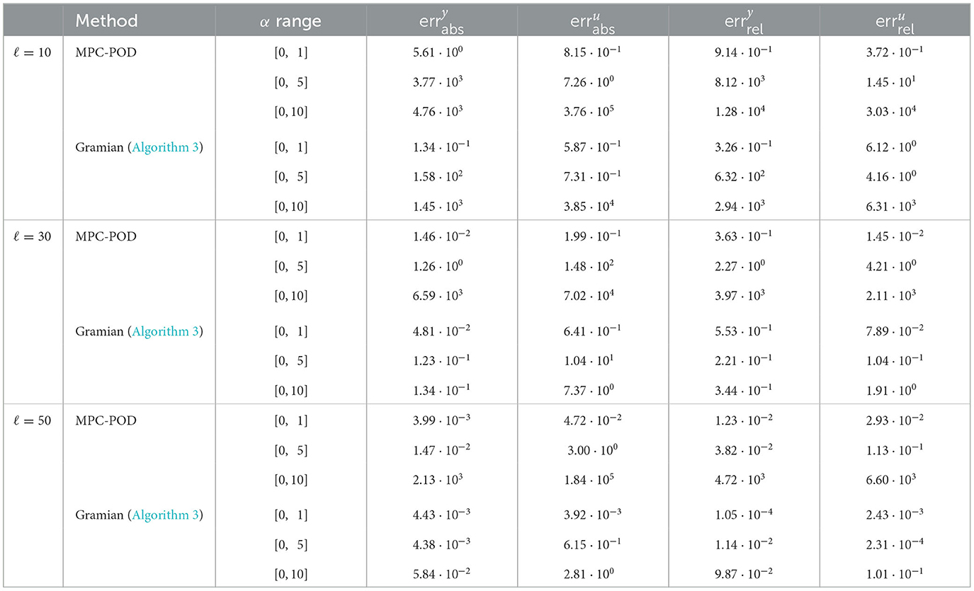
Table 4. Error in approximating the optimal state ȳ and control ū solution of the discretized full order model with randomly chosen advection coefficient function α in the reported range and ℓ ∈ {10, 30, 50} basis functions.
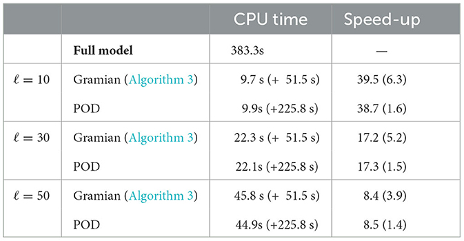
Table 5. Average CPU times to solve the MPC framework for and corresponding speed-ups for the respective MOR techniques after 1,000 simulations with randomly chosen advection coefficients function α.
where the time integrals are realized numerical by applying a standard trapezoidal approximation. As said, since we train the gramians with respect to the advection coefficient α, we obtain basis functions which are robust with respect to changes of the advection term. This can be seen in Table 4, where the relative error increases significantly only for the largest range of [0, 10].
The MPC-POD method, instead, starts loosing accuracy already at the stage [0, 5]. Furthermore, the relative error for the control resulting from Algorithm 3 is from two to four order of magnitude smaller with respect to the MPC-POD one. In particular, in the last case of α(t) ∈ [0, 10] the MPC-POD method is not practically usable. Therefore, we can say that Algorithm 3 is able to recover the optimal solution with a better approximation than the MPC-POD method. Let us mention, that for a fair comparison, we used the same snapshots for the two approaches. The problem for POD is that the resulting basis has no capability to track the information carried by perturbing the advection, while the gramian can. Anyway, the deterioration of accuracy for increasing advection emerges also in the context of the gramian basis, although does not affect its usability in our numerical tests. From Table 5, one can also see another disadvantage of the POD method.
Since we are using the same number of snapshots for the two techniques, the POD matrix has the dimension of Nx × L, where Nx is the of FE nodes and L the number of snapshots. Clearly, if L ≫ Nx, the time to compute a POD basis, i.e., performing a SVD on the matrix Nx × L is significantly larger than the two SVDs required for the Nx × Nx gramians. This reflects the difference on the overall time speed-up between MPC-POD (1.7) and Algorithm 3 (4.8). We can then conclude that our proposed gramian based approach has the double advantage of robustness with respect to variation of the advection field and overall time speed-up in comparison to the MPC-POD method.
4.3.3 A-Posteriori error analysis
To validate our numerical approach we control the MOR error by an a-posteriori error estimate. The idea is that the error of the difference between the (unknown) optimal control and its suboptimal approximation computed by the MOR-based discretization can be estimated without knowing the optimal solution (𝔶α, 𝔲α) to . The techniques are based on well-known Galerkin-type estimates. In the Appendix we have summarized the results. For more details we refer to [8, 10, 11], for instance.
From Figure 4 it can be seen that in each step of the MPC algorithm the error in the computed suboptimal controls are smaller than 0.1. The impact of the truncation value ℓ on the error is thoroughly examined in [43].
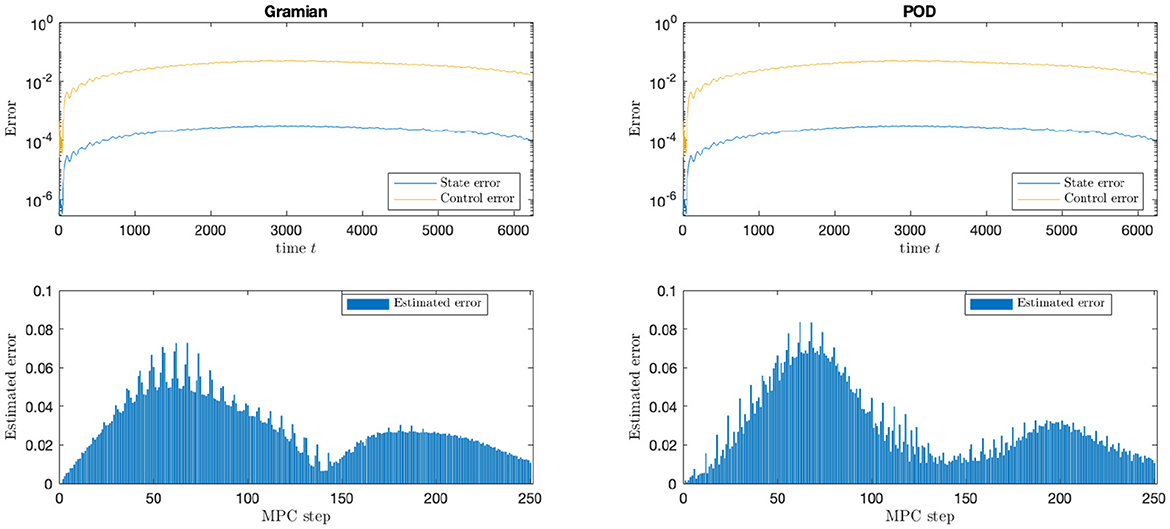
Figure 4. Reduced MPC with one reduced gramain (left) and POD (right) basis with reduced basis rank ℓ = 50 and range(α) = [0.1]. One every column are the absolute L2-spatial-difference in state and control over the time, i.e., and (top) and the particular error estimates for every MPC step.
5 Conclusions
In the present paper empirical gramian have been used to derive reduced order models tailored for the first-order optimality system which consists of the coupled state and dual equation. Here, data of the optimization problem serve as inputs for the computation of the gramian matrices. The validation by a-posteriori error analysis shows that we get reliable reduced order models which turn out to perform better than reduced order models based on a standard POD, which utilizes exactly the same snapshots for the ROM. The reason of such performances is the possibility of including controllability and observability knowledge through the empirical gramian approach. This leads to the fact that the gramian-based ROM is more appropriate for the optimization purposes. Finally, as future perspective, the proposed approach can be applied to nonlinear dynamical systems as well. Here, the accuracy could be checked by hierarchical a-posteriori error analysis; see, e.g., [44], which extends the work in [45]. To get an efficient numerical reduced order realization for the nonlinear dynamical system, one would need to apply the (discrete) empirical interpolation method (cf. [22–24]) or missing point evaluation (cf. [25]).
Data availability statement
The original contributions presented in the study are included in the article/Supplementary material, further inquiries can be directed to the corresponding author.
Author contributions
All authors listed have made a substantial, direct, and intellectual contribution to the work and approved it for publication.
Funding
The authors acknowledge funding by the Independent Research Grant Efficient model order reduction for model predictive control of non-linear input-output dynamical systems of the Zukunftskolleg at the University of Konstanz and by the Deutsche Forschungsgemeinschaft (DFG) for the project Localized Reduced Basis Methods for PDE-Constrained Parameter Optimization under contract VO 1658/6-1.
Conflict of interest
The authors declare that the research was conducted in the absence of any commercial or financial relationships that could be construed as a potential conflict of interest.
Publisher's note
All claims expressed in this article are solely those of the authors and do not necessarily represent those of their affiliated organizations, or those of the publisher, the editors and the reviewers. Any product that may be evaluated in this article, or claim that may be made by its manufacturer, is not guaranteed or endorsed by the publisher.
Supplementary material
The Supplementary Material for this article can be found online at: https://www.frontiersin.org/articles/10.3389/fams.2023.1144142/full#supplementary-material
References
1. Becker R, Kapp H, Rannacher R. Adaptive finite element methods for optimal control of partial differential equations: basic concept. SIAM J Control Optimiz. (2000) 39:113–32. doi: 10.1137/S0363012999351097
2. Liu W, Yan N. A posteriori error estimates for distributed convex optimal control problems. Adv Comp Math. (2001) 15:285–309. doi: 10.1023/A:1014239012739
3. Holmes P, Lumley J, Berkooz G, Rowley C. Turbulence, Coherent Structures, Dynamical Systems and Symmetry. 2nd ed. Cambridge: Cambridge University Press (2013).
4. Hesthaven J, Rozza G, Stamm B. Certified Reduced Basis Methods for Parametrized Partial Differential Equations. SpringerBriefs in Mathematics. Cham: Springer (2016).
5. Quarteroni A, Manzoni A, Negri F. Reduced Basis Methods for Partial Differential Equations: An Introduction. UNITEXT-La Matematica per il 3+2. Cham: Springer (2016).
6. Benner P, Ohlberger M, Cohen A, Willcox K. Model Reduction and Approximation. Philadelphia, PA: Society for Industrial and Applied Mathematics (2017).
7. Benner P, Mehrmann V, Sorensen D. Dimension reduction of large-scale systems: Proceedings of a Workshop held in Oberwolfach, Germany, October 19–25, 2003. In: Lecture Notes in Computational Science and Engineering. Heidelberg: Springer (2006).
8. Hinze M, Volkwein S. Error estimates for abstract linear-quadratic optimal control problems using proper orthogonal decomposition. Comput Optim Appl. (2008) 39:319–45. doi: 10.1007/s10589-007-9058-4
9. Antoulas AC. Approximation of Large-Scale Dynamical Systems. Advances in Design and Control. Philadelphia, PA: SIAM (2009).
10. Tröltzsch F, Volkwein S. Pod a-posteriori error estimates for linear-quadratic optimal control problems. Comput Optim Appl. (2009) 44:83–115. doi: 10.1007/s10589-008-9224-3
11. Gubisch M, Volkwein S. Proper Orthogonal Decomposition for Linear-Quadratic Optimal Control, Chapter 1. Philadelphia, PA: SIAM (2017). p. 3–63.
13. Banholzer S. ROM-Based Multiobjective Optimization with PDE Constraints (Ph.D. thesis). University of Konstanz (2021). Available online at: http://nbnresolving.de/urn:nbn:de:bsz:352-2-1g98y1ic7inp29 (accessed November 28, 2023).
14. Grüune L, Pannek J. Nonlinear Model Predictive Control: Theory and Algorithms. 2nd ed. London: Springer (2016).
15. Mechelli L. POD-based State-Constrained Economic Model Predictive Control of Convection-Diffusion Phenomena (Ph.D. thesis), University of Konstanz (2019). Available online at: http://nbn-resolving.de/urn:nbn:de:bsz:352-2-2zoi8n9sxknm1 (accessed November 28, 2023).
16. Bellman R. Introduction to the Mathematical Theory of Control Processes. Vol. II: Nonlinear Processes. New York, NY: Academic Press (1971).
17. Isidori A. Nonlinear Control Systems: An Introduction. 2nd ed. Berlin; Heidelberg: Springer-Verlag (1989).
18. Zhou K, Doyle J, Glover K. Robust and Optimal Control. Upper Saddle River, NJ: Prentice-Hall (1996).
19. Hernández-Lerma O, Laura-Guarachi L, Mendoza-Palacios S, González-Sánchez D. An Introduction to Optimal Control Theory. The Dynamic Programming Approach. Texts in Applied Mathematics. Cham: Springer (2023).
20. Lall S, Marsden JE, Glavaški S. Empirical model reduction of controlled nonlinear systems. In: IFAC Proceedings Volumes, 32:2598–2603. 14th IFAC World Congress 1999, Beijing, Chia, 5–9 July. Oxford: Pergamon (1999).
21. Garcia J, Basilio J. Computation of reduced-order models of multivariable systems by balanced truncation. Int J Syst Sci. (2002) 33:847–54. doi: 10.1080/0020772021000017308
22. Barrault M, Maday Y, Nguyen N, Patera A. An empirical interpolation method: application to efficient reduced-basis discretization of partial differential equations. Comp Rendus Math. (2004) 339:667–72. doi: 10.1016/j.crma.2004.08.006
23. Chaturantabut S, Sorensen D. Nonlinear model reduction via discrete empirical interpolation. SIAM J Sci Comp. (2010) 32:2737–64. doi: 10.1137/090766498
24. Chaturantabut S, Sorensen D. A state space estimate for POD-DEIM nonlinear model reduction. SIAM J Numer Anal. (2012) 50:46–63. doi: 10.1137/110822724
25. Astrid P, Weiland S, Willcox K, Backx T. Missing point estimation in models described by proper orthogonal decomposition. IEEE Trans Automat Contr. (2008) 53:2237–51. doi: 10.1109/TAC.2008.2006102
27. Kalman R. Mathematical description of linear dynamical systems. SIAM J. Control Optim. (1963) 1:182–92. doi: 10.1137/0301010
29. Baur U, Benner P. Cross-gramian based model reduction for datasparse systems. Electron Transact Numer Anal. (2008) 31:256–70. doi: 10.1137/070711578
30. Moore B. Principal component analysis in linear systems: controllability, observability, and model reduction. IEEE Trans Automat Contr. (1981) 26:17–32. doi: 10.1109/TAC.1981.1102568
31. Aldhaheri R. Model order reduction via real schur-formdecomposition. Int J Control. (1991) 53:709–16. doi: 10.1080/00207179108953642
32. Gallivan K, Vandendorpe A, Van Dooren P. Sylvester equations and projection-based model reduction. J Comput Appl Math. (2004) 162:213–29. doi: 10.1016/j.cam.2003.08.026
33. Sorensen D, Antoulas A. The sylvester equation and approximate balanced reduction. Linear Algebra Appl. (2002) 351/2:671–700. doi: 10.1016/S0024-3795(02)00283-5
34. Betts JT. Practical methods for optimal control and estimation using nonlinear programming. In: Advances in Design and Control. 2nd, ed. Philadelphia, PA: SIAM (2010).
35. Villanueva M, Jones C, Houska B. Towards global optimal control via koopman lifts. Automatica. (2021) 132:109610. doi: 10.1016/j.automatica.2021.109610
36. Evans L. Partial Differential Equations. Graduate Studies in Mathematics. American Mathematical Society. Providence, RI: American Mathematical Society (2010).
37. Kunisch K, Volkwein S. Galerkin proper orthogonal decomposition methods for parabolic problems. Numer Math. (2001) 90:117–48. doi: 10.1007/s002110100282
38. Dautray R, Lions J-L. Mathematical Analysis and Numerical Methods for Science and Technology. Vol. 5: Evolution Problems I. Berlin: Springer (2000).
39. Pazy A. Semigoups of Linear Operators and Applications to Partial Differential Equation. Berlin: Springer (1983).
40. Zadeh L. Optimality and non-scalar-valued performance criteria. IEEE Trans Automat Contr. (1963) 8:59–60. doi: 10.1109/TAC.1963.1105511
41. Azmi B, Kunisch K. A hybrid finite-dimensional rhc for stabilization of time-varying parabolic equations. SIAM J Control Optimiz. (2019) 57:3496–526. doi: 10.1137/19M1239787
42. Mechelli L, Volkwein S. POD-based economic model predictive control for heat-convection phenomena. In: Radu FA, Kumar K, Berre I, Nordbotten JM, Pop IS, , editors. Numerical Mathematics and Advanced Applications ENUMATH 2017. Cham: Springer International Publishing (2019). p. 663–671.
43. Rohleff J. Data-Driven Model-Order Reduction for Model Predictive Control (Master thesis). University of Konstanz (2023).
44. Azmi B, Petrocchi A, Volkwein S. Adaptive parameter optimization for an elliptic-parabolic system using the reduced-basis method with hierarchical a-posteriori error analysis. arXiv. (2023)
Keywords: model order reduction, empirical gramians, proper orthogonal decomposition, parabolic partial differential equations, multiobjective optimization, model predictive control, a-posteriori error analysis
Citation: Mechelli L, Rohleff J and Volkwein S (2023) Model order reduction for optimality systems through empirical gramians. Front. Appl. Math. Stat. 9:1144142. doi: 10.3389/fams.2023.1144142
Received: 13 January 2023; Accepted: 14 November 2023;
Published: 11 December 2023.
Edited by:
Jan Heiland, Max Planck Society, GermanyReviewed by:
Abdulsattar Abdullah Hamad, University of Samarra, IraqZhihua Xiao, Yangtze University, China
Copyright © 2023 Mechelli, Rohleff and Volkwein. This is an open-access article distributed under the terms of the Creative Commons Attribution License (CC BY). The use, distribution or reproduction in other forums is permitted, provided the original author(s) and the copyright owner(s) are credited and that the original publication in this journal is cited, in accordance with accepted academic practice. No use, distribution or reproduction is permitted which does not comply with these terms.
*Correspondence: Stefan Volkwein, U3RlZmFuLlZvbGt3ZWluQHVuaS1rb25zdGFuei5kZQ==
†These authors have contributed equally to this work and share first authorship