 Mohammadamin Sedghizadeh
 Matthew van den Berghe
 Robert Shcherbakov
95% of researchers rate our articles as excellent or good
Learn more about the work of our research integrity team to safeguard the quality of each article we publish.
Find out more
ORIGINAL RESEARCH article
Front. Appl. Math. Stat. , 30 March 2023
Sec. Statistical and Computational Physics
Volume 9 - 2023 | https://doi.org/10.3389/fams.2023.1126952
This article is part of the Research Topic Physical and Statistical Approaches to Earthquake Modeling and Forecasting View all 5 articles
Microseismicity is expected in potash mining due to the associated rock-mass response. This phenomenon is known, but not fully understood. To assess the safety and efficiency of mining operations, producers must quantitatively discern between normal and abnormal seismic activity. In this work, statistical aspects and clustering of microseismicity from a Saskatchewan, Canada, potash mine are analyzed and quantified. Specifically, the frequency-magnitude statistics display a rich behavior that deviates from the standard Gutenberg-Richter scaling for small magnitudes. To model the magnitude distribution, we consider two additional models, i.e., the tapered Pareto distribution and a mixture of the tapered Pareto and Pareto distributions to fit the bi-modal catalog data. To study the clustering aspects of the observed microseismicity, the nearest-neighbor distance (NND) method is applied. This allowed the identification of potential cluster characteristics in time, space, and magnitude domains. The implemented modeling approaches and obtained results will be used to further advance strategies and protocols for the safe and efficient operation of potash mines.
Mining is typically accompanied by various degrees of seismic activity. This is known as mining-induced seismicity and it is observed both in hard rock and soft rock environments [1–4]. The mining seismicity is typically induced by different operations, such as rock excavation, rock blasting, and others. This is a direct result of a constantly changing underground stress field that leads to the creation of new fracture zones or reactivation of existing fractures/faults [3–5]. Induced seismicity is one of the hazards in mines and it is observed in potash, coal, metal ore, uranium, and diamond mines within a wide range of geological settings [6–8]. Induced seismicity is observed during other anthropogenic operations such as: hydrocarbon production from tight shale reservoirs, enhanced geothermal energy generation, and high-volume underground fluid injection [9–11].
In the context of mining industry, several geohazards are associated with mining operations. These include: water inflow, the occurrence of earthquakes, rockbursts, development of fracture zones, to mention a few [2, 4, 12, 13]. In case of potash mines, the intrusion of undersaturated brine into a mine has the potential to inflict significant damage to a mine internal structure and result in erosion of pillars, weakening of openings, and rupture of the caprock [12–14]. Among those geohazards, the occurrence of earthquakes and /or microseismicity is a critical factor that has to be monitored and studied. The occurrence of mining seismicity is controlled by various aspects of mine operations and settings such as depth, spatial expanse, geological setting, which includes varied rock formations and layering, the presence of fault systems and fractures, as well as the changes in the ambient stress field and pore pressure [15]. In hard rock mines, seismicity is usually associated with an active mining front due to rock excavation [16]. Whereas in soft rock mining, the host rocks may experience plastic creep due to rock extraction. As a result, the seismicity can be observed in the surrounding rocks [17]. Various aspects of the microseismicity has been also extensively studied in rock fracture experiments, for example in Refs. [18–20].
In this study, we focused on the statistical analysis of microseismicity associated with mining operations in a Saskatchewan, Canada, potash mine. Several statistical models have been considered to investigate various aspects of induced seismicity in the mine. Specifically, a comprehensive analysis of the frequency-magnitude statistics of the mining events has been performed. This included the estimation of the magnitude of the completeness of the analyzed catalog by utilizing several catalog-based methods. Also, we modeled the frequency-magnitude statistics of microseismicity by considering several parametric distributions to establish the most appropriate model that was relevant to that mine. In addition, we also considered the standard exponential distribution, the upper-truncated and tapered Pareto distributions, and the mixture of the above distributions. The maximum likelihood method was utilized to estimate the model parameters. In order to classify the mining seismicity in terms of the mode of triggering and possible rheological regimes, the NND clustering method was applied. The influence of the mining operations on the triggering of microseismicity was quantified by using the cross-correlation analysis. The main goal of this work was to establish and quantify the current pattern of seismic activity in the mine in order to monitor and observe any significant deviations in seismic activity during the future mine operation. The studied seismic catalog also presented a unique opportunity to investigate the statistical properties of microseismicity in the soft rock environment.
Potash deposits in Saskatchewan are mined from the Prairie Evaporite formation. This layer contains one of the largest global potash deposits of sylvinite ore and is mainly used for fertilizer production. Saskatchewan potash deposits are unique in the world because they are very extensive, flat, and generally intact, leading to low-cost extraction. Evidence suggests that the age of these strata of sediments is Middle Devonian. The Prairie Evaporite formation, with a thickness of 100–200 m, is located below 400–500 m of Devonian carbonate with thin layers of shales, anhydrite, and salts followed by 400–500 m of Cretaceous shale and sands with glacial tills on top [21–23]. Besides common microseismicity, several moderate earthquakes have been observed in the past in Saskatchewan's potash mines [12, 13]. Those earthquakes are thought to occur in the layers above the mining horizon, mainly in the carbonate Dawson Bay formation. Changes in the local stress regime and ongoing convergence of the underlying strata into the openings are commonly viewed as one of the leading causes of mining-induced seismicity in potash mines in Saskatchewan [24].
To safely operate a mine, it is important to impose reasonable control on the factors that can trigger earthquakes [3, 4, 25, 26]. In this respect, the statistical analysis of past mining seismicity plays a critical role [27, 28]. By analyzing the patterns of seismicity, one can infer more about their possible causes and relate them to specific mining operations or geomechanical processes. As a result, this can help mitigate the risk associated with induced mining seismicity. The standard approach involves the analysis of the frequency-magnitude statistics and spatio-temporal patterns of mining seismicity [27, 29–31]. This is used to improve the re-entry protocols in mines [32, 33], to study aftershocks and clustering [28, 34], to develop the hazard assessment approaches of mining seismicity [2, 31]. In addition, one can also consider more advanced methods to study mining seismicity. These include the analysis of the clustering aspects of seismicity; any possible deviations from Poisson statistics in the occurrence of events; whether earthquake magnitudes are correlated or not. Therefore, the statistical analysis is a crucial step in assessing the associated seismic hazard and is used to mitigate the corresponding risk.
The statistical analysis of seismicity offers various approaches to quantify the occurrence of earthquakes in magnitude and spatio/temporal domains. Among those approaches, the clustering aspects of seismicity can be used to identify possible triggering mechanisms that drive the occurrence of earthquakes. Various clustering identification methods have been developed in the context of the statistical data analysis [35, 36] and several have been used to study the spatio-temporal patterns of natural and mining seismicity [37, 38]. The overview of clustering aspects of microseismicity in Australian and Canadian mines was provided by Hudyma [39]. It was suggested that mining seismicity is primarily induced by the local failure of rock mass due to various factors including: mining-induced stresses, geological structures, and mining operations. That analysis was based on the application of the hierarchical agglomerative clustering methods to identify individual seismic sources and rock mass failure mechanisms [39]. The mean minimum distance, hierarchical, and K-means clustering methods were used in the study of seismicity in a coal mine in Poland [40]. A 3D spatial clustering methodology for short-term mining seismicity was developed [41] by introducing modifications to the density-based clustering of applications with noise method [42]. The expectation-maximization algorithm was used to identify probabilistic kernels associated with active fault segments to classify seismic events based on their seismic source mechanism, location, and its uncertainty [43]. A hierarchical clustering analysis incorporating Ward's minimum variance method was applied to seismicity in a coal mine to quantify the seismic hazard [44]. One of the goals of the clustering analysis is to identify the relationship between seismic sources and the influence of inducing operations in order to assess and quantify the seismic hazard. For example, the effect of declustering of earthquake catalogs on the frequency-magnitude analysis of seismicity was investigated to asses the estimation of the b-value [45].
A separate method to analyze the clustering of seismicity is based on the assumption that earthquakes can be linked by a suitably computed nearest-neighbor distance in a multidimensional space spanned by the time, space, and magnitude domains. It is known as the nearest-neighbor distance (NND) method and it was first proposed by Baiesi and Paczuski [46] and considerably expanded by Zaliapin et al. [47], Zaliapin and Ben-Zion [48, 49]. It was also adapted to perform declustering of earthquake catalogs [50]. The NND method was also applied to analyze the seismicity in the Western Canada Sedimentary Basin due to a significant increase in induced seismicity observed in the last decade [51–53].
The paper is organized as follows: Section 2 presents the background information about the mine and seismicity catalog. In Section 3 the statistical methods to analyze mining seismicity are formulated. The results of the statistical analysis are reported in Section 4. Section 5 discusses the results and conclusions are drawn in Section 6.
In order to analyze the induced microseismicity in a potash mine in Saskatchewan, a manually reviewed microseismic catalog was used. The spatial distribution of microseismic events above magnitude m ≥ −2.97 is shown in Figure 1. The catalog spans the time interval between 01/05/2019 and 07/09/2021. The original catalog contained 11,633 events. For the analysis, it was reduced to 9,268 events by manually removing the events associated with the network calibrating surface shots that were performed between 02/12/2021 and 02/19/2021. The magnitudes of events in the catalog are reported with two decimal points.
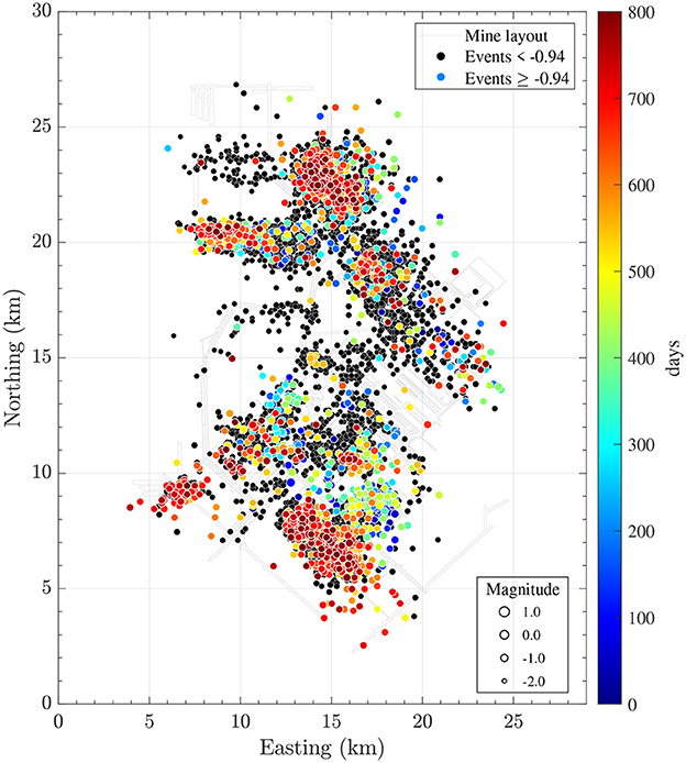
Figure 1. The plot of the epicenters of microseismicity in a potash mine in Saskatchewan, Canada. The events were recorded from May 1, 2019, to July 9, 2021. The colored solid circles represent events with magnitudes above m ≥ −0.94. Different colors indicate the time of the occurrence of events and are given by the color bar with the corresponding times in days starting from May 1, 2019. All other events between magnitudes −2.97 ≤ m < −0.94 are shown as black solid circles. The light gray lines illustrate the layout of the mine which includes the mine shafts and tunnels.
To perform the statistical analysis of mining seismicity, we analyze several aspects of the occurrence of events. This was accomplished by performing the analysis of event catalog data in magnitude, temporal, and spatial domains. The following specific methods were employed.
In statistical modeling of seismicity, the occurrence of seismic events can be approximated as a stochastic marked point process in time and space. In the simplest case, it is assumed that the event magnitudes are not correlated and the occurrence of events is fully controlled by the rate. This constitutes the Poisson assumption and is commonly used in statistical seismology. If the seismicity rate is constant, the distribution of the interevent times between successive events must follow an exponential distribution with the probability density function:
where λ is a constant seismicity rate and the interevent time Δti = ti − ti−1 defines the time interval between two consecutive events. When the rate is no longer constant λ = λ(t), the distribution of interevent times deviates from the exponential [54].
It was also reported that for some earthquake sequences the distribution of interevent times can be described by the gamma distribution [54, 55]:
where κ > 0 is a shape parameter and θ > 0 is a scale parameter. This is typically associated with the presence of aftershock sequences that decay according to the Omori-Utsu law [56].
The most accepted empirical relationship that describes the distribution of earthquake magnitudes was suggested by Gutenberg and Richter [57]. It gives the cumulative number of events, N(m ≥), above magnitude m:
where b-value is a slope of the fitted line in a semi-logarithmic scale. a is the intercept of this line at magnitude zero and is related to the cumulative number of events above magnitude zero, N(m ≥ 0) = 10a, during a specified time interval. From the statistical point of view, it is more appropriate to separate the distribution of magnitudes and the occurrence rate. The distribution of the magnitudes can be described by the left-truncated exponential distribution [58]:
where f(m) and F(m) are the probability density and cumulative distribution functions, respectively. mmin, is the minimum magnitude cut-off that is above the catalog completeness magnitude mc and β is the model parameter related to the b-value of G-R scaling: β = bln(10). The standard approach to estimate the b-value or parameter β is using the maximum likelihood estimation (MLE). Bender [59] proposed an estimator for β by considering the binning of the earthquake magnitudes. In addition, Tinti and Mulargia [60] developed an approach to estimate the uncertainties of the estimated parameter β for a given confidence interval.
One can also consider more realistic distributions to describe the statistics of event magnitudes. For this, we will use the scalar seismic moment M to characterize the size of an event. It can be computed from the magnitude through an empirical relationship: M = 101.5(m+10.73). The distribution of magnitudes given by Eqs. (4)–(5) becomes a Pareto distribution in the scalar seismic moment domain [61]:
where . The complementary distribution function Φ(M) is related to the cumulative distribution function F(M) = 1 − Φ(M). is the parameter that characterizes the scaling of seismic moments.
From the analysis of the distribution of seismic moments, Kagan [61] suggested using the tapered Pareto distributions as a suitable alternative instead of the original G-R distribution, Equation (3). The probability density function, ftap(M), and complimentary cumulative distribution function, Φtap(M) of the tapered Pareto distribution can be written as follows:
where Mcm is the corner moment, which specifies the magnitude above which the distribution is tapered by the exponential tail. The parameters of the truncated and tapered Pareto distributions can be estimated using the MLE approach [61].
Induced seismicity can exhibit a bimodal structure in its magnitude distributions. To capture this aspect of induced seismicity one can consider a mixture of distributions. This can be achieved by considering the mixture of the tapered Pareto (8) and Pareto (6)distributions:
where w is a mixing weighting factor. The model parameters and weight w can be estimated using the MLE approach.
One of the challenges when performing the statistical analysis of seismicity is the estimation of the magnitude of completeness of a catalog of earthquakes, mc, which is the minimum magnitude above which all events are recorded. This is critical for the parameter estimation of statistical models or analysis of clustering of seismicity as the population must contain events above this threshold to avoid any bias in the obtained results due to missing events. On the other hand, overestimation of mc can result in larger uncertainties in the parameter estimates. To address this issue, the three catalog-based methods most-commonly used to estimate the magnitude of completeness mc were applied: (1) the method of maximum curvature (MAXC) [62]; (2) the G-R b-value stability (MBS) method [63, 64]; and (3) the method based on the goodness-of-fit test (GFT) [62].
In case of MAXC, it was suggested that the completeness magnitude mc can be defined as the magnitude of the bin with the maximum number of events in the histogram of the magnitude distribution [62]. However, this approach tends to underestimate mc, especially in locations characterized by irregular network coverage [65].
In order to estimate mc using the MBS method, Cao and Gao [63] suggested an approach based on the stability of the b-value as a function of the cutoff magnitude, mmin. This method assumes that b-value reaches a plateau when progressively increasing mmin. They define mc as a cutoff magnitude for which the successive changes in b-values are < 0.03. Woessner and Wiemer [64] introduced a modification to this method by defining mc as the magnitude for which the changes in b-value are less than its uncertainty.
In the GFT method, the magnitude of completeness mc, is estimated by comparing the empirical frequency-magnitude distribution with the model that is being used for different cutoff magnitudes [62]. The discrepancy is quantified by computing a goodness-of-fit (gof) value. The cutoff magnitude that achieves the gof above a given percentage level defines mc. In the method, the corresponding model parameters are estimated. The absolute differences in the number of events in each magnitude bin from the observed and the model distribution are used to compute the residuals. This is used to obtain the value of the gof:
where the observed and anticipated cumulative number of occurrences of magnitude in each bin are Ni and Fi, respectively. To normalize the sum, it is divided by the total number of observed events.
The occurrence of seismic events is typically driven by natural or anthropogenic changes in stresses and can also be characterized by interevent triggering. This leads to the formation of seismic sequences with varying degrees of clustering. To study the clustering aspects of natural or induced seismicity one can define a rescaled distance between pairs of events in a hyperspace, which is spanned by the spatial, temporal, and magnitude domains. In this respect, the problem of earthquake classification and clustering is addressed in the works by Baiesi and Paczuski [46], Zaliapin et al. [47], Zaliapin and Ben-Zion [48–50] and is based on minimizing the rescaled relative distance between events and is known as the nearest-neighbor distance (NND) method.
In the NND method, each event i in the catalog is characterized by the time ti, magnitude mi, and hypocenter location (latitude ϕi, longitude λi, and depth di). For each pair of events i and j, one can compute a rescaled distance in spatio-temporal and magnitude domains:
where tij = tj − ti is the time interval between event i and the subsequent event j. The spatial distance rij can be computed as an epicentral distance
where RE = 6, 371 km is the radius of the Earth. The parameter b can be estimated from the G-R relation. df is the fractal dimension of the distribution of the epicenters or hypocenters. It ranges between 1.2 and 1.6 for both local and global earthquake epicenter distributions in 2-dimensional space [66].
The rescaled distance ηij can also be written as a product of rescaled temporal and spatial terms: ηij = TijRij, where
and
For each event j it is possible to find the minimum that defines the nearest-neighbor distance to event j. The corresponding event i that minimizes ηij becomes a parent event for the event j. Therefore, one can compute the distribution of the nearest-neighbor distances η. In addition, it is possible to analyze the distribution of the rescaled times T and rescaled distances R. Finally, one also can compute the joint distribution of (T, R). These distributions can be analyzed to infer any possible modality in the spatio-temporal relationship between events.
When applying the NND analysis and finding the nearest-neighbor distance η for each event, one can obtain a corresponding clustering structure, where events can be classified into groups, by specifying a suitable threshold, ηthresh. This threshold value can be used to separate events into two categories, i.e. clustered and background ones. In addition, there are root events that do not have any parent events. There are events that are both parent and daughter events. And finally, the events that are leaves and are not parents to any events [49].
The cumulative number of events in the catalog starting on May 1, 2019, and ending on July 9, 2021, is plotted in Figure 2 as blue dots. The original catalog contained 11,633 events above magnitude m ≥ −2.97. The events between February 12–19, 2021 were excluded from the analysis as they were mostly initiated by the controlled blasts. The reduced catalog containing 9,268 events was utilized for further analysis in this study and the corresponding cumulative numbers are plotted as brown dots in Figure 2. In addition, the cumulative numbers are plotted for the events above the completeness magnitude mc = −0.94 as yellow dots.
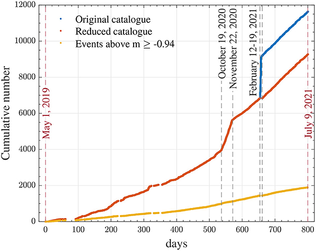
Figure 2. The cumulative number of events of the mining microseismicity during the study time interval from 05/01/2019 until 07/09/2021. The numbers are plotted as: blue solid symbols for the original full catalog with the events above magnitude m ≥ −2.97; red symbols using the reduced catalog, where events associated with the controlled blasts during 12–19/02/2021 were removed; yellow symbols using the reduced catalog for the events above magnitude m ≥ −0.94.
The reduced catalog, given in Figure 2 as brown dots, was analyzed to estimate the magnitude of completeness mc. This was done by using the MAXC, MBS, and GFT methods. The results of the application of these methods are illustrated in Supplementary Figures S1–S3 with the corresponding inferred values for mc assuming that the frequency-magnitude statistics of microseismicity is governed by the exponential distribution (5). Based on the value obtained from the MBS analysis, we decided to use mc = −0.94 as the lower magnitude threshold above which the catalog is complete.
The frequency-magnitude statistics of the microseismicity in the mine were modeled using the exponential distribution, Equations (4) and (5) with the magnitude binning of 0.01. The magnitude of completeness mc was used as the lower magnitude cutoff mmin. This was done for several possible values of mc that were estimated using MAXC, MBS, and GFT methods. The results are plotted in Figure 3, where the cumulative number of events is modeled by the G-R fit (3). The parameter β of the exponential distribution (4) and the corresponding b-value were estimated using the MLE approach for binned magnitude catalogs [59]. The 95% confidence intervals were computed using the method suggested by Tinti and Mulargia [60]. The corresponding estimates of a and b-value of the G-R fit, Equation (3), with 95% confidence intervals are reported in Table 1.
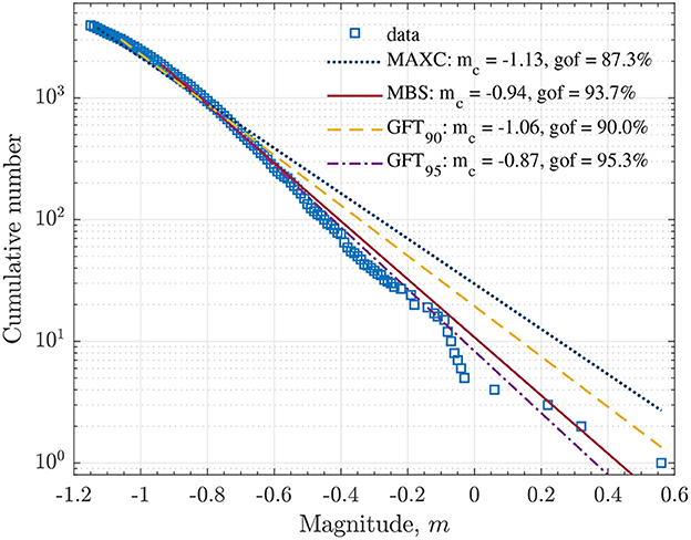
Figure 3. The frequency-magnitude statistics for the mining-induced seismicity. The light blue open squares represent the cumulative number of events. The distribution was fit by the G-R relation (3) with the cutoff magnitude mmin taken to be the completeness magnitude mc. Several fits correspond to different values of mc obtained from the application of: the MAXC (dotted blue line), MBS (solid red line), GFT (90% yellow dashed line), and GFT (95% purple doted-dashed line) methods. The estimated a and b-values with 95% confidence intervals are given in Table 1.
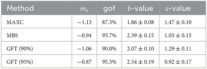
Table 1. The estimated magnitude of completeness mc, a and b-value with 95% confidence intervals using several methods.
To investigate any possible bi-modality in the frequency-magnitude statistics, the variability of event magnitudes were modeled by two other distributions. Specifically, we considered the tapered Pareto distribution (8) as well as the mixture of the tapered Pareto (8) and Pareto (6) distributions given in Equation (10). The obtained goodness-of-fit percentages vs. mc for each model are plotted in Supplementary Figure S4. Using the lower magnitude cutoff mmin = −0.94 the fits of the frequency-magnitude distribution are given in Figure 4. The estimated parameters with 95% confidence intervals are reported in Table 2 for each model. In addition, the fits of the three models are plotted in the seismic moment scale in Supplementary Figure S5. For comparison, we also plot in Supplementary Figures S6, S7 the results of the fit of the three models for the lower magnitude cutoff mmin = −1.5, and the values of the parameters are reported in Supplementary Table S1.
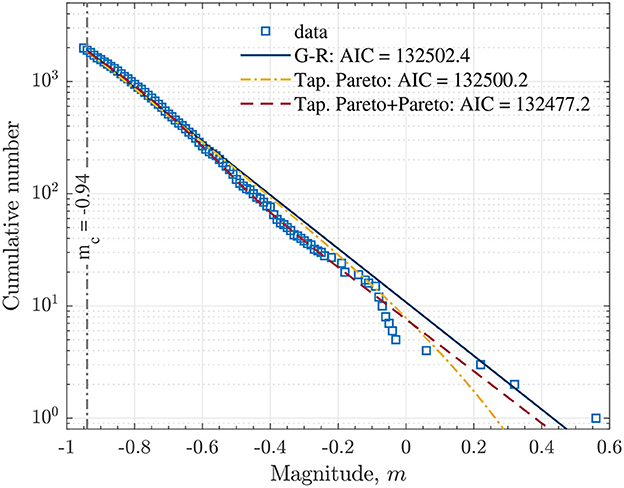
Figure 4. The frequency-magnitude statistics for the mining-induced seismicity. The blue open squares represent the cumulative number of events. The dark blue line is the fit of the G-R scaling (3). The dash-doted line is the fit of the tapered Pareto distribution (9). The dashed line is the fit of the mixture of the tapered Pareto and Pareto distributions (10).
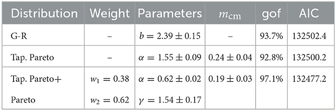
Table 2. The estimated model parameters with 95% confidence intervals for the three frequency-magnitude models applied to the mining microseismicity with the events above magnitude m ≥ −0.94.
The spatial dependence of the frequency-magnitude statistics was analyzed by subdividing the mine layout into several subregions (Supplementary Figure S8). The evolution of the cumulative numbers of events above magnitude m ≥ −0.94 is given in Supplementary Figure S9. For each subregion, the distribution of magnitudes was modeled using the exponential distribution (4). The results are illustrated in Supplementary Figure S10.
To investigate the Poisson nature of the occurrence of microseismicity, we analyzed the distribution of interevent times between successive events for the whole catalog. This distribution of interevent times for the events above magnitude mmin = −0.94 is plotted in Figure 5. The distribution was modeled separately by the exponential (1) and gamma (2) distributions. Based on the AIC or BIC the gamma distribution is a better fit to the distribution of interevent times. We also analyzed this distribution for different lower-magnitude cutoffs. Specifically, we considered mmin = −1.5, −1.3, −1.1, −0.9, and −0.7. The results are illustrated in Supplementary Figure S11.
Figure 5. The distribution of interevent times between successive events for all events above magnitude mmin = −0.94. The fits of the exponential distribution (blue dashed curve) and the gamma distribution (solid red curve) are given with corresponding model parameters and the values of AIC and BIC. The parameter uncertainties are reported with 95% confidence intervals.
To analyze the sequence further and establish whether it confirms Poisson or non-Poisson statistics, we computed the coefficient of variation , where σΔt is the standard deviation and 〈Δt〉 is the mean of the interevent times. The obtained value of COV = 1.54 indicates that the sequence deviates from Poisson statistics showing higher variability in the interevent times compared to the mean value. The values of the coefficient of variation above 1.0 typically indicate that time series tend to show a certain degree of clustering. In case of mining seismicity, this can be attributed to systematic changes in the underground stress field related to mining operations that induce microseismicity.
In addition, we also analyzed the distribution of magnitude differences between successive events: Δmi = mi − mi−1. In order to check any correlations between magnitudes, we considered the difference between the cumulative distributions: ΔP(dm) = P(Δm < dm) − P(Δm* < dm), where Δm* is the difference between magnitudes of the reshuffled catalogs [67]. The results are plotted in Figure 6. The dependence of the performed analysis on the lower magnitude cutoff is shown in Supplementary Figure S12. For the earthquake magnitudes that do not show significant correlations between the magnitudes, this difference ΔP(dm) should fluctuate around zero. However, the contrary is observed in case of the mining seismicity and indicates a positive correlation between magnitudes of subsequent events on short time scales. Similarly to the degree of clustering in the interevent data, this shows that subsequent events have comparable magnitudes on short time scales and indication of swarm-like behavior driven by mining.
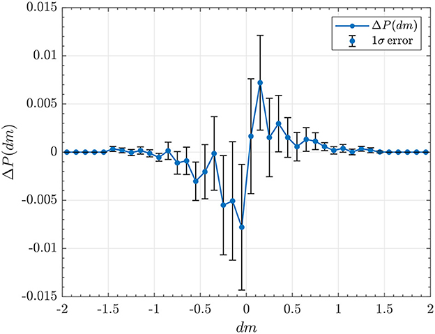
Figure 6. The dependence of the differences in cumulative magnitude distributions ΔP(dm) on the size difference dm between the magnitudes of subsequent events. The mean of the 1,000 reshuffled cataloge is considered for Δm*. The error bars correspond to one standard deviation.
To support the above results, we also performed a cross-correlation analysis of the seismicity rate and the corresponding mining activity in Subregion 2 of the mine shown in Supplementary Figure S8. The seismicity rate, R(t), was computed as the number of events above magnitude m = −0.94 occurring each day during the study period. The mining activity was computed as the number of hours per day the mine was performing the cutting operations. These two time-series are given in Figures 7A, B, respectively. For the cross-correlation analysis, the corresponding time series was computed by subtracting the mean from the seismicity rate and dividing by the standard deviation: . Similarly, the normalized time-series was computed for cutting operations: . By computing the cross-correlation function g(τ) = 〈r(t)c(t′)〉, where τ = t − t′ specifies a time lag, one can analyze any possible correlation between the two time-series. The results are given in Figure 7C as a plot of the cross-correlation coefficient vs. lag time in days. It clearly indicates that there are positive and negative correlations between the two time-series at certain time lags. To check this further, we randomly reshuffled the cutting operations time-series and repeated the same analysis. This is given in Supplementary Figure S13, which shows the disappearance of any correlations present in the original time-series.
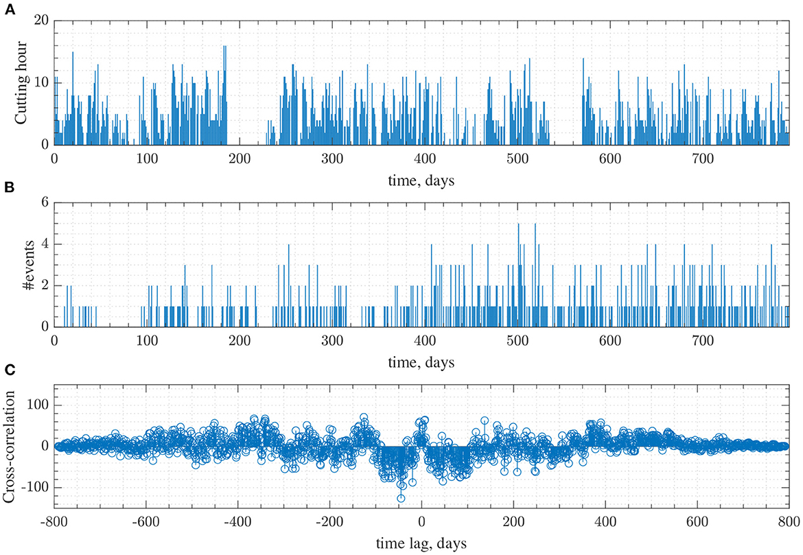
Figure 7. Cross-correlation analysis between microseismicity rate and the mine cutting operation rate in Subregion 2 of the mine. (A) The mine-cutting operations are given as the number of cutting hours per day. (B) The seismicity rate is computed as the number of events above magnitude m = −0.94 per day. (C) The cross-correlation coefficient vs. time lag is given.
In addition to the interevent time analysis, the clustering of induced mining seismicity was analyzed using the NND method, which also takes into account the spatial distribution of events. In this analysis, we used b = 2.39, df = 1.6, and considered the epicentral distances between events with the magnitudes above mmin = −0.94 when computing the rescaled times (14) and distances (15). The obtained distributions of the rescaled distances R and times T as well as the nearest-neighbor proximity η are given in Figure 8.
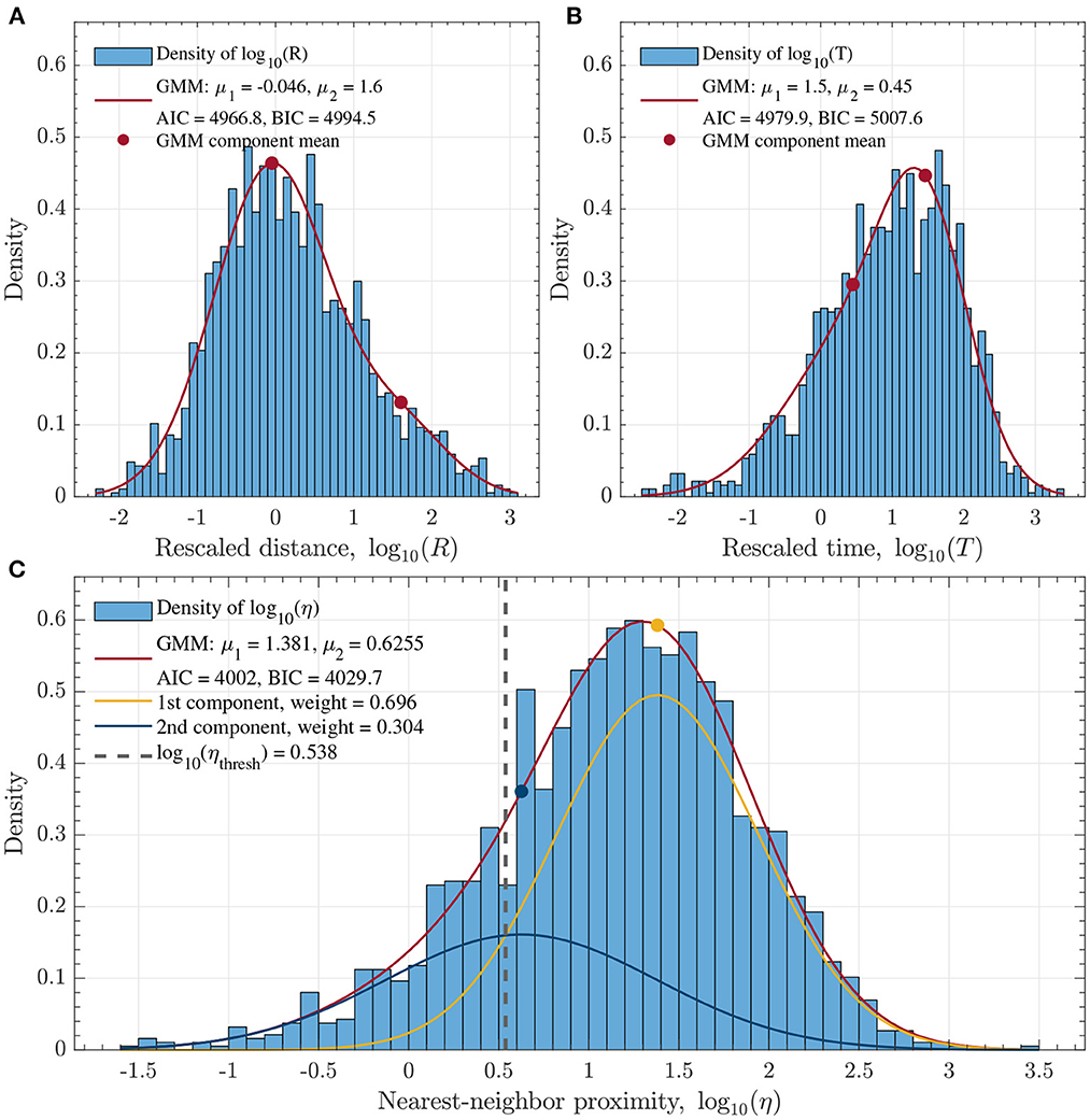
Figure 8. The distributions of the (A) rescaled distances R, (B) rescaled times T, and (C) nearest-neighbor proximity ηj for all events above magnitude m ≥ −0.94. The dark red curves are the fits of the two-component Gaussian mixture model to each distribution. The individual components are shown in (C) as yellow and blue solid curves with the corresponding means and weights given in the legend. The threshold log10 (ηthresh) = 0.538 was estimated from the intersection of the two components and is shown as a vertical dashed line.
The multi-modality of the distribution of η was studied by fitting the Gaussian mixture model (GMM). The fit of the two-component GMM is given in Figure 8. The comparison of the GMM fits with the number of components ranging between 1 and 4 is given in Supplementary Figure S14. The Bayesian information criterion (BIC) was used for model selection. As a result, the GMM with the two components had the lowest BIC = 4029.7. This result illustrates that the microseismic events can be declustered into two classes, i.e. the background events and clustered events. The intersect of the two components of the selected GMM was considered as a threshold for the log10 ηthresh = 0.538 value in the declustering process (Figure 8).
In order to investigate the characteristics of possible clustering modes, the joint normalized distribution of the rescaled spatial R and temporal T components is plotted in Figure 9. The dashed white line corresponds to the threshold log10 ηthresh = 0.538 chosen as the intersection of the two components of the GMM fit.
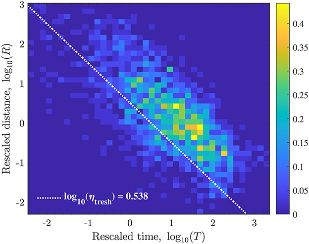
Figure 9. The normalized density plot of the joint distribution of the rescaled time T and space R. The white dashed line corresponds to the threshold log10(ηthresh) = 0.538.
In the analysis of the rescaled nearest-neighbor distances η, we showed that the distribution of η can be fitted by the two-component GMM and the intersect of the two components was used to obtain a threshold value of log10 ηthresh = 0.538 (Figure 8). This threshold value ηthresh was used to separate the clustered seismicity from the background seismicity. The clustered events are considered those for which R + T < ηthresh (Figure 9 and Supplementary Figure S15). In addition, we also introduced two more constraints on the maximum distance and maximum time interval between nearest-neighbor events. Specifically, we assumed that events cannot be linked if they were more than 100 days apart and separated by more than 5 km. This allowed us to separate events into two main categories, i.e. the background events that lie to the right from the white dashed line given in Figure 9 and Supplementary Figure S15 and the clustered events that have parent events.
As a result of this declustering, 1,407 events that were separated from their parent events formed the background (singleton) events and the rest 488 events formed the clustered events (Supplementary Figure S16). This also resulted in the formation of a total of 157 family trees with clusters containing more than one event. The NND method subdivided the analyzed sequence into 14 classes (Figure 10B). The largest cluster was formed by the largest event in the catalog with the local magnitude of m = 0.56 (Supplementary Figure S16d).
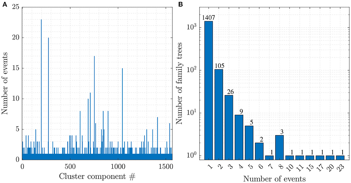
Figure 10. Cluster statistics is shown for (A) the number of events in each cluster and (B) the distribution of clusters according to the number of nodes.
Out of 157 tree families, nine families had more than seven events (Supplementary Figure S16c). The first nine largest clusters are shown in Supplementary Figure S17. Each node is labeled by the corresponding event magnitude. Several cluster characteristics are also provided. These include: the number of events in each cluster N, the cluster duration in days Td, the difference between the largest (root) and the second largest event Δm, the average leaf depth 〈d〉, the normalized leaf depth , and the inverted branching number BI [49, 53].
The spatial distribution of each cluster tree is plotted in Figure 11. Since clustered events are separated by the rescaled distance less than log10 η < 0.538, most of the family members are very close to each other in the spatio-temporal space. In Supplementary Figure S18, the plot of the magnitudes vs. time for each tree is plotted. Finally, the spatial distribution of all the clusters and background events are plotted on top of the mine layout (Figure 12) and the corresponding magnitude vs. time structure (Supplementary Figure S22).
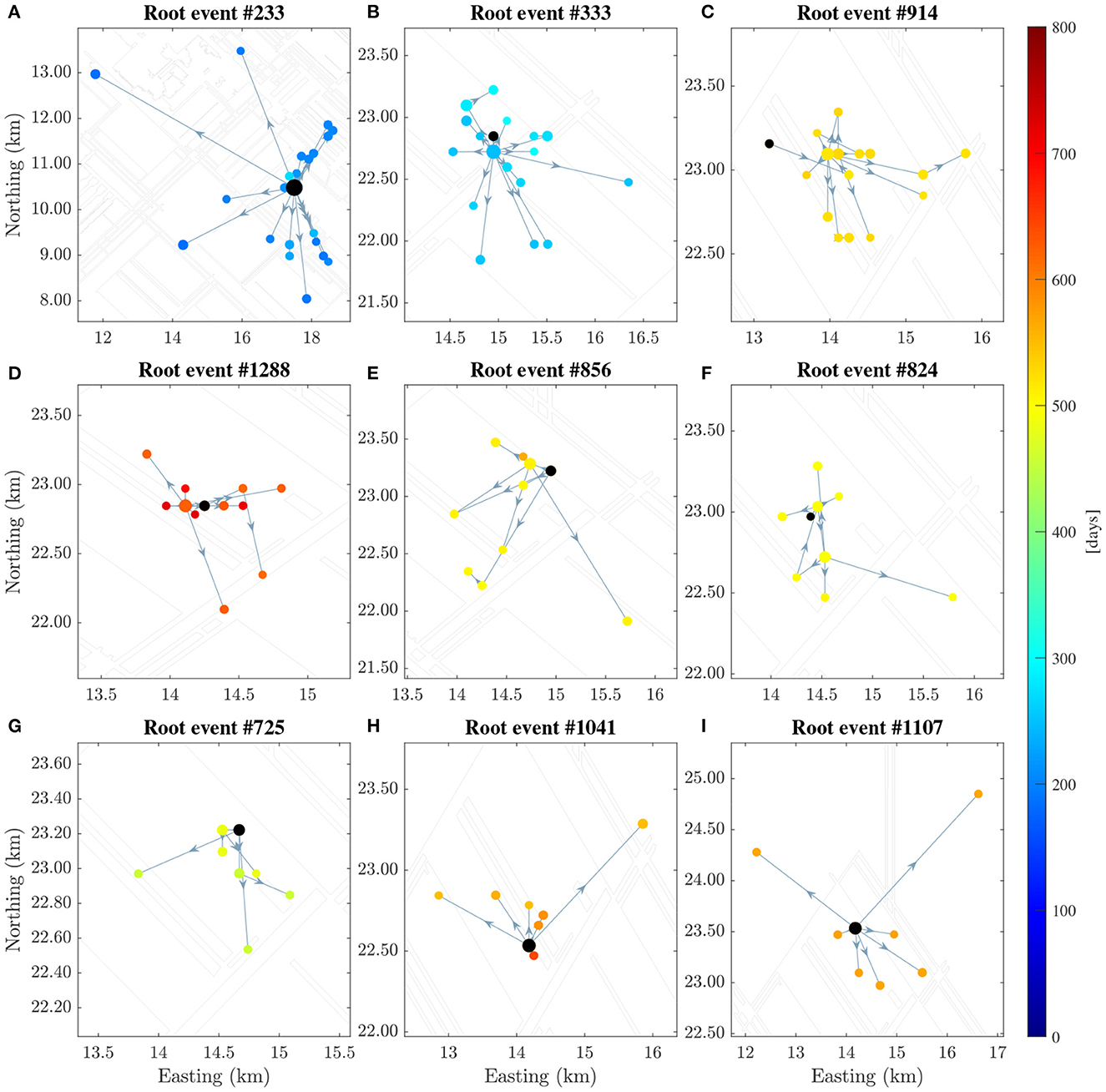
Figure 11. The spatial distribution of the nine largest clusters with respect to the mine layout. The panels from (A)-(I) correspond to the clusters initiated by the root events (the black solid circles) indicated by their numbers in the catalog.
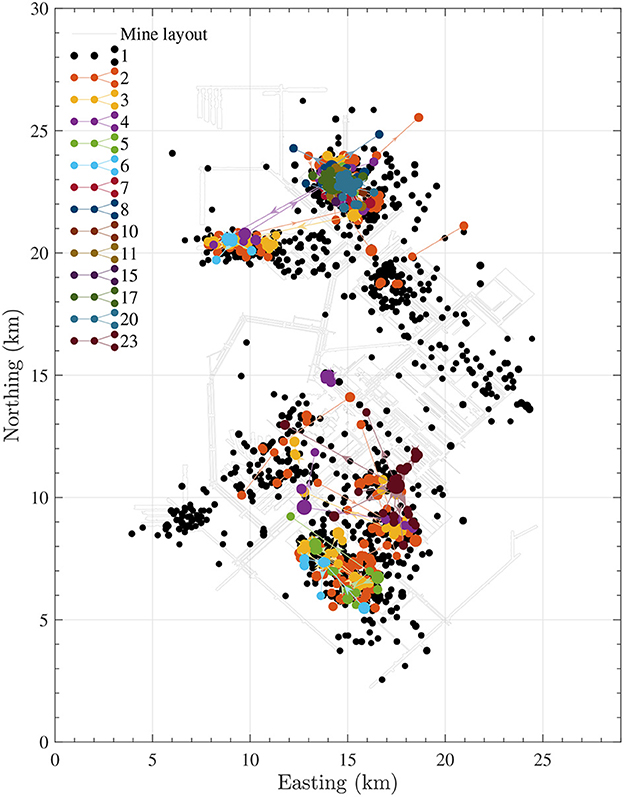
Figure 12. The spatial distribution of all the clusters identified using the NND method by using the threshold log10(ηthresh) = 0.538. This is plotted with respect to the mine layout. Black solid circles indicate the singleton events. The colored solid circles are all clusters with more than one event.
The statistical analysis is crucial to quantify patterns of seismic activity and provides insight into possible physical mechanisms that are responsible for triggering of mining microseismicity. It is standard practice to assume that the occurrence of seismic events can be approximated by a stochastic marked point process in time and space. This approximation assumes that seismic events are governed by certain statistical models in temporal, spatial, and magnitude domains. The approach undertaken in this work was to establish and apply these statistical models to mining microseismicity in order to make specific inferences about the physical and statistical properties of the mine host-rock environment.
When working with a microseismic catalog, one encounters a standard problem of the incompleteness of the catalog below a certain magnitude mc. The underestimation of this threshold magnitude can introduce a significant bias in the statistical results. Therefore, we performed a comprehensive analysis to establish the magnitude of the completeness for the mining catalog we used in this study. Specifically, we employed the method of maximum curvature (MAXC), the method of b-value stability analysis (MBS), and the method based on the goodness-of-fit test (GFT). The details of the methods used are summarized in Section 3.3. We applied these methods by first assuming that the event magnitude distribution can be described by the left-truncated exponential distribution (4) or a more commonly accepted form of G-R scaling (3). The MBS and GFT methods produced a consistent estimate for the magnitude of the completeness mc. The MAXC method is known to underestimate mc, typically, by 0.2 magnitude units. Therefore, we decided to use the value of mc = −0.94 from the MBS method as it is somewhere in between of the two values returned by the GFT method. This gives that 93.7% of the distribution of magnitudes above mc = −0.94 can be explained by the G-R fit (Figure 3) and this value of mc was adopted for the subsequent analysis.
When fitting the distribution of event magnitudes above m ≥ −0.94 with the exponential model (4), we obtained a rather large value for β = 5.5 ± 0.35 or corresponding b = 2.39 ± 0.15. This indicates that the mining microseismicity is distributed over a narrow range of magnitudes above the completeness level and displays swarm-like characteristics. An earthquake swarm is typically characterized by the occurrence of events of similar magnitude sizes. This can be related to the fact that the microseismicity is driven primarily by mining operations and is occurring on newly created fractures with a limited size distribution [68]. This also indicates that the frequency-magnitude statistics in soft rock environment differs from what is typically observed in hard rock settings [28, 69]. The observed higher than typical tectonic b-values were also observed in other instances of induced seimsmicity [70, 71]. b-value can also be indicative of the state of stress in the crust [72–75]. In tectonic settings, high b-values are typically associated with an extensional stress regime resulting in predominantly normal faulting for seismic events [76]. One possible explanation for the obtained high b-value result is the occurrence of events in ductile rock environment as was suggested by [72] for rock fracture experiments.
To investigate this further, we performed a cross-correlation analysis between the microseismicity rate and the corresponding mine-cutting operations in one particular subregion of the mine. The computed cross-correlation coefficient clearly shows a pattern of negative and positive correlations between the two time-series (Figure 7). The pattern disappears when the cutting time-series was randomly reshuffled (Supplementary Figure S13). In addition, most of the events occurred at rather shallow depths in soft rock environments without the presence of any major fault structures. The performed cross-correlation analysis does not fully explain what kind of mechanisms are responsible for triggering of the microseismicity. The main limitation is that the cutting rate is only a proxy for the actual mining operations. In addition, it may provide an indirect indication that some delayed triggering mechanism is also present influenced by the ductile deformation of soft rock material.
The left-truncated exponential distribution (4) or its equivalent, G-R scaling (3), is the most commonly used model to describe the frequency-magnitude statistics of earthquakes. However, the actual magnitude distribution of mining seismicity can deviate from G-R scaling and can exhibit a bimodality or other features. Therefore, we explored several other possible statistical models to fit the observed distribution of event magnitudes. Specifically, we considered the tapered Pareto distribution (8) when the magnitude m is replaced by the corresponding scalar seismic moment M = 101.5(m+10.73). We also considered the mixture of the tapered Pareto and Pareto distributions (10).
The application of the goodness-of-fit test indicates that the mixture of the tapered Pareto and Pareto distributions, Equation (10), can fit better the frequency-magnitude statics over a wider range of magnitudes lowering the completeness level to mc = −1.5 (Supplementary Figures S4, S6, S7). However, this still does not fully resolve the problem that the microseismic events are fully recorded in the catalog up to this level. The histogram of the distribution of microseismic event magnitudes, given in Supplementary Figure S1, shows that there is a decrease in the number of events in each magnitude bin below the value m = −1.1. This indicates the deficiency in the numbers below this level and is typically attributed to the incompleteness of a catalog. When fitting all the three models and considering only events above magnitude mmin = −0.94, the exponential distribution (4) and the mixture of the tapered Pareto and Pareto distributions, Equation (10), fit the data best (Figure 4 and Supplementary Figure S5).
The event occurrence rate is a direct manifestation of the underlying physical processes responsible for the induction or triggering of microseismic events. The analysis of the mining seismicity shows that it is primarily controlled by the mining operations and lack any significant aftershock sequences. The cumulative number of events given in Figure 2 shows the almost steady linear increase with time for events above m ≥ −0.94 indicating a relatively constant rate of occurrence. However, the interevent time distribution between consecutive events (Figure 5) shows a deviation from the exponential distribution for short time intervals and is better described by the gamma distribution. This signifies that events that are separated by time intervals shorter than 10 min are driven by the time-dependent rate related to the mining operations. This is also observed by studying the distribution of the magnitude difference between consecutive events (Figure 6). This distribution shows a clear correlation between consecutive magnitudes and an indication of deviation from Poisson statistics on shorter time scales. However, it is also affected by the magnitude completeness of the catalog and the effect is more pronounced for lower magnitude cutoffs (Supplementary Figure S12). This effect was also observed in case of rock fracture experiments [20]. A related approach was recently suggested to use the difference between consecutive magnitudes to estimate the b-value that can handle the catalog incompleteness more efficiently [77]. However, that method relies on the assumption that the earthquake magnitudes are independent. In the case of mining seismicity, our analysis indicates a short-time correlation between magnitudes.
Clustering of seismicity is an invaluable feature that is directly related to the mechanisms of triggering and interaction between seismic events. In our work, we used the NND method (Section 3.4) to identify characteristics of the triggering process and the structure of event family trees. The GMM was utilized to investigate any possible multimodality in the distribution of the rescaled nearest-neighbor proximity between events, η (Figure 8). The GMM with two components achieved the lowest BIC = 4029.7 (Supplementary Figure S14). The corresponding intersection of the two components of the GMM was used to identify the threshold, η = 0.538, in the declustering process (Figure 8). Therefore, the microseismic events can be classified as being background events (isolated singleton events) or as clustered events. The obtained results show that the analyzed microseismic catalog has characteristics that are dominated by the occurrence of isolated singleton events.
Within the NND analysis, seismic family trees that form the clustered events can be subdivided into three main types: swarm-like, burst-type, or aftershocks [48, 49]. The swarm-like families are those chains of seismic events without branches. The burst-type families are those that have only one parent event and many children. The aftershock-type families are the combination of both mentioned types and contain first or higher-order triggered events. By applying this classification to the mining microseismicity we were able to identify 52 families (groups of microseismic events) that had more than two nodes. Using the criterion based on the value of BI (BI = 1 – swarm-type, BI > 0.5 – aftershock-type, and BI ≤ 0.5 – burst-type), from these 52 seismic family trees, 18 families had swarm-type, eight family trees had aftershock-type, and the rest had burst-type characteristics (Supplementary Figures S19–S21). This indicates that among clustered events the “burst-type” of activity dominates the clustering. It should be mentioned from these 52 family trees, 17 families had a foreshock sequence, and in the other 35 families, the root event was the largest event in the family tree. As the cluster size distribution is dominated by small clusters with a predominantly “burst-type” structure (Figure 10), the cluster leaf depth is typically short.
In this work, several statistical methods were applied to investigate the nature of microseismicity in a potash mine in Saskatchewan, Canada. Specifically, the modeling of the frequency-magnitude statistics was performed by fitting several models: the left-truncated exponential distribution (or equivalently G-R scaling), the tapered Pareto distribution, and their mixtures. By analyzing the rate of seismicity we concluded that the occurrence of events deviates from Poisson statistics on short time scales and for the lower magnitude cutoffs. The magnitude of completeness was estimated using several methods and we used mc = −0.94 for the analysis. The results of the clustering analysis of microseismicity indicate that the majority of events can be treated as independent background events mostly driven by underground mining operations. However, there is some clustering of seismicity and the formation of limited aftershock sequences. This clustering is predominantly of “burst-type” in the terminology adopted in the NND analysis.
From the analysis performed in this work, we can draw several specific conclusions concerning the observed mining microseismicity. The frequency-magnitude distribution of seismicity exhibits a relatively high b-value (b = 2.39 ± 0.15) indicating that the seismic events are distributed in a rather narrow magnitude range above the completeness threshold m ≥ −0.94. The largest observed event during the study period had a magnitude of 0.56. The interevent triggering is also suppressed and does not show any significant cascade-like propagation of seismicity. This suggests that the probability of having even larger events is very low and does not constitute a significant hazard for the safe operation of the mine.
The data analyzed in this study is subject to the following licenses/restrictions. The earthquake catalog supporting this research is not publicly available due to confidentiality restrictions imposed by Nutrien Ltd. A research request to access the catalog data can be made to Nutrien Ltd. by following an appropriate protocol. Requests to access these datasets should be directed at: Nutrien Ltd., https://www.nutrien.com/.
MS performed research, analyzed data, wrote the computer code, wrote the manuscript, and handled the submission. MB provided the data characteristics, participated in discussions, and provided comments and contributed to the writing of the manuscript. RS formulated the problem, supervised the research, wrote the manuscript and computer code, analyzed data, and acquired funding. All authors contributed to the article and approved the submitted version.
The work has been supported by the Accelerate grant from Mitacs and International Minerals Innovation Institute to study mining microseismicity. RS also acknowledges support from NSERC through the Discovery grant.
We acknowledge Nutrien Ltd.'s permission to use the mining microseismicity catalog. We would like to thank Haroldo Ribeiro and Leila Mizrahi for their constructive and helpful critique of the manuscript that helped to improve the presentation and clarify results.
MB was employed by Nutrien Ltd.
The remaining authors declare that the research was conducted in the absence of any commercial or financial relationships that could be construed as a potential conflict of interest.
All claims expressed in this article are solely those of the authors and do not necessarily represent those of their affiliated organizations, or those of the publisher, the editors and the reviewers. Any product that may be evaluated in this article, or claim that may be made by its manufacturer, is not guaranteed or endorsed by the publisher.
The Supplementary Material for this article can be found online at: https://www.frontiersin.org/articles/10.3389/fams.2023.1126952/full#supplementary-material
2. Lasocki S, Orlecka-Sikora B. Seismic hazard assessment under complex source size distribution of mining-induced seismicity. Tectonophysics. (2008) 456:28–37. doi: 10.1016/j.tecto.2006.08.013
3. Gibowicz SJ, Lasocki S. Seismicity induced by mining: ten years later. Adv Geophys. (2000) 44:39–181. doi: 10.1016/S0065-2687(00)80007-2
4. Gibowicz SJ. Seismicity induced by mining: recent research. Adv Geophys. (2009) 51:1–53. doi: 10.1016/S0065-2687(09)05106-1
5. Gendzwill DJ, Horner RB, Hasegawa HS. Induced earthquakes at a potash mine near Saskatoon, Canada. Can J Earth Sci. (1982) 19:466–75. doi: 10.1139/e82-038
6. Riemer KL, Durrheim RJ. Mining seismicity in the Witwatersrand Basin: monitoring, mechanisms and mitigation strategies in perspective. J Rock Mech Geotech Eng. (2012) 4:228–49. doi: 10.3724/SP.J.1235.2012.00228
7. Li Y, Yang TH, Liu HL, Wang H, Hou XG, Zhang PH, et al. Real-time microseismic monitoring and its characteristic analysis in working face with high-intensity mining. J Appl Geophys. (2016) 132:152–63. doi: 10.1016/j.jappgeo.2016.07.010
8. Ghosh GK, Sivakumar C. Application of underground microseismic monitoring for ground failure and secure longwall coal mining operation: a case study in an Indian mine. J Appl Geophys. (2018) 150:21–39. doi: 10.1016/j.jappgeo.2018.01.004
9. Ellsworth WL. Injection-induced earthquakes. Science. (2013) 341:1225942. doi: 10.1126/science.1225942
10. Atkinson GM, Eaton DW, Ghofrani H, Walker D, Cheadle B, Schultz R, et al. Hydraulic fracturing and seismicity in the western Canada sedimentary basin. Seismol Res Lett. (2016) 87:631–47. doi: 10.1785/0220150263
11. Schultz R, Skoumal RJ, Brudzinski MR, Eaton D, Baptie B, Ellsworth W. Hydraulic fracturing-induced seismicity. Rev Geophys. (2020) 58:e2019RG000695. doi: 10.1029/2019RG000695
12. Hasegawa HS, Wetmiller RJ, Gendzwill DJ. Induced seismicity in mines in Canada-An overview. Pure Appl Geophys. (1989) 129:423–53. doi: 10.1007/978-3-0348-9270-4_10
13. Gendzwill DJ, Stead D. Rock mass characterization around Saskatchewan potash mine openings using geophysical techniques-a review. Can Geotech J. (1992) 29:666–74. doi: 10.1139/t92-073
14. Funk C, Lsbister J, LeBlanc T, Brehm R. Mapping how geophysics is used to understand geohazards in potash mines. CSEG Record. (2019) 44:1–6.
15. Roche V, van der Baan M. The role of lithological layering and pore pressure on fluid-induced microseismicity. J Geophys Res. (2015) 120:923–43. doi: 10.1002/2014JB011606
16. Gibowicz SJ, Young RP, Talebi S, Rawlence DJ. Source parameters of seismic events at the underground research laboratory in Manitoba, Canada: scaling relations for events with moment magnitude smaller than -2. Bull Seismol Soc Am. (1991) 81:1157–82.
17. Gendzwill DJ. Induced seismicity in Saskatchewan potash mines. In:Gay NC, Wainwright EH, , editors. The 1st International Congress on Rockbursts and Seismicity in Mines. Johannesburg: SAIMM (1984), p. 131–46.
18. Baro J, Corral A, Illa X, Planes A, Salje EKH, Schranz W, et al. Statistical similarity between the compression of a porous material and earthquakes. Phys Rev Lett. (2013) 110:088702. doi: 10.1103/PhysRevLett.110.088702
19. Ribeiro HV, Costa LS, Alves LGA, Santoro PA, Picoli S, Lenzi EK, et al. Analogies between the cracking noise of ethanol-dampened charcoal and earthquakes. Phys Rev Lett. (2015) 115:025503. doi: 10.1103/PhysRevLett.115.025503
20. Davidsen J, Kwiatek G, Charalampidou EM, Goebel T, Stanchits S, Ruck M, et al. Triggering processes in rock fracture. Phys Rev Lett. (2017) 119:068501. doi: 10.1103/PhysRevLett.119.068501
21. Dunn CE,. Geology of the middle devonian dawson bay formation in the saskatoon potash mining district, Saskatchewan (MSc thesis). Saskatchewan Geological Survey, Regina, SK, Canada. (1982). Available online at: https://searchworks.stanford.edu/view/1662929
23. Funk C, Derkach J, MacKenzie L. Lanigan potash deposit. Tech. Rep. KLSA 001 C, Nutrien Ltd. (2019). Natinal Instrument 43-101 Technical Report. Available online at: https://minedocs.com/22/Lanigan-TR-12312021.pdf
24. Sepehr K, Stimpson B. Potash mining and seismicity-A time-dependent finite-element model. Int J Rock Mech Min Sci. (1988) 25:383–92. doi: 10.1016/0148-9062(88)90978-3
25. Gibowicz SJ, Kijko A. An Introduction to Mining Seismology. San Diego, CA: Academic Press (1994).
26. Boltz MS, Pankow KL, McCarter MK. Fine details of mining-induced seismicity at the Trail Mountain Coal Mine using modified hypocentral relocation techniques. Bull Seismol Soc Am. (2014) 104:193–203. doi: 10.1785/0120130011
27. Richardson E, Jordan TH. Seismicity in deep gold mines of South Africa: implications for tectonic earthquakes. Bull Seismol Soc Am. (2002) 92:1766–82. doi: 10.1785/0120000226
28. Kgarume TE, Spottiswoode SM, Durrheim RJ. Statistical properties of mine tremor aftershocks. Pure Appl Geophys. (2010) 167:107–17. doi: 10.1007/s00024-009-0004-5
29. Lasocki S. Statistical estimation of the efficiency of earthquake prediction under uncertain identification of target events. Bull Seismol Soc Am. (2000) 90:324–33. doi: 10.1785/0119980098
30. Martinsson J, Törnman W. Modelling the dynamic relationship between mining induced seismic activity and production rates, depth and size: a mine-wide hierarchical model. Pure Appl Geophys. (2020) 177:2619–39. doi: 10.1007/s00024-019-02378-y
31. Lasocki S, Orlecka-Sikora B. Anthropogenic seismicity related to exploitation of georesources. In:Gupta HK, , editor. Encyclopedia of Solid Earth Geophysics. Cham: Springer (2020), p. 1–8. doi: 10.1007/978-3-030-10475-7_277-1
32. Vallejos JA, McKinnon SD. Correlations between mining and seismicity for re-entry protocol development. Int J Rock Mech Min Sci. (2011) 48:616–25. doi: 10.1016/j.ijrmms.2011.02.014
33. Vallejos JA, Estay RA. Seismic parameters of mining-induced aftershock sequences for re-entry protocol development. Pure Appl Geophys. (2018) 175:793–811. doi: 10.1007/s00024-017-1709-5
34. Vallejos JA, McKinnon SD. Omori's law applied to mining-induced seismicity and re-entry protocol development. Pure Appl Geophys. (2010) 167:91–106. doi: 10.1007/s00024-009-0010-7
35. Aggarwal CC, Reddy CK. Data Clustering: Algorithms and Applications. Boca Raton, FL: Chapman and Hall/CRC (2014).
36. Bouveyron C, Celeux G, Murphy TB, Raftery AE. Model-based Clustering and Classification for Data Science: With Applications in R. New York, NY: Cambridge University Press (2019). doi: 10.1017/9781108644181
37. Frohlich C, Davis SD. Single-link cluster-analysis as a method to evaluate spatial and temporal properties of earthquake catalogs. Geophys J Int. (1990) 100:19–32. doi: 10.1111/j.1365-246X.1990.tb04564.x
38. Kijko A, Lasocki S, Retief SJP. Identification of Rock Mass Discontinuities in a Cluster of Seismic Event Hypocenters. Safety Mines Research Advisory Committee (1999). p. 1–20.
39. Hudyma MR. Analysis and Interpretation of Clusters of Seismic Events in Mines. PhD thesis. University of Western Australia Perth (2008).
40. Leśniak A, Isakow Z. Space-time clustering of seismic events and hazard assessment in the Zabrze-Bielszowice coal mine, Poland. Int J Rock Mech Min Sci. (2009) 46:918–28. doi: 10.1016/j.ijrmms.2008.12.003
41. Woodward K, Wesseloo J, Potvin Y. A spatially focused clustering methodology for mining seismicity. Eng Geol. (2018) 232:104–13. doi: 10.1016/j.enggeo.2017.11.015
42. Ester M, Kriegel HP, Sander J, Xu X. A density-based algorithm for discovering clusters in large spatial databases with noise. KDD-96. (1996) 96:226–31.
43. Meyer SG, Bassom AP, Reading AM. Delineation of fault segments in mines using seismic source mechanisms and location uncertainty. J Appl Geophys. (2019) 170:103828. doi: 10.1016/j.jappgeo.2019.103828
44. Lurka A. Spatio-temporal hierarchical cluster analysis of mining-induced seismicity in coal mines using Ward's minimum variance method. J Appl Geophys. (2021) 184:104249. doi: 10.1016/j.jappgeo.2020.104249
45. Mizrahi L, Nandan S, Wiemer S. The effect of declustering on the size distribution of mainshocks. Seismol Res Lett. (2021) 92:2333–42. doi: 10.1785/0220200231
46. Baiesi M, Paczuski M. Scale-free networks of earthquakes and aftershocks. Phys Rev E. (2004) 69:066106. doi: 10.1103/PhysRevE.69.066106
47. Zaliapin I, Gabrielov A, Keilis-Borok V, Wong H. Clustering analysis of seismicity and aftershock identification. Phys Rev Lett. (2008) 101:018501. doi: 10.1103/PhysRevLett.101.018501
48. Zaliapin I, Ben-Zion Y. Earthquake clusters in southern California I: identification and stability. J Geophys Res. (2013) 118:2847–64. doi: 10.1002/jgrb.50179
49. Zaliapin I, Ben-Zion Y. A global classification and characterization of earthquake clusters. Geophys J Int. (2016) 207:608–34. doi: 10.1093/gji/ggw300
50. Zaliapin I, Ben-Zion Y. Earthquake declustering using the nearest-neighbor approach in space-time-magnitude domain. J Geophys Res. (2020) 125:e2018JB017120. doi: 10.1029/2018JB017120
51. Maghsoudi S, Eaton DW, Davidsen J. Nontrivial clustering of microseismicity induced by hydraulic fracturing. Geophys Res Lett. (2016) 43:10672–9. doi: 10.1002/2016GL070983
52. Maghsoudi S, Baro J, Kent A, Eaton D, Davidsen J. Interevent triggering in microseismicity induced by hydraulic fracturing. Bull Seismol Soc Am. (2018) 108:1133–46. doi: 10.1785/0120170368
53. Kothari S, Shcherbakov R, Atkinson G. Statistical modeling and characterization of induced seismicity within the Western Canada Sedimentary Basin. J Geophys Res. (2020) 125:e2020JB020606. doi: 10.1029/2020JB020606
54. Shcherbakov R, Yakovlev G, Turcotte DL, Rundle JB. Model for the distribution of aftershock interoccurrence times. Phys Rev Lett. (2005) 95:218501. doi: 10.1103/PhysRevLett.95.218501
55. Corral Á. Long-term clustering, scaling, and universality in the temporal occurrence of earthquakes. Phys Rev Lett. (2004) 92:108501. doi: 10.1103/PhysRevLett.92.108501
56. Utsu T, Ogata Y, Matsu'ura RS. The centenary of the Omori formula for a decay law of aftershock activity. J Phys Earth. (1995) 43:1–33. doi: 10.4294/jpe1952.43.1
57. Gutenberg B, Richter CF. Frequency of earthquakes in California. Bull Seismol Soc Am. (1944) 4:185–8. doi: 10.1785/BSSA0340040185
58. Vere-Jones D. Foundations of statistical seismology. Pure Appl Geophys. (2010) 167:645–53. doi: 10.1007/s00024-010-0079-z
59. Bender B. Maximum likelihood estimation of b values for magnitude grouped data. Bull Seismol Soc Am. (1983) 73:831–51. doi: 10.1785/BSSA0730030831
60. Tinti S, Mulargia F. Confidence intervals of b-values for grouped magnitudes. Bull Seismol Soc Am. (1987) 77:2125–34.
61. Kagan YY. Seismic moment distribution revisited: I. Statistical results. Geophys J Int. (2002) 148:520–41. doi: 10.1046/j.1365-246x.2002.01594.x
62. Wiemer S, Wyss M. Minimum magnitude of completeness in earthquake catalogs: examples from Alaska, the western United States, and Japan. Bull Seismol Soc Am. (2000) 90:859–69. doi: 10.1785/0119990114
63. Cao AM, Gao SS. Temporal variation of seismic b-values beneath northeastern Japan island arc. Geophys Res Lett. (2002) 29:1334. doi: 10.1029/2001GL013775
64. Woessner J, Wiemer S. Assessing the quality of earthquake catalogues: estimating the magnitude of completeness and its uncertainty. Bull Seismol Soc Am. (2005) 95:684–98. doi: 10.1785/0120040007
65. Feng Y, Mignan A, Sornette D, Li J. Hierarchical Bayesian modeling for improved high-resolution mapping of the completeness magnitude of earthquake catalogs. Seismol Res Lett. (2022) 93:2126–37. doi: 10.1785/0220210368
66. Kosobokov VG, Mazhkenov SA. On similarity in the spatial distribution of seismicity. Comp Seism Geodyn. (1994) 1:6–15. doi: 10.1029/CS001p0006
67. Shcherbakov R, Davidsen J, Tiampo KF. Record-breaking avalanches in driven threshold systems. Phys Rev E. (2013) 87:052811. doi: 10.1103/PhysRevE.87.052811
68. Prugger A. The Fracture Mechanism of Weak Seismic Events near Potash Mines. PhD thesis. The University of Saskatchewan, Canada (1994).
69. Bhattacharya P, Phan M, Shcherbakov R. Statistical analysis of the 2002 Mw 7.9 Denali earthquake. Bull Seismol Soc Am. (2011) 101:2662–74. doi: 10.1785/0120100336
70. Dohmen T, Zhang J, Barker L, Blangy JP. Microseismic magnitudes and b-values for delineating hydraulic fracturing and depletion. SPE J. (2017) 22:1624–34. doi: 10.2118/186096-PA
71. Igonin N, Zecevic M, Eaton DW. Bilinear magnitude-frequency distributions and characteristic earthquakes during hydraulic fracturing. Geophys Res Lett. (2018) 45:12866–74. doi: 10.1029/2018GL079746
72. Scholz CH. The frequency-magnetude relation of microfracturing in rock and its relation to earthquakes. Bull Seismol Soc Am. (1968) 58:399–415. doi: 10.1785/BSSA0580010399
73. Bhattacharya P, Shcherbakov R, Tiampo KF, Mansinha L. Anomalous statistics of aftershock sequences generated by supershear ruptures. Res Geophys. (2012) 2:e6. doi: 10.4081/rg.2012.e6
74. Spada M, Tormann T, Wiemer S, Enescu B. Generic dependence of the frequency-size distribution of earthquakes on depth and its relation to the strength profile of the crust. Geophys Res Lett. (2013) 40:709–14. doi: 10.1029/2012GL054198
75. Tormann T, Wiemer S, Mignan A. Systematic survey of high-resolution b value imaging along Californian faults: inference on asperities. J Geophys Res. (2014) 119:2029–54. doi: 10.1002/2013JB010867
76. Schorlemmer D, Wiemer S, Wyss M. Variations in earthquake-size distribution across different stress regimes. Nature. (2005) 437:539–42. doi: 10.1038/nature04094
Keywords: mining seismicity, statistical seismology, nearest-neighbor distance, earthquake clustering, frequency-magnitude statistics
Citation: Sedghizadeh M, van den Berghe M and Shcherbakov R (2023) Statistical and clustering analysis of microseismicity from a Saskatchewan potash mine. Front. Appl. Math. Stat. 9:1126952. doi: 10.3389/fams.2023.1126952
Received: 18 December 2022; Accepted: 13 March 2023;
Published: 30 March 2023.
Edited by:
Jiancang Zhuang, Institute of Statistical Mathematics, JapanReviewed by:
Leila Mizrahi, ETH Zürich, SwitzerlandCopyright © 2023 Sedghizadeh, van den Berghe and Shcherbakov. This is an open-access article distributed under the terms of the Creative Commons Attribution License (CC BY). The use, distribution or reproduction in other forums is permitted, provided the original author(s) and the copyright owner(s) are credited and that the original publication in this journal is cited, in accordance with accepted academic practice. No use, distribution or reproduction is permitted which does not comply with these terms.
*Correspondence: Mohammadamin Sedghizadeh, bXNlZGdoaXpAdXdvLmNh
Disclaimer: All claims expressed in this article are solely those of the authors and do not necessarily represent those of their affiliated organizations, or those of the publisher, the editors and the reviewers. Any product that may be evaluated in this article or claim that may be made by its manufacturer is not guaranteed or endorsed by the publisher.
Research integrity at Frontiers
Learn more about the work of our research integrity team to safeguard the quality of each article we publish.