Stochastic time-optimal control and sensitivity studies for additional food provided prey-predator systems involving Holling type-IV functional response

In this study we consider an additional food provided prey-predator model exhibiting Holling type-IV functional response incorporating the combined effects of both the continuous white noise and discontinuous Lévy noise. We prove the existence and uniqueness of global positive solutions for the proposed model. We perform the stochastic sensitivity analysis for each of the parameters in a chosen range. Later we do the time optimal control studies with respect quality and quantity of additional food as control variables. Making use of the arrow condition of the sufficient stochastic maximum principle, we characterize the optimal quality of additional food and optimal quantity of additional food. We then perform the sensitivity of these control variables with respect to each of the model parameters. Numerical results are given to illustrate the theoretical findings with applications in biological conservation and pest management. At the end we briefly study the influence of the noise on the dynamics of the model.

1. Introduction

The complex natural ecosystems present around us kindled great attention of many ecologists and mathematicians to the mathematical modeling of ecological systems in the last few decades. The interaction among species in these ecosystems can be of several forms like competition, mutual interference, prey-predator interactions and so on. The very first ecological models are framed from the pioneering works of Lotka [1] and Volterra [2] in 1925. Various complex models are framed and studied ever since.

The basic component of these prey-predator systems is a functional response, which is defined as the rate at which each predator captures prey [3]. These functional response can be majorly classified into two types the first being Density-dependent and the second Ratio-dependent. Density-dependent functional responses are usually preferred as they capture the saturation effect, incorporate handling time, and exhibit an asymptotic approach, which are limited in the case of ratio-dependent responses. Some of the functional responses include Holling functional responses [4], Beddington-DeAngelis functional responses [5], Arditi-Ginzburg functional responses [6], Hassell-Varley functional responses [7], and Crowley and Martin functional response [8].

Among the density-dependent functional responses, the Holling type functional responses are the first ones to be proposed. Among the Holling responses, Holling type-IV response is best suited to capture the group defense mechanism of prey especially in high densities. This is also called as inhibitory effect of the prey. Some examples in real life include, Musk ox are more successful at fending off wolves when in herds than when alone [9] and some other organisms that display this kind of response in nature can be found in [10, 11]. The Holling type-IV functional response also exhibits a saturation effect, meaning that the rate of prey consumption by predators increases at a decreasing rate as prey density increases. This saturation effect aligns with empirical observations that predators have limited capacity and cannot consume an unlimited number of prey items. The Holling type-IV functional response contributes to stable equilibrium or oscillations in predator-prey dynamics, which is consistent with observed patterns in many predator-prey systems. This stability is essential for maintaining ecological balance and preventing population crashes or outbreaks.

In recent decades, many pioneering dynamical modeling works [12–17] reveal that the provision of additional food to predators both in the complimentary and supplementary sense, plays a vital role in controlling the dynamics of the system. Additional food can be provided by establishing artificial feeding stations, organizing supplementary feeding programs or by the provision of nest boxes or artificial structures. By providing the specific conceptual information about the system to be studied and also the empirical data, one should be able to define the sense of the provided additional food for a particular mathematical model.

The availability of these additional food resources can play a significant role in predator populations and their ecological dynamics. Some of the significant findings of these works include the following:

• In some instances it is observed that the additional food can dampen predator-prey cycles by reducing the intensity of predation on natural prey during periods of prey scarcity.

• Access to additional food can increase the chances of survival for predator individuals, especially during periods of food scarcity or low prey availability.

• By having access to a variety of food sources, predators may be able to exploit niche opportunities and develop specialized feeding strategies. This specialization can lead to a more efficient utilization of resources and reduce competition among predators within a community.

The authors in Srinivasu et al. and Srinivasu and Prasad [12, 13] studied the prey-predator systems involving Holling type-II functional response and the authors in Srinivasu et al. [15] studied the prey-predator systems involving Holling type-III functional response. Also, the authors in Sabelis and Van Rijn [18] explicitly studied the impact of the additional food provided to predator, both in supplementary and complementary sense. The authors in Srinivasu et al. [14] have studied an additional food provided deterministic prey-predator systems involving Holling type-IV functional response. In Ananth and Vamsi and May [17, 19], the authors studied the optimal control problems of deterministic prey-predator systems involving Holling type-IV functional response with the quality of additional food and the quantity of additional food as the control parameters respectively. As in earlier mentioned works the authors in the works [15, 17, 19] also considered the provision of additional food to predators both in the complimentary and supplementary sense.

Specifically in the context of Holling type-IV prey-predator models, additional food can have several influences on the dynamics of the system. The Holling type-IV functional response is characterized by a saturating feeding rate that increases with prey density but eventually levels off. When additional food is introduced into the model, it can enhance predator fitness, buffer the prey population against high predation pressures, and potentially reduce the predation pressure on primary prey. Also, the provision of additional food can cascade down the food web, affecting lower trophic levels. For example, reduced predation pressure on natural prey can lead to increased herbivore populations, which may then impact plant communities and ecosystem structure. The availability of additional food can contribute to the stability and resilience of predator-prey systems and aid as a tool for the conservation and management of the ecosystem. The authors in Srinivasu et al. [14] have studied an additional food provided deterministic prey-predator systems involving Holling type-IV functional response. In Ananth and Vamsi and May [17, 19], the authors studied the optimal control problems of deterministic prey-predator systems involving Holling type-IV functional response with the quality of additional food and the quantity of additional food as the control parameters respectively. It is important to note that the specific influence of additional food in a Holling type-IV prey-predator model depends on various factors, including the parameters of the model, the relative availability of primary prey and additional food, and the ecological context. The dynamics and outcomes can vary depending on the specific assumptions and interactions incorporated into the model.

Often it is observed that the parameters in an ecosystem are effected by the environmental fluctuations [20]. For instance, authors in Elton [21] observed that the main cause of animal number fluctuations is the instability of the environment. In recent years, many researchers have drawn their attention to stochastic models which captures these fluctuations. Most stochastic prey-predator models are driven by the Brownian motion, which captures the continuous noise.

White noise is a type of random signal that has equal intensity at all frequencies. White noise reflects the inherent unpredictability and stochasticity of ecological systems. White noise can represent natural environmental fluctuations such as temperature changes, wind patterns, or random disturbances in resource availability that are experienced by organisms [20]. It can also describe the random variation observed in biological processes. For example, individual behaviors, reproductive events, or physiological responses may exhibit stochastic fluctuations resembling white noise. In mathematical and computational models, white noise is often used as a simplifying assumption to capture the inherent randomness in ecological processes. It can be employed to simulate the unpredictable nature of ecological phenomena or to represent random perturbations in system dynamics. Authors in Li and Zhao and Xu et al. [22, 23] studied the deterministic and stochastic dynamics of a modified Leslie-Gower prey-predator system with simplified Holling type-IV functional response.

However, the sudden changes in environment like toxic pollutants, floods, earthquakes and so on, cannot be captured by the Brownian motion as it is a continuous noise. Hence, addition of a discontinuous noise, like Lévy noise, to the prey-predator system with Brownian motion makes the models more realistic [24].

Discontinuous Lévy noise refers to a type of stochastic process characterized by intermittent and unpredictable jumps or bursts of activity. It is based on the Lévy distribution, which describes the probability of large, rare events occurring. In a biological and ecological context, discontinuous Lévy noise captures the occurrence of rare events that can have significant ecological consequences. These events can include extreme weather events, catastrophic disturbances, or sudden changes in resource availability. Discontinuous Lévy noise reflects the non-Gaussian and heavy-tailed nature of these rare events [24]. The use of discontinuous Lévy noise in ecological modeling allows for the incorporation of rare events, abrupt shifts, long-range correlations, and non-Markovian dynamics. It provides a way to capture the non-linearity, complexity, and unpredictability observed in ecological systems and can help elucidate the role of rare events in shaping ecosystem dynamics.

Jia et al. [25] uses the stochastic averaging method to analyze the modified stochastic Lotka-Volterra models under combined Gaussian and Poisson noise. Ma et al. [24] studies the dynamics and dynamics of a Stochastic One-Predator-Two-Prey time delay system with jumps. Recently, authors in Prakash and Vamsi [26] studied the optimal and time-optimal control studies for additional food provided prey-predator systems involving Holling type-III functional response in the presence of the continuous white noise.

To the best of our knowledge, there is no study of additional food provided stochastic prey-predator system with jumps. Secondly, the optimal control studies of Stochastic Differential Equations with Jumps (SDEJ) were not performed on prey-predator systems. Lastly, very few works involved Holling type-IV response which incorporates the most important group defense property. Motivated by these observations, in this work, we study the optimal control problems for additional food provided stochastic Holling type-IV prey-predator systems under combined Gaussian and Lévy noise. We consider the provision of additional food to predators both in the complimentary and substitutable sense to the prey and also assume that the predators are generalists in nature.

The article is structured as follows: In Section 2 we present the basic analysis of the stochastic prey-predator model with Holling type-IV functional response and additional food with intra-specific competition among predators. In Subsection 2.1 we introduce the stochastic prey-predator model followed by the existence of global positive solution for this model in Subsection 2.2. We perform the stochastic sensitivity analysis in Subsection 2.3. The time-optimal control problem is formulated and the optimal quality and quantity of additional food is characterized in Subsections 3.1–3.3. Sensitivity of stochastic controls are discussed in Subsection 3.5. Section 3.4 illustrates the key findings of the analysis through numerical simulations in the context of both biological conservation and pest management. Section 4 studies the effect of noise on the dynamics of the model. Finally, we present the discussions and conclusions in Section 5.

2. Stochastic analysis

2.1. The stochastic model formulation

Let N and P denote the biomass of prey and predator population densities respectively. In the absence of predator, the prey growth is modeled using logistic equation. Further, we assume that the prey species exhibit Holling type-IV functional response toward predators. We also assume that the predators are supplemented with an additional food of biomass A, which is uniformly distributed in the habitat. Incorporating these assumptions, the prey-predator dynamics with Holling type-IV functional response along with additional food for predators can be described as:

$\begin{array}{ll}\begin{array}{l}\frac{\text{d}N(t)}{\text{d}t}=rN(t)\left(1-\frac{N(t)}{K}\right)\\ -\left(\frac{cN(t)}{(A\eta \alpha +a)(b{N}^2(t)+1)+N(t)}\right)P(t)\\ \frac{\text{d}P(t)}{\text{d}t}=e\left(\frac{N(t)+\eta A(b{N}^2(t)+1)}{(A\eta \alpha +a)(b{N}^2(t)+1)+N(t)}\right)P(t)-m_{1}P(t)\end{array}& (1)\end{array}$

In addition, we also assume that the predators exhibit intra-specific competition. We capture this competition in similar lines with [27, 28]. Accordingly, the system (1) gets transformed to the following system.

$\begin{array}{ll}\begin{array}{l}\frac{\text{d}N(t)}{\text{d}t}=rN(t)\left(1-\frac{N(t)}{K}\right)\\ -\left(\frac{cN(t)}{(A\eta \alpha +a)(b{N}^2(t)+1)+N(t)}\right)P(t)\\ \frac{\text{d}P(t)}{\text{d}t}=e\left(\frac{N(t)+\eta A(b{N}^2(t)+1)}{(A\eta \alpha +a)(b{N}^2(t)+1)+N(t)}\right)P(t)\\ -m_{1}P(t)-\delta P{(t)}^2\end{array}& (2)\end{array}$

Here the term η represents the ratio between the search rate of the predator for additional food and prey respectively. The term −δP²(t) accounts for the intra-specific competition among the predators in order to avoid their unbounded growth in the absence of target prey [14, 15]. Here the term α denotes the ratio between the maximum growth rates of the predator when it consumes the prey and additional food respectively. This term can be seen to be an equivalent of quality of additional food. For a complete analysis of model (1), the reader is referred to Vamsi et al. [16].

The biological descriptions of the various parameters involved in the systems (1) and (2) are described in Table 1.

TABLE 1

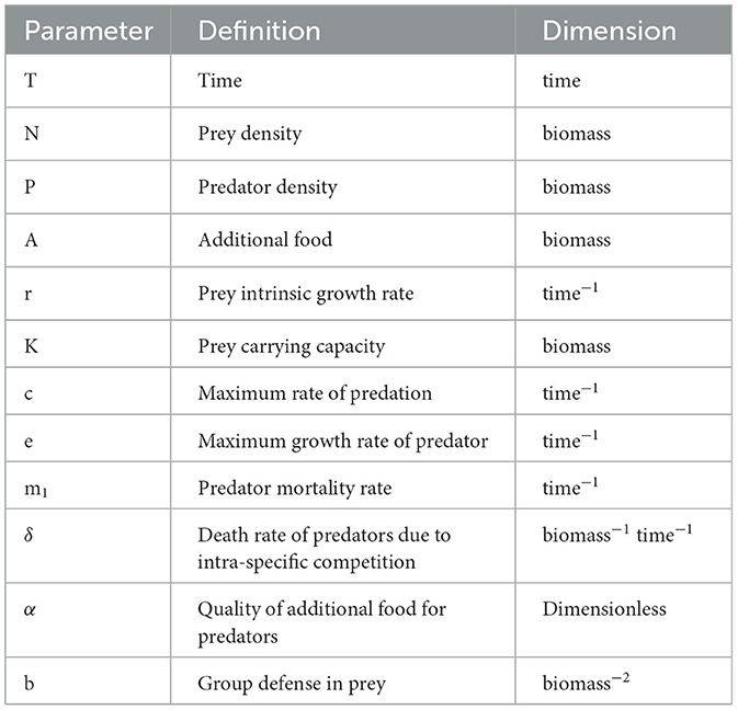
Table 1. Description of variables and parameters present in the systems (1), (2).

In order to reduce the complexity of the model, we non-dimensionalize the system (2) using the following non-dimensional parameters.

$N=ax,P=\frac{ay}{c},\gamma =\frac{K}{a},\xi =\frac{\eta A}{a},\omega =b{a}^2,m_2=\frac{c}{a\delta }.$

Accordingly, system (2) gets reduced to the following system.

$\begin{array}{ll}\begin{array}{l}\frac{\text{d}x}{\text{d}t}=rx\left(1-\frac{x}{\gamma }\right)-\left(\frac{xy}{(1+\alpha \xi )(\omega x^2+1)+x}\right)\\ \frac{\text{d}y}{\text{d}t}=e\left(\frac{x+\xi (\omega x^2+1)}{(\alpha \xi +1)(\omega x^2+1)+x}\right)y-m_{1}y-m_2{y}^2\end{array}& (3)\end{array}$

Here the term $\frac{\eta A^2}{N}$ denotes the quantity of additional food perceptible to the predator with respect to the prey relative to the nutritional value of prey to the additional food. Hence the term $\xi =\frac{\eta A}{a}$ can be seen to be an equivalent of quantity of additional food.

In real world scenarios, environmental fluctuations affect the dynamics of the system. In order to capture these fluctuations, we introduce the multiplicative white noise terms into (3). As in Sengupta et al., Bodine and Yust, and Srinivasu et al. [27, 29, 30], we now suppose that the intrinsic growth rate of prey and the death rate of predator are mainly affected by environmental noise such that

$r\to r+{\sigma }_{1}d{W}_1(t),m_1\to m_1+{\sigma }_{2}d{W}_2(t)$

where W_i(t) (i = 1, 2) are the mutually independent standard Brownian motions with W_i(0) = 0 and σ₁ and σ₂ are positive constants and they represent the intensities of the white noise.

Also, the system can go through huge, occasionally catastrophic disturbances. Since white noise is a continuous noise, it cannot capture sudden environmental changes. To cater to these, we also apply a discontinuous stochastic process as Lévy jumps to model these abrupt natural phenomenon as in Ma et al. and La Cognata et al. [24, 31].

We now perturb r and m₁ with discontinuous Lévy noise in addition to the continuous white noise. So, we have

$\begin{array}{l}r\to r+{\sigma }_1\text{d}{W}_1(t)+{\displaystyle {\int }_{𝕐}}{\gamma }_1(v)\tilde{N}(\text{d}t,\text{d}v),-m_1\\ \to -m_1+{\sigma }_2\text{d}{W}_2(t)+{\displaystyle {\int }_{𝕐}}{\gamma }_2(v)\tilde{N}(\text{d}t,\text{d}v)& (4)\end{array}$

According to the Lévy decomposition theorem [32], we have $\tilde{N}(t,dv)=N(t,dv)-\lambda (dv)t$, where $\tilde{N}(t,dv)$ is a compensated Poisson process and N is a Poisson counting measure with characteristic measure λ on a measurable subset 𝕐 of (0, +∞) with λ(𝕐) < ∞. The distribution of Lévy jumps L_i(t) can be completely parameterized by (a_i, σ_i, λ) and satisfies the property of infinite divisibility.

Now, by incorporating noise induced parameters (4) into the reduced deterministic system of Equation (3), we get the following additional food provided stochastic prey-predator system exhibiting Holling type-IV functional response along with the environmental fluctuations captured using the white noise and Lévy noise.

$\begin{array}{ll}\begin{array}{l}\text{d}x(t)=x(t)\left[r\left(1-\frac{x(t)}{\gamma }\right)-\left(\frac{y(t)}{(1+\alpha \xi )(\omega x^2(t)+1)+x(t)}\right)\right]\text{d}t\\ +{\sigma }_{1}x(t)\text{d}{W}_1(t)+x(t){\displaystyle {\int }_{𝕐}}{\gamma }_1(v)\tilde{N}(\text{d}t,\text{d}v)\\ \text{d}y(t)=y(t)\left[e\left(\frac{x(t)+\xi (\omega x^2(t)+1)}{(1+\alpha \xi )(\omega x^2(t)+1)+x(t)}\right)-m_1-m_{2}y(t)\right]\text{d}t\\ +{\sigma }_{2}y(t)\text{d}{W}_2(t)+y(t){\displaystyle {\int }_{𝕐}}{\gamma }_2(v)\tilde{N}(\text{d}t,\text{d}v)\end{array}& (5)\end{array}$

2.2. Existence of global positive solution

In order to do the stochastic time optimal control studies for the system (5), we first prove that the system (5) has a unique global positive solution.

Theorem 1. For any given initial value $X(\theta )=(x(\theta ),y(\theta ))\in C(\left[-{\tau }_0,0\right],{ℝ}^{{+}^2})$, there exists a unique positive global solution ((x(t), y(t)) of system (5) on t ≥ 0.

Note: The above theorem for existence of solutions of (5) can be proved in similar lines to the proof in Ma et al. [24] using the Lyapunov method.

Proof. For any given initial value $(x(\theta ),y(\theta ))\in C(\left[-{\tau }_0,0\right],{ℝ}^{{+}^2})$, there is a unique positive (x(t), y(t)) ∈ ℝ⁺² for t ∈ [0, τ_e], where τ_e is the explosion time. Subsequently, we will show that τ_e = ∞, which yields that (x(t), y(t)) is the global solution.

Let m₀ ≥ 0 be sufficiently large so x(t) and y(t) lie within the interval [1/m₀, m₀]. For each m ≥ m₀, we define the stopping time:

$\begin{array}{ll}{\tau }_e=\text{inf}\left\{t\in [-\omega ,{\tau }_e):x\notin (\frac{1}{m_0},m_0),y\notin (\frac{1}{m_0},m_0)\right\}& (6)\end{array}$

Evidently, τ_e is strictly increasing when m → ∞. Let τ_∞ = lim_{m → ∞}τ_m; thus τ_∞ ≤ τ_m a.s. Else there exist pairs of constants T > 0, m₁ ≥ m₀ and 0 < ϵ < 1 such that P(τ_∞ ≤ T) ≥ ϵ, m ≥ m₁.

Let V(x, y) = x − 1 − lnx+y − 1 − lny be a C²-function.

Using Itô's formula, we get

$\begin{array}{l}\text{d}V=LV\text{d}t+{\sigma }_1(x-1)d{W}_1+{\sigma }_2(y-1)d{W}_2\end{array}$

where

$\begin{array}{l}LV=(x-1)\left[r\right(1-\frac{x(t)}{\gamma })-(\frac{y(t)}{(1+\alpha \xi )(\omega x^2(t)+1)+x(t)}\left)\right]\\ +(y-1)\left[e\right(\frac{x(t)+\xi (\omega x^2(t)+1)}{(1+\alpha \xi )(\omega x^2(t)+1)+x(t)})\\ -m_1-m_{2}y(t)]+\frac{{\sigma }_1^2}{2}+\frac{{\sigma }_2^2}{2}\\ =rx-r-\frac{r}{\gamma }{x}^2+\frac{r}{\gamma }x-\frac{xy}{(1+\alpha \xi )(\omega x^2+1)+x}\\ +\frac{y}{(1+\alpha \xi )(\omega x^2+1)+x}+\frac{exy}{(1+\alpha \xi )(\omega x^2+1)+x}\\ +\frac{e\xi \omega x^{2}y}{(1+\alpha \xi )(\omega x^2+1)+x}+\frac{e\xi y}{(1+\alpha \xi )(\omega x^2+1)+x}\\ -\frac{ex}{(1+\alpha \xi )(\omega x^2+1)+x}-\frac{e\xi \omega x^2}{(1+\alpha \xi )(\omega x^2+1)+x}\\ -\frac{e\xi }{(1+\alpha \xi )(\omega x^2+1)+x}-m_{1}y+m_1-m_2{y}^2+m_{2}y\\ +\frac{{\sigma }_1^2}{2}+\frac{{\sigma }_2^2}{2}\\ \le rx-\frac{r}{\gamma }{x}^2+\frac{r}{\gamma }x+y\\ +ey+\frac{\xi e\omega }{\omega (1+\alpha \xi )}y+e\xi y\\ +m_1-m_2{y}^2+m_{2}y+\frac{{\sigma }_1^2}{2}+\frac{{\sigma }_2^2}{2}\\ =\left[\left(r+\frac{r}{\gamma }\right)x-\frac{r}{\gamma }{x}^2\right]\\ +\left[\left(e+e\xi +m_2+\frac{\xi e}{1+\alpha \xi }\right)y-m_2{y}^2\right]\\ +\left(m_1+\frac{{\sigma }_1^2}{2}+\frac{{\sigma }_2^2}{2}\right),\end{array}$

From derivative test, we can see that $Ax-B{x}^2\le \frac{A^2}{4B}$, where A and B are constants. Therefore,

$\begin{array}{l}LV\le \frac{{(r+\frac{r}{\gamma })}^2}{4\frac{r}{\gamma }}+\frac{1}{4m_2}{(e+e\xi +m_2+\frac{\xi e}{1+\alpha \xi })}^2\hfill \\ +(m_1+\frac{{\sigma }_1^2}{2}+\frac{{\sigma }_2^2}{2})\le K,\hfill \end{array}$

where K is a positive constant.

Thus,

$\begin{array}{l}\text{d}V\le K\text{d}t+{\sigma }_1(x-a)d{W}_1+{\sigma }_2(y-b)d{W}_2\end{array}$

Taking expectation, yields

$\begin{array}{l}EV(x({\tau }_m\wedge T),y({\tau }_m\wedge T))\le V(x(0),y(0))+E{\displaystyle {\int }_0^{{\tau }_m\wedge T}}Kdt.\end{array}$

Setting Ω_m = {τ_m∧T, m≥m₀}, we obtain P(Ω_m) ≥ ϵ. For each ω ∈ Ω_m, there are x(τ_m, ω), y(τ_m, ω) equaling either m or 1/m such that

$\begin{array}{l}V(x(0),y(0))+KT\ge E\left[1_{{\Omega }_k(\omega )}V(x({\tau }_m,\omega ),y({\tau }_m,\omega ))\right]\\ \ge ϵ\left[(\frac{1}{m}-1-\text{ln}\frac{1}{m})\wedge (m-1-\text{ln}m)\right],\end{array}$

where 1_Ωk(ω) denotes the indicator function of Ω_k(ω).

For m → ∞, we have

$\begin{array}{l}\infty >V(x(0),y(0))+KT=\infty \end{array}$

which is a contradiction. So, we have that τ_∞ = ∞. This completes the proof.□

2.3. Stochastic sensitivity analysis

In this subsection we briefly depict the sensitivity analysis for the remaining parameters that are not perturbed by noise. This can in turn help in understanding the sensitivity of the model with respect to these unperturbed parameters.

Figures 1–3 depict the local sensitivity of the stochastic model (5) w.r.t. the unperturbed parameters γ, ω, and e in the model.

FIGURE 1

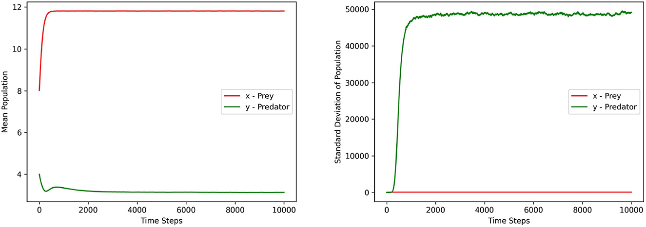
Figure 1. This figure depicts the mean and standard deviation of the predator, prey populations for the system (5) with respect to the parameter γ ∈ (10.1, 15.2). The values for other parameters are chosen as r = 1.5, ω = 15, α = 10, ξ = 0.10, e = 0.4, m₁ = 0.15, m₂ = 0.01, σ₁ = σ₂ = 0.2, γ₁ = γ₂ = 0.1.

FIGURE 2

Figure 2. This figure depicts the mean and standard deviation of the predator, prey populations for the system (5) with respect to the parameter ω ∈ (8.1, 15.2). The values for other parameters are chosen as r = 1.5, γ = 12, α = 10, ξ = 0.10, e = 0.4, m₁ = 0.15, m₂ = 0.01, σ₁ = σ₂ = 0.2, γ₁ = γ₂ = 0.1.

FIGURE 3

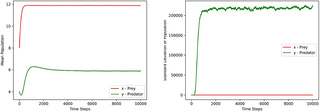
Figure 3. This figure depicts the mean and standard deviation of the predator, prey populations for the system (5) with respect to the parameter e ∈ (0.1, 0.9). The values for other parameters are chosen as r = 1.5, γ = 12, ω = 15, α = 10, ξ = 0.10, m₁ = 0.15, m₂ = 0.01, σ₁ = σ₂ = 0.2, γ₁ = γ₂ = 0.1.

In this local sensitivity analysis, we simulated the system (5) 1, 000 times for each value in the chosen parameter range.

Each figure contains two sub plots where the first and second plot depict the mean and standard deviation of prey, predator populations for the range of chosen parameter values respectively.

From the plots in Figures 1–3, it can be seen that the prey population in the system (5) is more sensitive with respect to these parameters than the predator population.

3. Stochastic time-optimal control problems

In this section, we formulate and study the stochastic time-optimal control problem for the prey-predator system (5) with quality (α) and quantity (ξ) of additional food as control variables.

3.1. Quality of additional food as stochastic time optimal control

In this subsection, we characterize the optimal quality of additional food for driving the system (5) to a desired equilibrium state in minimum time using the stochastic maximum principle. We fix the quantity of additional food ξ > 0 to be a constant and choose the objective functional to be minimized for this stochastic time optimal control problem as follows.

$\begin{array}{ll}J(\alpha )=E\left[{\displaystyle {\int }_0^T}1dt\right].& (7)\end{array}$

From the Sufficient Stochastic Maximum Principle [33] for the optimal control problems of jump diffusion, we characterize the optimal solution of the stochastic time optimal control problem with state space as the solutions of (5) and the objective functional (7).

Let (p^*, q^*, r^*) be a solution of the adjoint equation in the unknown processes p(t) ∈ ℝ², q(t) ∈ ℝ^{2 × 2}, r(t, z) ∈ ℝ² satisfying the backward differential equations

$\begin{array}{l}d{p}_1(t)=[\left(-r+\frac{2rx}{\gamma }-\frac{2\omega (1+\alpha \xi )x+1}{{((1+\alpha \xi )(\omega x^2+1)+x)}^2}\right)p_1(t)\\ -\frac{(1-\omega x^2)(1+(\alpha -1)\xi )}{{((1+\alpha \xi )(\omega x^2+1)+x)}^2}ey{p}_2(t)-{\sigma }_1{q}_1\\ -{\displaystyle \int {\gamma }_1}(v)r_1{v}_1(d{z}_1)]dt\\ +q_1(t)d{W}_1(t)+q_2(t)d{W}_2(t)+{\displaystyle {\int }_{{ℝ}^n}{r}_1\tilde{N}(dt,dz)}\\ d{p}_2(t)=-[\frac{-x}{(1+\alpha \xi )(\omega x^2+1)+x}{p}_1(t)\\ +\left(\frac{e(x+\xi (\omega x^2+1))}{(1+\alpha \xi )(\omega x^2+1)+x}-m_1-2m_{2}y\right)p_2(t)\\ +{\sigma }_2{q}_4+{\displaystyle \int {\gamma }_2}(v)r_2{v}_2(d{z}_2)]dt\\ +q_3(t)d{W}_1(t)+q_4(t)d{W}_2(t)+{\displaystyle {\int }_{{ℝ}^n}{r}_2\tilde{N}(dt,dz)}\\ p_1(T)=0,p_2(T)=0& (8)\end{array}$

The Hamiltonian associated with this control problem is defined as follows.

$\begin{array}{ll}\begin{array}{l}H(t,x,y,\alpha ,p,q,r)\\ =1+\left[r(1-\frac{x}{\gamma })-\frac{y}{(1+\alpha \xi )(1+\omega x^2)+x}\right]x{p}_1\\ +\left[\frac{e(x+\xi (\omega x^2+1))}{(1+\alpha \xi )(1+\omega x^2)+x}-m_1-m_{2}y\right]y{p}_2\\ +{\sigma }_{1}x{q}_1+{\sigma }_{2}y{q}_4+x\int {\gamma }_1{r}_1{v}_1(d{z}_1)+y\int {\gamma }_2(v)r_2{v}_2(d{z}_2)\end{array}& (9)\end{array}$

Let U = {α(t)|0 ≤ α(t) ≤ α_max∀t ∈ (0, t_f]} where ${\alpha }_{max}\in {ℝ}^{+}.$ Let α^*∈U with the corresponding solution (x^*, y^*) = [x(u^*), y(u^*)].

From the Arrow condition in the sufficient stochastic maximum Principle [33], we have

$\begin{array}{l}\frac{\partial H}{\partial \alpha }{|}_{{\alpha }^{*}}=0\\ \Rightarrow [-yx{p}_1\frac{-\xi (\omega x^2+1}{{((1+\alpha \xi )(\omega x^2+1)+x)}^2}\\ -\frac{ey{p}_2(x+\xi (\omega x^2+1))(\xi (\omega x^2+1))}{{((1+\alpha \xi )(\omega x^2+1)+x)}^2}]{|}_{*}=0\\ \Rightarrow [yx{p}_1-ey{p}_2(x+\xi (\omega x^2+1))]{|}_{*}=0\\ \Rightarrow x^{*}{p}_1^{*}=e{p}_2^{*}(x^{*}+\xi (\omega x^{{*}^2}+1))\end{array}$

Hence the optimal control α^* should satisfy the following condition.

$\begin{array}{ll}{x}^{*}{p}_1^{*}=e{p}_2^{*}(x^{*}+\xi (\omega x^{{*}^2}+1))& (10)\end{array}$

Since the analytical solution of (8) is complex to solve, we numerically simulate these results in Subsection 3.4.

3.2. Quantity of additional food as stochastic time optimal control

In this subsection, we characterize the optimal quantity of additional food for driving the system (5) to a desired equilibrium state in minimum time using the stochastic maximum principle. We fix the quality of additional food α > 0 to be a constant and choose the objective functional to be minimized for this stochastic time optimal control problem as follows.

$\begin{array}{ll}J(\xi )=E\left[{\displaystyle {\int }_0^T}1dt\right].& (11)\end{array}$

From the Sufficient Stochastic Maximum Principle [33] for the optimal control problems of jump diffusion, we characterize the optimal solution of the stochastic time optimal control problem with state space as the solutions of (5) and the objective functional (11).

Let (p^*, q^*, r^*) be a solution of the adjoint equation in the unknown processes p(t) ∈ ℝ², q(t) ∈ ℝ^{2 × 2}, r(t, z) ∈ ℝ² satisfying the backward differential equations

$\begin{array}{l}d{p}_1(t)=[(-r+\frac{2rx}{\gamma }-\frac{2\omega (1+\alpha \xi )x+1}{{((1+\alpha \xi )(\omega x^2+1)+x)}^2})p_1(t)\\ -\frac{(1-\omega x^2)(1+(\alpha -1)\xi )}{{((1+\alpha \xi )(\omega x^2+1)+x)}^2}ey{p}_2(t)\\ -{\sigma }_1{q}_1-{{\displaystyle \int }}^{\text{}}{\gamma }_1(v)r_1{v}_1(d{z}_1)]dt\\ +q_1(t)d{W}_1(t)+q_2(t)d{W}_2(t)+{\displaystyle {\int }_{{ℝ}^n}{r}_1\tilde{N}(dt,dz)}\\ d{p}_2(t)=-[\frac{-x}{(1+\alpha \xi )(\omega x^2+1)+x}{p}_1(t)\\ +(\frac{e(x+\xi (\omega x^2+1))}{(1+\alpha \xi )(\omega x^2+1)+x}-m_1-2m_{2}y)p_2(t)+{\sigma }_2{q}_4\\ +{{\displaystyle \int }}^{\text{}}{\gamma }_2(v)r_2{v}_2(d{z}_2)]dt+q_3(t)d{W}_1(t)\\ +q_4(t)d{W}_2(t)+{\displaystyle {\int }_{{ℝ}^n}{r}_2\tilde{N}(dt,dz)}\\ p_1(T)=0, p_2(T)=0& (12)\end{array}$

The Hamiltonian associated with this control problem is defined as follows.

$\begin{array}{ll}\begin{array}{l}H(t,x,y,\xi ,p,q,r)\\ =1+\left[r(1-\frac{x}{\gamma })-\frac{y}{(1+\alpha \xi )(1+\omega x^2)+x}\right]x{p}_1\\ +\left[\frac{e(x+\xi (\omega x^2+1))}{(1+\alpha \xi )(1+\omega x^2)+x}-m_1-m_{2}y\right]y{p}_2\\ +{\sigma }_{1}x{q}_1+{\sigma }_{2}y{q}_4+x\int {\gamma }_1{r}_1{v}_1(d{z}_1)+y\int {\gamma }_2(v)r_2{v}_2(d{z}_2)\end{array}& (13)\end{array}$

Let U = {ξ(t)|0 ≤ ξ(t) ≤ ξ_max∀t ∈ (0, t_f]} where ${\xi }_{max}\in {ℝ}^{+}.$ Let ξ^*∈U with the corresponding solution (x^*, y^*) = (x(ξ^*), y(ξ^*)).

From the Arrow condition in the sufficient stochastic maximum Principle [33], we have

$\begin{array}{l}\frac{\partial H}{\partial \xi }{|}_{{\xi }^{*}}=0\\ \Rightarrow [-yx{p}_1\frac{-\alpha (\omega x^2+1}{{((1+\alpha \xi )(\omega x^2+1)+x)}^2}+\\ ey{p}_2\left(\frac{((1+\alpha \xi )(\omega x^2+1)+x)(\omega x^2+1)-\alpha (\omega x^2+1)(x+\xi (\omega x^2+1))}{{((1+\alpha \xi )(\omega x^2+1)+x)}^2}\right)]{|}_{*}=0\\ \Rightarrow [\alpha xy(\omega x^2+1)p_1+ey{p}_2(\omega x^2+1)(x(1-\alpha )(\omega x^2+1))]{|}_{*}=0\\ \Rightarrow [\alpha x{p}_1+e{p}_2(1+\omega x^2+x(1-\alpha ))]{|}_{*}=0\\ \Rightarrow \alpha x^{*}{p}_1^{*}+e{p}_2^{*}(1+\omega x^{{*}^2}+x^{*}(1-\alpha ))=0\end{array}$

Hence the optimal control ξ^* should satisfy the following condition.

$\begin{array}{ll}\alpha x^{*}{p}_1^{*}+e{p}_2^{*}(1+\omega x^{{*}^2}+x^{*}(1-\alpha ))=0& (14)\end{array}$

Since the analytical solution of (8) is complex to solve, we numerically simulate these results in Subsection 3.4.

3.3. Existence and uniqueness of solutions for the Forward Backward Stochastic Differential Equations with Jumps (FBSDEJ)

We so far obtained the adjoint Equations 8, 12 for the state Equation 5 and the objective functional (7), (11) using the sufficient stochastic maximum principle respectively. Upon simplifying the results obtained from the arrow condition (10), (14) from earlier two subsections, we see that the optimal controls are given by

$\begin{array}{ll}{\alpha }^{*}=\frac{e{p}_2^{*}(1+x^{*}+\omega x^{{*}^2})}{e{p}_2^{*}{x}^{*}-p_1^{*}{x}^{*}},{\xi }^{*}=\frac{x^{*}{p}_1^{*}-e{x}^{*}{p}_2^{*}}{e{p}_2^{*}(1+\omega x^{{*}^2})}& (15)\end{array}$

In this section, we now prove the existence of optimal controls by proving the existence of the solutions for the FBSDEJ [(5), (8), (12)] which establishes the existence of $(x^{*},y^{*},p_1^{*},p_2^{*})$ for all simulation purposes. Using the theorem in Al-Hussein and Gherbal [34], we now prove the existence of the optimal controls (15) in the following theorem.

Theorem 2. For any $(x_0,y_0)\in {ℝ}^{{+}^2}$, the FBSDEJ [(5), (8), (12)] admits an optimal stochastic control.

Proof. Let (_Xt)t≥0 be the solution of the Stochastic Differential Equation with Jumps (SDEJ)

$\begin{array}{l}\text{d}{X}_t=b(X_t)dt+\sigma (X_t)dW(t)+{\displaystyle {\int }_{ℝ}\Gamma (v)\tilde{N}(dt,dv)}\hfill \end{array}$

Here the term b(X_t) denotes the drift coefficient, the term σ(X_t) denotes the diffusion coefficient and the term Γ(v) denotes the poisson term coefficient.

The theorem 1 in Section 3 guaranties the monotonicity and Lipschitz continuity of the drift coefficient, the diffusion coefficient and the poisson term coefficient of the state Equation 5.

Following the the existence and uniqueness theorem of FBDSDEJ in Al-Hussein and Gherbal [34], we are only left to prove the monotonicity and Lipschitz continuity of the drift and diffusion terms of the adjoint system of Equation 8.

From (8), due to the positivity of state variables guaranteed by theorem 1, the drift term and the diffusion terms are given as follows.

$\begin{array}{l}b(X_t)\le \left(\begin{array}{c}(\frac{2rx}{\gamma })p_1(t)+(\omega e{x}^{2}y)p_2(t)\\ (x)p_1(t)+(m_1+2m_{2}y)p_2(t)\end{array}\right),\sigma (X_t)=\left(\begin{array}{c}{q}_1(t)q_2(t)\\ q_3(t)q_4(t)\end{array}\right)\end{array}$

Since the drift coefficient is a linear combination of adjoint terms (p₁, p₂), the monotonicity and Lipschitz continuity are guaranteed.

In addition to this, the diffusion coefficient is independent of the adjoint terms (p₁, p₂). Therefore, the monotonicity and Lipschitz continuity are guaranteed for the diffusion coefficients.

Hence the existence of unique stochastic optimal controls are proved for FBSDEJ [(5), (8), (12)].□

3.4. Numerical simulations

In this section, we perform the extensive numerical simulations using python by choosing the following parameters [24] for the model (5). r = 1.5, γ = 12, ω = 15, e = 0.4, m₁ = 0.15, m₂ = 0.01, σ₁ = σ₂ = 0.02, γ₁ = 1, γ₂ = 1. In these simulations, white noise is simulated using the Box-Normal transformations and the poisson noise is simulated using the poisson point processes [35]. The state Equation 5 and the adjoint Equations 8, 12 are simulated using the Forward Backward Doubly Stochastic Differential Equations with Jumps (FBDSDEJ) method. The subplots in Figures 4, 5 depict the optimal state trajectories, optimal co-state trajectories, phase diagram, optimal quality of additional food and the optimal quantity of additional food respectively.

FIGURE 4

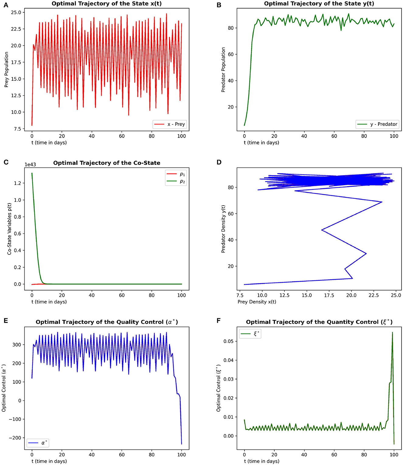
Figure 4. This figure depicts the simulations of time-optimal control problem with respect to the control variables in the context of biological conservation. The subfigures (A–C) depict the optimal prey, predator and co-state vectors respectively. The subfigure (D) depicts the phase diagram between prey and predator densities. The subfigures (E, F) depict the optimal quality and quantity control variables. The parameter values are chosen as r = 1.5, γ = 12, ω = 15, e = 0.4, m₁ = 0.15, m₂ = 0.01.

FIGURE 5

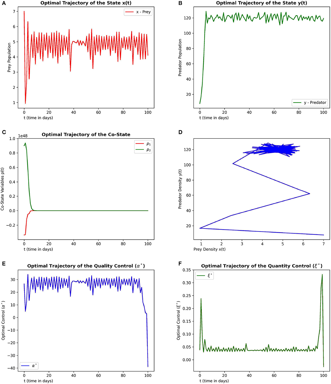
Figure 5. This figure depicts the simulations of time-optimal control problem with respect to the control variables in the context of pest management. The subfigures (A–C) depict the optimal prey, predator and co-state vectors respectively. The subfigure (D) depicts the phase diagram between prey and predator densities. The subfigures (E, F) depict the optimal quality and quantity control variables. The parameter values are chosen as r = 1.5, γ = 4, ω = 6, e = 0.6, m₁ = 0.1, m₂ = 0.01.

3.4.1. Applications to biological conservation

The subplots (4a) and (4b) depicts the optimal state trajectory of the system (5) from the initial state (2, 8) that stabilizes over time around the state (16, 90). The subplot (4d) gives the phase diagram which shows the trajectories are stabilized over high values of prey and predator. The subplots (4e) and (4f) depicts the optimal quality and quantity of additional food respectively. These plots show that the high quality of additional food is required to achieve biological conservation. Even if the quantity of additional food is lower, still we will be able to achieve biological conservation with higher quality of additional food.

3.4.2. Applications to pest management

The subplots (5a) and (5b) depicts the optimal state trajectory of the system (5) from the initial state (7, 5). It can be seen that the system can be driven to a low prey dominated state. The subplot (5d) depicts this property more clearly through the phase diagram where it reaches the lowest prey value over the time. The subplots (5e) and (5f) depicts that a lesser quality of additional food and a lower quantity of additional food is good enough to achieve pest management where pest is viewed as prey.

3.5. Sensitivity of time optimal controls

In this subsection we perform the sensitivity analysis for the optimal control variables α(t) and ξ(t) with respect to the different values for the model parameters

In Figure 6, frames (6a) and (6b) depict the sensitivity of the control variables with respect to the parameters r and γ respectively. Frames (6c) and (6d) depict the sensitivity of the control variables with respect to the parameters ω and e respectively. In Figure 6, frames (6a) and (6b) depict the sensitivity of the control variables with respect to the parameters m₁ and m₂, respectively.

FIGURE 6

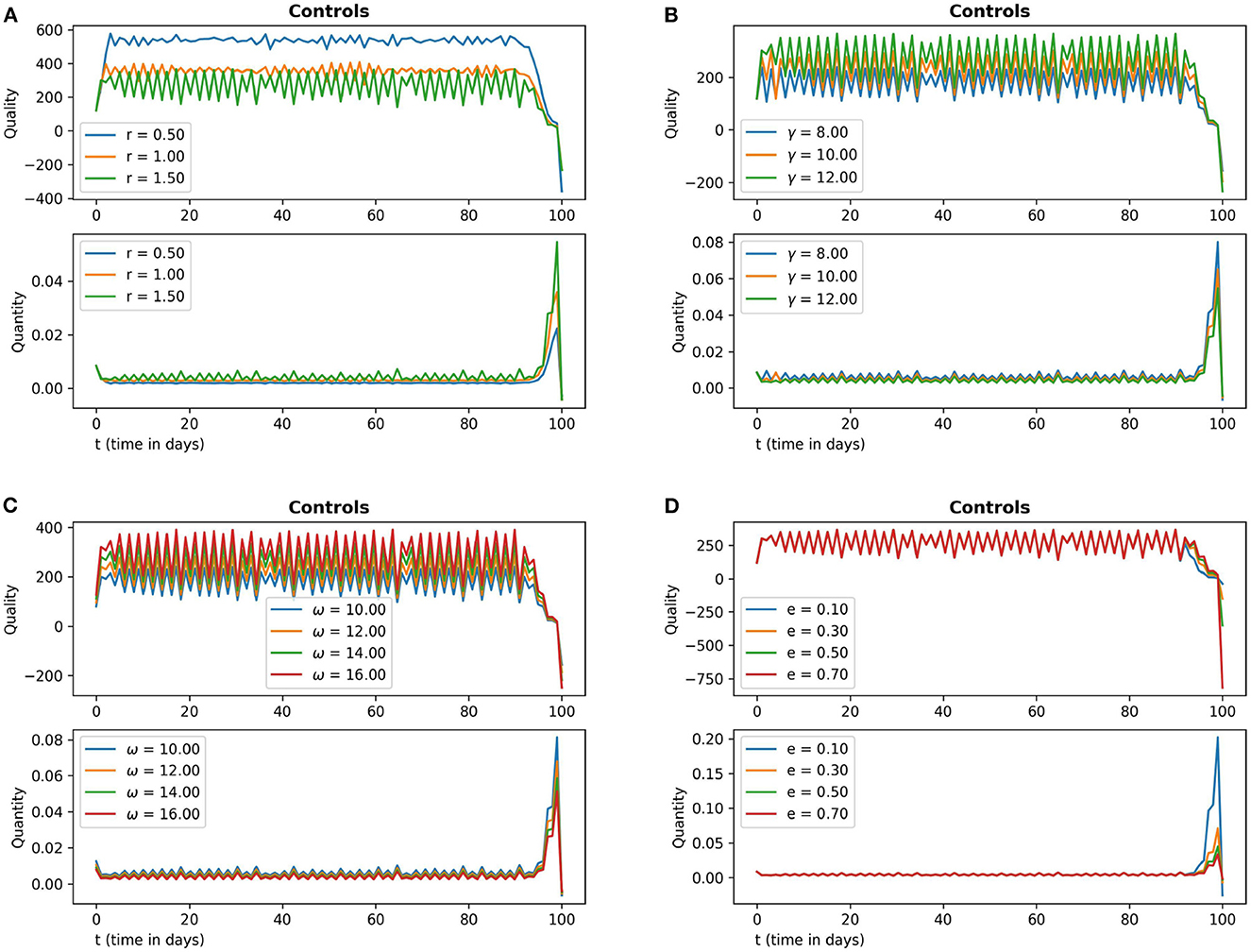
Figure 6. The subfigures (A–D) in this figure depict the optimal quality and optimal quantity of additional food (15) with respect to the parameter values r, γ, ω and e respectively. The other parameter values are chosen as r = 1.5, γ = 12, ω = 15, e = 0.4, m₁ = 0.15, m₂ = 0.01.

From the sensitivity analysis depicted in Figures 6, 7 we see that the optimal quality control seems to be more sensitive with respect to the parameter r in comparison to the other parameters.

FIGURE 7

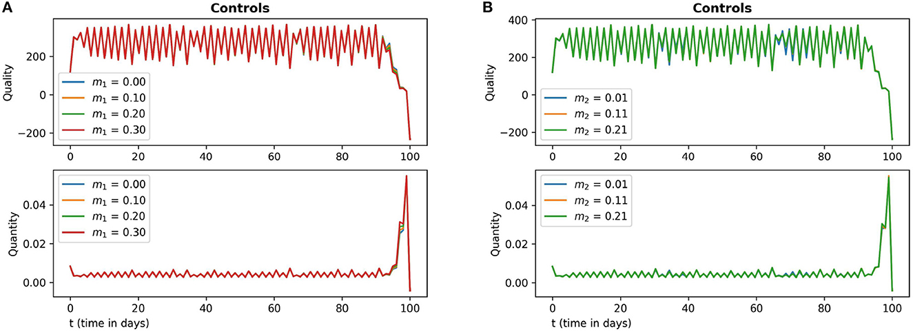
Figure 7. The subfigures (A, B) in this figure depict the optimal quality and optimal quantity of additional food (15) with respect to the parameter values m₁ and m₂ respectively. The other parameter values are chosen as r = 1.5, γ = 12, ω = 15, e = 0.4.

4. Effect of noise on the optimal control problem

In this section, we briefly study the effects of discrete and continuous noise on the system (3). We compared the dynamics of the state trajectories and control variables with and without these noises.

In Figure 8, frames (8a) and (8b) depict the optimal prey and optimal predator populations respectively with no noise, white noise and with both white noise and Lévy noise. Frame (8c) depicts the corresponding trajectories of co-state variables. Frame (8d) depicts the phase space of the state variables. Frames (8e) and (8f) depict the optimal quality and quantity control trajectories respectively.

FIGURE 8

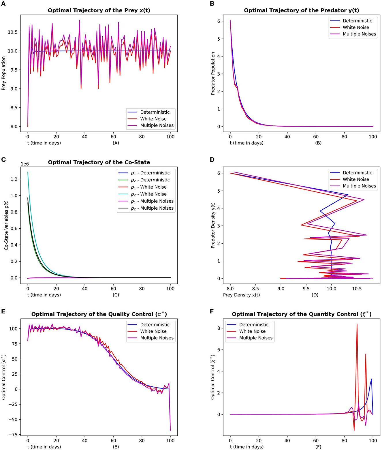
Figure 8. This figure depicts the simulations of time-optimal control problem with respect to the control variables. The subfigures (A–C) depict the optimal prey, predator and co-state vectors respectively. The subfigure (D) depicts the phase diagram between prey and predator densities. The subfigures (E, F) depict the optimal quality and quantity control variables. The three graphs in each subfigure corresponds to the dynamics of the system with no noise, white noise and multiple noises. The parameter values are chosen as r = 1.5, γ = 12, ω = 15, e = 0.4, m₁ = 0.15, m₂ = 0.01.

From the plots in Figure 8 we see that both the discrete and continuous noise can lead to fluctuations in prey dynamics compared to that of predator. From the phase plots it can be seen that the converging pattern to the final state more or less follow a similar trend. Overall we find that the prey seems to be more influenced by the noise than that of predator.

5. Discussions and conclusions

This paper studies a stochastic prey-predator system exhibiting Holling type-IV functional response along with the combined influence of white noise and Lévy noise. We do the time-optimal control studies for this system, with the quality and the quantity of additional food as control variables. To begin with, we formulated a stochastic model by considering multiplicative noise to both prey and predator. In theorem 1, we proved the existence of a unique positive global solution of (5). Further, we formulated the time-optimal control problem with the objective to minimize the final time in which the system reaches the pre-defined state. Using the sufficient stochastic maximum principle, we characterized the optimal control values. In theorem 2, we proved that the existence and uniqueness of Forward Backward Doubly Stochastic Differential Equations with Jumps (FBDSDEJ). We also numerically simulated the theoretical findings and applied them in the context of biological conservation and pest management.

To understand the sensitivity of this stochastic system, we firstly performed the sensitivity analysis with respect to the individual parameters and later did the sensitivity analysis for the optimal control variables with respect to the parameters of the system. The findings revealed that the stochastic system as such is minimally sensitive with respect to the system parameters and the optimal quality control variable seems to be more sensitive with respect to the parameter, growth rate r relative to the other parameters.

Finally a brief study on the influence of different noises on this stochastic system revealed that both the discrete and continuous noise induced fluctuations in the prey dynamics and seem to have minimal effect on the predator dynamics.

Some of the salient features of this work include the following. Unlike the most traditional papers, here we considered a stochastic time-optimal control problem. As Intra-specific competition among predators is ineluctable, we also explicitly incorporated the intra-specific competition into our model. This paper mainly deals with the novel study of the time-optimal control problems where the state equations involve both the discrete and continuous noise which is challenging. We also performed the stochastic sensitivity analysis.

To sum up this work has been an initial attempt and a first of its kind dealing with the Stochastic Time Optimal Control studies for prey-predator systems involving group defense of the prey. Since this is an initial exploratory research we didn't include finer specificalities such as mutual interference of the predators and also did not elaborate much on the stochastic bifurcation aspect. In future we wish to incorporate and study these aspects. We also intend to extend these studies in the setting of Markov Chain and Partial Differential Equations.

Data availability statement

The original contributions presented in the study are included in the article/supplementary material, further inquiries can be directed to the corresponding author.

Author contributions

DP conceived the idea, worked and executed all the theoretical and numerical findings, and framed the manuscript. DV conceived and designed the paper, helped in structuring, and finalizing the manuscript. All authors contributed to the article and approved the submitted version.

Funding

This research was supported by National Board of Higher Mathematics (NBHM), Department of Atomic Energy (DAE), Government of India under project grant-Time Optimal Control Studies and Bifurcation Analysis of Coupled Nonlinear Dynamical Systems with Applications to Pest Management, Sanction number: [02011/11/2021NBHM(R.P)/R&D II/10074].

Acknowledgments

The authors dedicate this paper to the founder chancellor of SSSIHL, Bhagawan Sri Sathya Sai Baba. DV also dedicates this paper to his loving elder brother D. A. C. Prakash who still lives in his heart.

Conflict of interest

The authors declare that the research was conducted in the absence of any commercial or financial relationships that could be construed as a potential conflict of interest.

Publisher's note

All claims expressed in this article are solely those of the authors and do not necessarily represent those of their affiliated organizations, or those of the publisher, the editors and the reviewers. Any product that may be evaluated in this article, or claim that may be made by its manufacturer, is not guaranteed or endorsed by the publisher.

References

1. Lotka AJ. Elements of Physical Biology. Philadelphia, PA: Williams & Wilkins (1925).

Google Scholar

2. Volterra V. Variazioni e fluttuazioni del numero d'individui in specie animali conviventi. Memoria della Reale Accademia Nazionale dei Lincei. (1927) 2:31–113.

Google Scholar

3. Kot M. Elements of Mathematical Ecology. Cambridge: Cambridge University Press (2001).

Google Scholar

4. Metz JA, Diekmann O. The Dynamics of Physiologically Structured Populations. Cham: Springer (2014). vol. 68.

Google Scholar

5. Geritz S, Gyllenberg M. A mechanistic derivation of the DeAngelis–Beddington functional response. J Theoret Biol. (2012) 314:106–8. doi: 10.1016/j.jtbi.2012.08.030

PubMed Abstract | CrossRef Full Text | Google Scholar

6. Arditi R, Ginzburg LR. Coupling in predator-prey dynamics: ratio-dependence. J Theoret Biol. (1989) 139:311–26.

Google Scholar

7. Hassell M, Varley G. New inductive population model for insect parasites and its bearing on biological control. Nature. (1969) 223:1133–7.

PubMed Abstract | Google Scholar

8. Crowley PH, Martin EK. Functional responses and interference within and between year classes of a dragonfly population. J North Am Benthol Soc. (1989) 8:211–21.

PubMed Abstract | Google Scholar

9. Freedman HI, Wolkowicz GS. Predator-prey systems with group defence: the paradox of enrichment revisited. Bullet Math Biol. (1986) 48:493–508.

PubMed Abstract | Google Scholar

10. Yano S. Cooperative web sharing against predators promotes group living in spider mites. Behav Ecol Sociobiol. (2012) 66:845–53. doi: 10.1007/s00265-012-1332-5

CrossRef Full Text | Google Scholar

11. McClure M, Despland E. Defensive responses by a social caterpillar are tailored to different predators and change with larval instar and group size. Naturwissenschaften. (2011) 98:425–34. doi: 10.1007/s00114-011-0788-x

PubMed Abstract | CrossRef Full Text | Google Scholar

12. Srinivasu PDN, Prasad BSRV, Venkatesulu M. Biological control through provision of additional food to predators: a theoretical study. Theoret Popul Biol. (2007) 72:111–20. doi: 10.1016/j.tpb.2007.03.011

PubMed Abstract | CrossRef Full Text | Google Scholar

13. Srinivasu PDN, Prasad BSRV. Time optimal control of an additional food provided predator–prey system with applications to pest management and biological conservation. J Math Biol. (2010) 60:591–613. doi: 10.1007/s00285-009-0279-2

PubMed Abstract | CrossRef Full Text | Google Scholar

14. Srinivasu PDN, Vamsi DKK, Aditya I. Biological conservation of living systems by providing additional food supplements in the presence of inhibitory effect: a theoretical study using predator–prey models. Diff Eq Dyn Syst. (2018) 26:213–46. doi: 10.1007/s12591-016-0344-4

CrossRef Full Text | Google Scholar

15. Srinivasu PDN, Vamsi DKK, Ananth VS. Additional food supplements as a tool for biological conservation of predator-prey systems involving type III functional response: a qualitative and quantitative investigation. J Theoret Biol. (2018) 455:303–18. doi: 10.1016/j.jtbi.2018.07.019

PubMed Abstract | CrossRef Full Text | Google Scholar

16. Vamsi DKK, Kanumoori DSSM, Chhetri B. Additional food supplements as a tool for biological conservation of biosystems in the presence of inhibitory effect of the prey. Acta Biotheoret. (2020) 68:321–55. doi: 10.1007/s10441-019-09371-x

PubMed Abstract | CrossRef Full Text | Google Scholar

17. Ananth VS, Vamsi DKK. An optimal control study with quantity of additional food as control in prey-predator systems involving inhibitory effect. Comput Math Biophys. (2021) 9:114–45. doi: 10.1515/cmb-2020-0121

PubMed Abstract | CrossRef Full Text | Google Scholar

18. Sabelis MW, Van Rijn PC. When does alternative food promote biological pest control? IOBC WPRS Bulletin. (2006) 29:195. Available online at: https://bugwoodcloud.org/bugwood/anthropod/2005/vol2/8e.pdf

Google Scholar

19. Ananth VS, Vamsi DKK. Achieving minimum-time biological conservation and pest management for additional food provided predator–Prey systems involving inhibitory effect: a qualitative investigation. Acta Biotheoret. (2022) 70:1–51. doi: 10.1007/s10441-021-09430-2

PubMed Abstract | CrossRef Full Text | Google Scholar

20. May RM. Stability and complexity in model ecosystems. In: Stability and Complexity in Model Ecosystems. Princeton, NJ: Princeton University Press (2019) 109–138.

Google Scholar

21. Elton CS. The Ecology of Invasions by Animals and Plants. Berlin: Springer Nature (2020).

Google Scholar

22. Li L, Zhao W. Deterministic and stochastic dynamics of a modified Leslie-Gower prey-predator system with simplified Holling-type IV scheme. Math Biosci Eng. (2021) 18:2813–31. doi: 10.3934/mbe.2021143

PubMed Abstract | CrossRef Full Text | Google Scholar

23. Xu D, Liu M, Xu X. Analysis of a stochastic predator–prey system with modified Leslie–Gower and Holling-type IV schemes. Phys A Stat Mech Appl. (2020) 537:122761. doi: 10.1016/j.physa.2019.122761

CrossRef Full Text | Google Scholar

24. Ma T, Meng X, Chang Z. Dynamics and optimal harvesting control for a stochastic one-predator-two-prey time delay system with jumps. Complexity. (2019) 2019. doi: 10.1155/2019

CrossRef Full Text | Google Scholar

25. Jia W, Xu Y, Li D, Hu R. Stochastic analysis of predator–prey models under combined gaussian and poisson white noise via stochastic averaging method. Entropy. (2021) 23:1208. doi: 10.3390/e23091208

PubMed Abstract | CrossRef Full Text | Google Scholar

26. Prakash DB, Vamsi DKK. Stochastic optimal and time-optimal control studies for additional food provided prey–predator systems involving Holling type III functional response. Comput Math Biophys. (2023) 11:20220144. doi: 10.48550/arXiv.2207.06668

CrossRef Full Text | Google Scholar

27. Sengupta S, Das P, Mukherjee D. Stochastic non-autonomous Holling type-III prey-predator model with predator's intra-specific competition. Discr Contin Dyn Syst B. (2018) 23:3275. doi: 10.3934/dcdsb.2018244

CrossRef Full Text | Google Scholar

28. Bodine EN, Yust AE. Predator-prey dynamics with intraspecific competition and an allee effect in the predator population. Lett Biomathemat. (2017) 4:23–38. doi: 10.1080/23737867.2017.1282843

CrossRef Full Text | Google Scholar

29. Bera SP, Maiti A, Samanta G. Stochastic analysis of a prey–predator model with herd behaviour of prey. Nonlin Anal. (2016) 21:345–61. doi: 10.15388/NA.2016.3.4

CrossRef Full Text | Google Scholar

30. Belabbas M, Ouahab A, Souna F. Rich dynamics in a stochastic predator-prey model with protection zone for the prey and multiplicative noise applied on both species. Nonlin Dyn. (2021) 106:2761–80. doi: 10.1007/s11071-021-06903-4

CrossRef Full Text | Google Scholar

31. La Cognata A, Valenti D, Dubkov A, Spagnolo B. Dynamics of two competing species in the presence of Lévy noise sources. Phys Rev E. (2010) 82:e011121. doi: 10.1103/PhysRevE.82.011121

PubMed Abstract | CrossRef Full Text | Google Scholar

32. Øksendal B, Sulem A. Stochastic Control of Jump Diffusions. Cham: Springer (2005).

Google Scholar

33. Framstad NC, Øksendal B, Sulem A. Sufficient stochastic maximum principle for the optimal control of jump diffusions and applications to finance. J Opt Theory Appl. (2004) 121:77–98. doi: 10.1023/B:JOTA.0000026132.62934.96

CrossRef Full Text | Google Scholar

34. Al-Hussein A, Gherbal B. Existence and uniqueness of the solutions of forward-backward doubly stochastic differential equations with Poisson jumps. Random Operat Stochast Eq. (2020)28:253–68. doi: 10.1515/rose-2020-2044

CrossRef Full Text | Google Scholar

35. Zou X, Wang K. Numerical simulations and modeling for stochastic biological systems with jumps. Commun Nonlin Sci Numer Simulat. (2014) 19:1557–68. doi: 10.1016/j.cnsns.2013.09.010

CrossRef Full Text | Google Scholar