A Runge-Kutta numerical scheme applied in solving predator-prey fuzzy model with Holling type II functional response

The predator-prey model has been extensively studied, but only studies models in a certain environment, where all parameters and initial values involved in the model are assumed to be certain. In real practice, some parameters and initial values are often uncertain. To overcome this uncertainty problem, a model can be made by using a fuzzy theoretical approach. In this paper, we develop a numerical scheme for solving two predator-prey models with a Holling type II functional response by considering fuzzy parameters and initial populations. The behavior of the model was studied qualitatively using the 5th order Runge-Kutta method of which was modified for the fuzzy system using the Zadeh extension principle. The numerical simulation results show that, when the initial populations of prey and predators are fuzzy, the behavior of the fuzzy model would be qualitatively the same as the crisp model. Finally, we conclude that the resulting fuzzy behavior represents a generalization of crisp behavior. This gives more realistic results since the solution is obtained by explicitly considering the problem of uncertainty.

1. Introduction

The predator-prey model is a model of the interaction between two species expressed in the form of a system of differential equations that describes the dynamic relationship between prey and predators [1]. This model was first introduced by Lotka and Volterra, so it is known as the Lotka-Volterra predator-prey model. In this model, the dynamic behavior of a simple predator-prey model is studied. Various applications of the predator-prey system, such as those in Supriatna and Possingham [2, 3] and several other modifications of the predator-prey model have been made by incorporating additional biological processes into the classic Lotka-Volterra predator-prey equation, including functional response modifications [4].

In ecological systems, the degree of predation depends on the functional response. A functional response considers the number of prey that the predator has successfully consumed per unit time. It is also introduced to describe changes in the rate of prey consumption by predators when prey density varies [4]. The most common and well-known functional response is the type-II Holling functional response. The Holling type II functional response describes the increasing rate of predator's consumption when the density of prey is low. Meanwhile, when the prey density is high, the predator's consumption is constant. In this case, it represents a phenomenon that the predator takes very little time to find the prey, and when the prey consumption rate reaches the highest level, the predator becomes easily full.

In recent years, various studies on predator-prey models with type-II Holling functional responses have been carried out, including in in Dawes and Souze [4], Jana and Kar [5], Ma et al. [6]. Those studies consider a predator-prey model in a definite environment, where all parameters affecting population size and initial values involved in the model are assumed to be crisp. However, in reality, each parameter and initial value is uncertain, unclear, or incomplete. This uncertainty is caused by inaccuracies made during the process of observation, measurement, experimentation, and so on. To overcome this problem, a model can be made using different approaches such as the stochastic approach, the fuzzy approach and the fuzzy-stochastic approach. A crisp ODE system could be more suitable to be converted into a fuzzy differential equation system whenever the parameters or the initial values are uncertain and have a degree of perseptional values.

In recent decades, the application of fuzzy theory has been widely used as a very effective tool in mathematical modeling to solve real problems that take into account uncertainty. In this approach, uncertain variables and parameters are represented by intervals and fuzzy numbers. In the study of fuzzy differential equations, the term fuzzy differential equations can be in the form of differential equations with fuzzy coefficients, differential equations with fuzzy initial values or fuzzy boundary values [7–12]. The stability of the fuzzy dynamic system in a dynamic population is studied through fuzzy differential equation and fuzzy initial value problem [13]. Various numerical solutions for systems of fuzzy equations have also been introduced in Ahmad and Hasan [10], Jayakumar et al. [14], Nayak and Chakraverty [15], Behroozpoor et al. [16], Tapaswini and Chakraverty [17], and Tapaswini and Chakraverty [18].

The fuzzy predator-prey model was first introduced in da Silva Peixoto et al. [19], where a classic deterministic predator-prey model was formulated using a fuzzy rule-based system. The development of fuzzy differential equations has resulted in new discoveries of fuzzy predator-prey models, including those made by Ahmad and Hasan [10], Pandit and Singh [20], Ak and Oru [21], Ahmad and De Baets [22], Narayanamoorthy et al. [23], Omar et al. [24], and Pal et al. [25]. The authors in Ahmad and Hasan [10], Ahmad and De Baets [22], and Omar et al. [24] used the Euler and 4th order Runge-Kutta method through the principles of Zadeh extension. While the authors in Ak and Oru [21], used the concept of generalized fuzzy derivatives. Other authors in Pandit and Singh [20], used Hukuhara derivative. Moreover, the authors in Narayanamoorthy et al. [23], used the fractional modified Euler method. On the biological perspective, there are some authors who have studied fuzzy predator-prey models with functional responses such as [20, 23, 24, 26]. They all studied a predator-prey model with fuzzy initial conditions. Fuzzy predator-prey models with functional responses have also been studied by Pal et al. [27], Yu et al. [28], Pal et al. [29], Meng and Wu [30], Mahata et al. [31], and Pal et al. [32], who presented fuzzy predator-prey harvesting models. Their work studied two species of predator-prey harvesting models by considering fuzzy parameters. Among those work, the authors in Mallak et al. [26], studied a fuzzy predator-prey model with an arctan functional response using the Hukuhara derivative approach, to describe the satiation predator's consumption.

Our research discusses predator-prey models with Holling type II functional responses by considering fuzzy parameters and fuzzy initial populations. The motivation is that we would like to see how different is the dynamics of the sytems compared to their counterpart crisp predator-prey systems. To proceed we will present some preliminaries regarding the fuzzy number theory and fuzzy differential equation background in Sections 2 and 3 followed by the 5th order Runge-Kutta numerical scheme for fuzzy differential Section 4. In Section 5, we discuss the equilibria and their stabilities condition for two predator-prey models with fuzzy parameters and fuzzy initial values followed by the applications of the 5th order Runge-Kutta numerical scheme to those predator prey models in Section 6. Finally some discussion and conclusion are presented in Sections 7 and 8, respectivelly.

2. Preliminaries

Some of the basic concepts used in this paper, such as fuzzy number, the α-level of the fuzzy number, and the Zadeh extension principle, will be introduced in this section.

2.1. Fuzzy theory

Definition 2.1 [33]. Let U be a non-empty set, and A is a subset of U. The characteristic function of A is given by

$\begin{array}{l}{\chi }_A(x)=\{\begin{array}{c}1,ifx\in A\\ 0,ifx\notin A\end{array}\end{array}$

for each x ∈ U.

Definition 2.2 [33]. A fuzzy subset F of the non-empty set U is defined by a function φ_F:U → [0, 1], which is called the membership function of F.

Definition 2.3 (α-level) [33]. α-level of the fuzzy subset A of U is the classical set [A]^α defined by

$\begin{array}{l}{\left[A\right]}^{\alpha }=\left\{x\in U:{\phi }_A(x)\ge \alpha ,\alpha \in (0,1]\right\}.\end{array}$

Support of A is $suppA=\left\{x\in U:{\phi }_A(x)>0\right\}={\left[A\right]}^0$.

Core of A is $coreA=\left\{x\in U:{\phi }_A(x)=1\right\}={\left[A\right]}^1$.

Definition 2.4 (Fuzzy Number) [7]. A fuzzy subset A is called a fuzzy number if the defined universal set is the set of all real numbers ℝ and satisfies the following conditions:

(i) All α-level A is not empty for 0 ≤ α ≤ 1

(ii) All α-levels of A are open intervals of ℝ

(iii) supp A = {x ∈ ℝ: φ_A(x) > 0} is bounded.

The set of all fuzzy numbers is denoted by ${F}(ℝ)$, and the α-level of the fuzzy number A is denoted by ${\left[A\right]}^{\alpha }=[a_1^{\alpha },$ $a_2^{\alpha }]$.

Definition 2.5 [33]. A fuzzy number A is called a triangular fuzzy number if its membership function has the following equation:

$\begin{array}{l}{\mu }_{A(x)}=\{\begin{array}{c}0,ifx<a,\\ \frac{x-a}{b-a},ifa\le x\le b,\\ \frac{c-x}{c-b},ifb\le x\le c,\\ 0,ifx>c\end{array}\end{array}$

and α-level of A is, [A]^α = [a + α (b − a), c − α (c − b)], for one α ∈ [0, 1].

2.2. Zadeh extension principle

Zadeh's extension principle is one of the basic ideas that encourage the expansion of non-fuzzy mathematical concepts to become fuzzy. This method was proposed by Zadeh to extend the concept from classical set theory to fuzzy set theory.

Definition 2.6 (Zadeh Extension Principle) [7]. Let X and Y being two universal sets and f:X → Z are classical functions. The extension of f is a function $\widehat{f}(A)\in {F}(Z)$, $A\in {F}(X)$ such that

${\phi }_{\widehat{f}\left(A\right)}\left(z\right)=\{\begin{array}{l}{\phi }_A\left(x\right),if{f}^{-1}\left(z\right)\ne \varnothing \\ 0,if{f}^{-1}\left(z\right)=\varnothing \end{array}$

where f⁻¹ (z) = {x|f (x) = z}.

Theorem 2.1 [7]. if f: ℝ ⁿ → ℝⁿ is a continuous function, then $\widehat{f}:{F}({ℝ}^n)\to {F}({ℝ}^n)$ is well-defined, continuous, and

${\left[\widehat{f}\left(A\right)\right]}^{\alpha }=f({[ A]}^{\alpha })$

for each α ∈ [0, 1].

Definition 2.7 [33]. Suppose f:ℝ × ℝ → ℝ is a continuous function. If A and B are two fuzzy numbers, then the extension $\widehat{f}$via A and B, is a fuzzy subset $\widehat{f}(A,B)$ of ℝ with the membership function given by:

${\phi }_{\widehat{f}\left(A,B\right)}\left(z\right)=\{\begin{array}{l}sup\text{\hspace{0.17em}min} [{\phi }_A\left(x\right),{\phi }_B\left(y\right),if{f}^{-1}\left(z\right)\ne \varnothing \\ f^{-1}(z)\\ 0,if{f}^{-1}\left(z\right)=\varnothing \end{array}$

where $f^{-1}\left(z\right)=\left\{\left(x,y\right)|f\left(x,y\right)=z\right\}$

and ${\left[\widehat{f}\left(A,B\right)\right]}^{\alpha }=f({[A]}^{\alpha },{[B]}^{\alpha })=\left\{f(x,y)|x\in \left[a_1^{\alpha },a_2^{\alpha }\right],y\in [b_1^{\alpha },b_2^{\alpha }]\hspace{0.17em}\right\}$.

3. Fuzzy differential equation

The initial value problem is given to be

$\begin{array}{ll}\{\begin{array}{c}{x}^{{}^{\prime }}(t)=f(t,x(t)),\\ x(t_0)=x_0,\\ \end{array}& (1)\end{array}$

where f is continuous and $x_0\in {ℝ}^n$. Suppose the initial condition x₀ is uncertain and is modeled by a fuzzy set, then the problem (1) converted into a fuzzy differential equation

$\begin{array}{ll}\{\begin{array}{c}{x}^{{}^{\prime }}(t)=f(t,x(t)),\\ x(t_0)\in X_0,\\ \end{array}& (2)\end{array}$

where $f:\left[t_0,T\right]\times {F}({ℝ}^n)\to {F}({ℝ}^n)$, $X_0\in {F}({ℝ}^n)$.

Suppose also L_t(x₀) = x(t, x₀) is the solution to the problem (1), then by applying extension principle for L_t(x₀) = x(t, x₀) obtained ${\widehat{L}}_t(X_0)=X(t,X_0)$, which is the solution of the fuzzy problem (2).

Definition 3.1 (Equilibrium Point) [13]. A fuzzy number $\overline{X}\in {F}({ℝ}^n)$ is the equilibrium point of (2) if

$\begin{array}{l}{\widehat{L}}_t(\overline{X})=\overline{X},foreacht\ge 0\end{array}$

or equivalent to

${[{\widehat{L}}_t\left(\overline{X}\right)]}^{\alpha }={[\overline{X}]}^{\alpha },\forall \alpha \in [0,1].$

Theorem 3.1 [13]. If $\overline{x}$ is the equilibrium point of the classical system (1), then ${\chi }_{\left[\overline{x}\right]}$ is the equilibrium point of the fuzzy system (2) where ${\chi }_{\left[\overline{x}\right]}$is a characteristic function of $\overline{x}$.

Theorem 3.2 [13]. Suppose $\overline{x}$ is the equilibrium point of the deterministic initial value problem (2), then

(a) $\overline{x}$stable if and only if ${\chi }_{\left[\overline{x}\right]}$ is stable for the fuzzy initial value problem (2).

(b) $\overline{x}$is asymptotic table, if and only if ${\chi }_{\left[\overline{x}\right]}$ is stable asymptotically for the fuzzy initial value problem (2).

In many cases, a deterministic solution to problem (2) is often difficult to obtain, therefore the author considers the method introduced in [10] which modifies the 5th order Runge-Kutta method for the fuzzy model as follows.

4. Runge-Kutta 5th order numerical scheme

In this section, we will study a two-dimensional fuzzy differential equation system with the form:

$\begin{array}{ll}\{\begin{array}{cc}{X}^{{}^{\prime }}(t)=f(X,Y),& X(t_0)=X_0\\ Y^{{}^{\prime }}(t)=g(X,Y),& Y(t_0)=Y_0\\ \end{array}& (3)\end{array}$

where f, g:ℝ² → ℝ is continuous function, and $X_0,Y_0\in {F}(ℝ)$

By modifying the 5th order Runge-Kutta method, the solution to the fuzzy initial value problem (3) would be:

$\begin{array}{ll}\{\begin{array}{c}{X}_{i+1}=X_i+\frac{1}{6}(K_1+4K_4+K_5)\\ Y_{i+1}=Y_i+\frac{1}{6}(L_1+4L_4+L_5)\\ \end{array}& (4)\end{array}$

where

$\begin{array}{r}{K}_1=h·f\left(X_i,Y_i\right)\\ L_1=h·g\left(X_i,Y_i\right)\\ K_2=h·f\left(X_i+\frac{1}{3}{K}_1,Y_i+\frac{1}{3}{L}_1\right)\\ L_2=h·g\left(X_i+\frac{1}{3}{K}_1,Y_i+\frac{1}{3}{L}_1\right)\\ K_3=h·f\left(X_i+\frac{1}{3}{K}_2,Y_i+\frac{1}{3}{L}_2\right)\\ L_3=h·g\left(X_i+\frac{1}{3}{K}_2,Y_i+\frac{1}{3}{L}_2\right)\\ K_4=h·f\left(X_i+\frac{1}{2}{K}_3,Y_i+\frac{1}{2}{L}_3\right)\\ L_4=h·g\left(X_i+\frac{1}{2}{K}_3,Y_i+\frac{1}{2}{L}_3\right)\\ K_5=h·f\left(X_i+K_4,Y_i+L_4\right)\\ L_5=h·g\left(X_i+K_4,Y_i+L_4\right).\end{array}$

Since the arguments X_i and Y_i on the right-hand side are iterative, we can define a new function as follows:

$\begin{array}{ll}\{\begin{array}{l}{F}_h(X_{i,}{Y}_i)=X_i+\frac{1}{6}\left(K_1+4K_4+K_5\right)\\ G_h(X_{i,}{Y}_i)=Y_i+\frac{1}{6}\left(L_1+4L_4+L_5\right)\end{array}& (5)\end{array}$

so that (4) becomes

$\begin{array}{ll}\{\begin{array}{c}{X}_{i+1}=F_h(X_i,Y_i)\\ Y_{i+1}=G_h(X_i,Y_i)\\ \end{array}& (6)\end{array}$

F_h and G_hare fuzzy number-valued functions, then

$\begin{array}{l}{F}_h\left({\left[X_i\right]}^{\alpha },{\left[Y_i\right]}^{\alpha }\right)=[\min \left\{F_h\left(u,v\right)|u\in \left[x_{i,1}^{\alpha },x_{i,2}^{\alpha }\right],vϵ\left[y_{i,1}^{\alpha },y_{i,2}^{\alpha }\right]\right\},\\ max\{F_h(u,v)|uϵ\left[x_{i,1}^{\alpha },x_{i,2}^{\alpha }\right],vϵ[y_{i,1}^{\alpha },y_{i,2}^{\alpha }]\} ]\end{array}$

and

$\begin{array}{l}{G}_h\left({\left[X_i\right]}^{\alpha },{\left[Y_i\right]}^{\alpha }\right)=[\min \left\{G_h\left(u,v\right)|u\in \left[x_{i,1}^{\alpha },x_{i,2}^{\alpha }\right],vϵ\left[y_{i,1}^{\alpha },y_{i,2}^{\alpha }\right]\right\},\\ max\{G_h(u,v)|uϵ\left[x_{i,1}^{\alpha },x_{i,2}^{\alpha }\right],vϵ[y_{i,1}^{\alpha },y_{i,2}^{\alpha }]\} ]\end{array}$

Let ${\left[X_{i+1}\right]}^{\alpha }=\left[x_{i+1,1}^{\alpha },x_{i+1,2}^{\alpha }\right]$ and ${\left[Y_{i+1}\right]}^{\alpha }=\left[y_{i+1,1}^{\alpha },y_{i+1,2}^{\alpha }\right]$, then we get

$\begin{array}{ll}\{\begin{array}{c}\begin{array}{c}{x}_{i+1,1}^{\alpha }=F_h(x_{i,1}^{\alpha },y_{i,1}^{\alpha })=min\left\{F_h(u,v)|uϵ\left[x_{i,1}^{\alpha },x_{i,2}^{\alpha }\right],vϵ\left[y_{i,1}^{\alpha },y_{i,2}^{\alpha }\right]\right\}\\ x_{i+1,2}^{\alpha }=F_h(x_{i,2}^{\alpha },y_{i,2}^{\alpha })=max\left\{F_h(u,v)|uϵ\left[x_{i,1}^{\alpha },x_{i,2}^{\alpha }\right],vϵ\left[y_{i,1}^{\alpha },y_{i,2}^{\alpha }\right]\right\}\\ \end{array}\\ \begin{array}{c}{y}_{i+1,1}^{\alpha }=G_h(x_{i,1}^{\alpha },y_{i,1}^{\alpha })=min\left\{G_h(u,v)|uϵ\left[x_{i,1}^{\alpha },x_{i,2}^{\alpha }\right],vϵ\left[y_{i,1}^{\alpha },y_{i,2}^{\alpha }\right]\right\}\\ y_{i+1,2}^{\alpha }=G_h(x_{i,2}^{\alpha },y_{i,2}^{\alpha })=max\left\{G_h(u,v)|uϵ\left[x_{i,1}^{\alpha },x_{i,2}^{\alpha }\right],vϵ\left[y_{i,1}^{\alpha },y_{i,2}^{\alpha }\right]\right\}\\ \end{array}\\ \end{array}& (7)\end{array}$

To approximate the solution (3) at each α-level, the partition t₀ < t₁ < t₂ < ⋯ < t_N−1 < t_N = T is created on the interval [t₀, T], with t_i = t₀ + ih, i = 0, 1, 2, …, N and the length of the partition $h=\frac{T-t_0}{N}>0.$

5. Predator-prey fuzzy model with type II Holling functional response

In this section, two predator-prey models with type II Holling functional response will be studied to construct a fuzzy model. The first model was built from the deterministic model introduced by Jha et al. [34]. In this model, all parameters and the initial population are assumed to be certain, whereas in reality the parameter values and the initial population number cannot be known with certainty. In the next section, the model is expressed in a fuzzy model, where the initial population and uncertain parameters are expressed in fuzzy numbers. This model is expressed in Equations (4.1), (4.2), and (4.3) which is called model I. The second model is a modification of model I by considering harvesting. First of all, the deterministic model of model I is modified by adding a harvesting factor for both predator and prey. This model is then expressed in a fuzzy model, where the initial population and parameters are considered uncertain. This model is expressed in Equations (4.4), (4.5), and (4.6) which is called model II.

Model I: A predator-prey model with a type II Holling functional response introduced in Jha et al. [34] is given as:

$\begin{array}{ll}\{\begin{array}{l}{x}^{{}^{\prime }}(t)=ax(1-\frac{x}{K})-\frac{bxy}{(A+x)},x(t_0)=x_0\\ y^{{}^{\prime }}(t)=-cy+\frac{dxy}{(A+x)},y(t_0)=y_0\\ \end{array}& (8)\end{array}$

where x and y are prey and predator population density at time t, K is environmental carrying capacity, a is prey intrinsic growth rate, b is prey predation rate, c is the predator mortality rate, d is the predator conversion, and A is the constant saturation factor of the predator. All model parameters are assumed to be positive.

If ($\overline{x,}\overline{y}$) is an equilibrium points of (8), by setting the derivatives equal to zero, we get the equilibrium points are (0, 0), (K, 0), and ($\overline{x}$, $\overline{y}$), where $\overline{x}=\frac{Ac}{d-c}$, $\overline{y}=\frac{a}{b}(A+\overline{x})\left(1-\frac{\overline{x}}{K}\right)$, and ($\overline{x,}\overline{y}$) is positive when d > c. The stability at these points is

• The system unstable at (0,0)

• The system is asymptotically stable at (K,0), if $K<\frac{Ac}{d-c}$ (or $K>\frac{Ac}{d-c}$ if d < c)

• The system is asymptotically stable at ($\overline{x}$, $\overline{y}$), if $K<\frac{a{(A+\overline{x})}^2}{b\overline{y}}$.

Suppose the initial population of prey and predators are uncertain, i.e., X₀ and Y₀ become fuzzy initial populations of prey and predators, respectively, at t₀. Then by applying the fuzzy initial value problem, where the initial population is a fuzzy number, the fuzzy predator-prey model of the system (8) becomes

$\begin{array}{ll}\{\begin{array}{cc}{x}^{{}^{\prime }}\left(t\right)=ax\left(1-\frac{x}{K}\right)-\frac{bxy}{\left(A+X\right)},& x\left(t_0\right)=X_0\\ y^{{}^{\prime }}\left(t\right)=-cy+\frac{dxy}{\left(A+x\right)},& y\left(t_0\right)=Y_0\\ \end{array}& (9)\end{array}$

where $X_0,Y_0\in {F}({ℝ}^2)$.

Based on Theorems (3.1) and (3.2), the fuzzy equilibrium point of the system (9) is χ_{{0, 0}}, χ_{{K, 0}}, and ${\chi }_{\left\{\frac{Ac}{d-c},\frac{a}{b}(A+\overline{x})\left(1-\frac{\overline{x}}{K}\right)\right\}}$ exists if d > c. The stability at these points is:

(i) The equilibrium point χ_{{0, 0}} is unstable

(ii) The equilibrium point χ_{{K, 0}} is asymptotically stable if $K<\frac{Ac}{d-c}$ (or $K>\frac{Ac}{d-c}$ if d < c)

(iii) The equilibrium point ${\chi }_{\left\{\frac{Ac}{d-c},\frac{a}{b}\left(A+\overline{x}\right)\left(1-\frac{\overline{x}}{K}\right)\right\}}$ asymptotically stable if $K<\frac{a{\left(A+\overline{x}\right)}^2}{b\overline{y}}$

Suppose it is assumed that the parameter a is also uncertain. By changing the variable X in (9) into X = (X₁, X₂) = (X, a), then the fuzzy model (9) becomes

$\begin{array}{ll}\{\begin{array}{c}\begin{array}{c}{X_1}^{{}^{\prime }}\left(t\right)=X_1{X}_2\left(1-\frac{X_1}{K}\right)-\frac{b{X}_{1}Y}{\left(A+X_1\right)},X_1\left(t_0\right)=X_{10}\\ {X_2}^{{}^{\prime }}\left(t\right)=0,X_2\left(t_0\right)=a\\ \end{array}\\ Y^{{}^{\prime }}\left(t\right)=-cY+\frac{d{X}_{1}Y}{\left(A+X_1\right)},Y\left(t_0\right)=Y_0\\ \end{array}& (10)\end{array}$

where $X_0,Y_0,a\in {F}(ℝ)$.

Model II. If it is assumed that both prey and predator populations in system (8) are the target of harvesting efforts, then system (8) becomes

$\begin{array}{ll}\{\begin{array}{ll}{x}^{{}^{\prime }}(t)=ax(1-\frac{x}{K})-\frac{bxy}{(A+x)}-p_{1}Ex,& x(t_0)=x_0\\ y^{{}^{\prime }}(t)=-cy+\frac{\delta xy}{(A+x)}-p_{2}Ey,& y(t_0)=y\\ \end{array}& (11)\end{array}$

where E denotes the catch effort, and p₁, p₂, respectively, shows the coefficient catching power of prey and predator, where the function p_iEx adoption from Das et al. [35].

If ($\overline{x,}\overline{y}$) is an equilibrium points of (11), by setting the derivatives equal to zero, we get the equilibrium points are $(0,0),\left(-\frac{K(p_{1}E-a)}{a},0\right),$and ($\overline{x},\overline{y})$

where $\overline{x}=-\frac{A(p_{2}E+c)}{p_{2}E-d+c}$, $\overline{y}=\frac{Ad(E^{2}K{p}_1{p}_2-EKa{p}_2-EK{p}_{1}d+EK{p}_{1}c-EAa{p}_2+Kad-Kac-Aac)}{Kb{(p_{2}E-d+c)}^2}$ exists if $E<\frac{d-c}{p_2}$ and E(EKp₁p₂ − Kap₂ − Kp₁ d + Kp₁ c − Aap₂) > Kac + Aac − Kad. The stability at these points is

(i) The system is stable at (0,0) if $E>\frac{a}{p_1}$

(ii) The system is asymptotically stable at $\left(-\frac{K(p_{1}E-a)}{a},0\right)$, if $E<\frac{a}{p_1}$

Suppose the initial population of prey and predators are uncertain, i.e., X₀ and Y₀ becomes the initial fuzzy population of prey and predators, respectively, at t₀, then the fuzzy predator-prey model obtained from the system (11) would be

$\begin{array}{ll}\{\begin{array}{cc}{X}^{{}^{\prime }}(t)=aX(1-\frac{X}{K})-\frac{bXY}{(A+X)}-p_{1}EX,& X(t_0)=X_0\\ Y^{{}^{\prime }}(t)=-cY+\frac{dXY}{(A+X)}-p_{2}EY,& Y(t_0)=Y_0\\ \end{array}& (12)\end{array}$

where $X_0,Y_0\in {F}(ℝ)$.

Based on Theorems (3.1) and (3.2), the fuzzy equilibrium points of the system (12) are χ_{{0, 0}}, ${\chi }_{\left\{-\frac{K(p_{1}E-a)}{a},0\right\}},$and ${\chi }_{\left\{-\frac{A(p_{2}E+c)}{p_{2}E-d+c},\frac{Ad(E^{2}K{p}_1{p}_2-EKa{p}_2-EK{p}_{1}d+EK{p}_{1}c-EAa{p}_2+Kad-Kac-Aac)}{Kb{(p_{2}E-d+c)}^2}\right\}}$ exists if $E<\frac{d-c}{p_2}$, and E(EKp₁p₂ − Kap₂ − Kp₁ d + Kp₁ c − Aap₂) > Kac + Aac − Kad. The stability at these points is:

(i) The equilibrium point χ_{{0, 0}} is stable if $E>\frac{a}{p_1}$

(ii) The equilibrium point ${\chi }_{\left\{-\frac{K(p_{1}E-a)}{a},0\right\}}$ is asymptotically stable if $E<\frac{a}{p_1}$.

6. Numerical simulation

In this section, we will explore the solution both of the above model for some case different according to the conditions of stability at each point of equilibrium using the 5th order Runge-Kutta method. Numerical simulations were carried out to compare the behavior of the crisp system and the fuzzy system.

Model I: For model I, Numerical simulation is divided into two cases. It is assumed for both cases the values of the parameters a = 0.5, b = 0.254, K = 1, 000, and A = 500. Parameters c and d in this model are assumed as follows:

(i) c = 0.125 and d = 0.325

(ii) c = 0.325 and d = 0.125

Suppose the initial population of prey and predators is X₀ = 1, 100 and Y₀ = 900.

Case (i):

For the case (i) where d > c and $K<\frac{a{(A+\overline{x})}^2}{b\overline{y}}$ obtained three equilibrium points: (0.0), (1,000, 0), and (312.5, 1099.594). Equilibrium points (0, 0) and (1,000, 0) are unstable, and at points (312.5, 1099.594) are asymptotically stable. The results of the numerical simulation of case (i) are presented in Figures 1, 2A. Figure 1A shows a stable system toward the equilibrium point (312.5, 1099.594). The phase plane graph for case (i) is presented in Figure 2A.

FIGURE 1

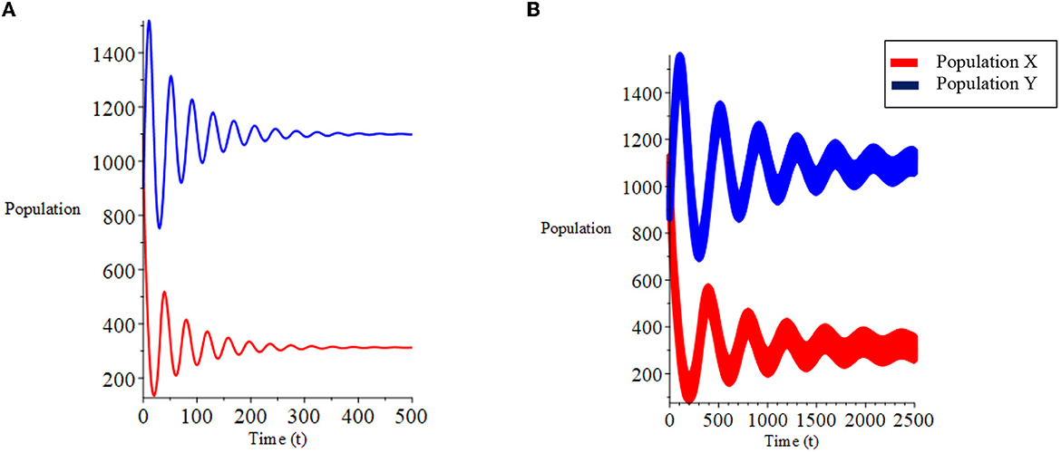
Figure 1. Population growth over time from case (i) of model I. (A) Crisp. (B) Fuzzy.

FIGURE 2

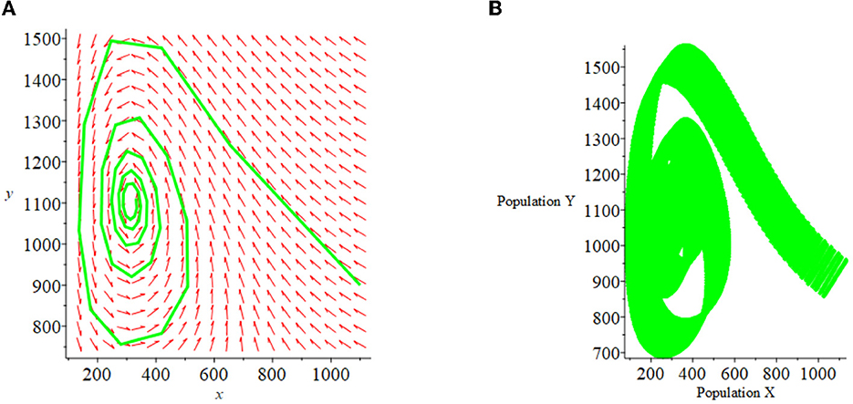
Figure 2. Phase Plane of case (i) of model I. (A) Crisp. (B) Fuzzy.

Let the initial population X₀ and Y₀ uncertain be defined as a triangular fuzzy number with ${\left[X_0\right]}^{\alpha }=\left[1,050+50\alpha ,1,150-50\alpha \right]$ and ${\left[Y_0\right]}^{\alpha }=\left[850+50\alpha ,950-50\alpha \right]$. Based on theorems 3.1 and 3.2, the fuzzy equilibrium points are obtained: χ_{{0, 0}}, χ_{{1, 000, 0}}, and χ_{{312.5, 1099.594}}, where the equilibrium point χ_{{0, 0}} and χ_{{1, 000, 0}} is unstable, and the equilibrium point χ_{{312.5, 1099.594}} is asymptotically stable. The numerical simulation results for the fuzzy model in case (i) are presented in Figures 1, 2B. Figure 1B shows the fuzzy system is stable toward the equilibrium point χ_{{312.5, 1099.594}}. The fuzzy phase plane graph for case (i) is presented in Figure 2B.

Let other than X₀ and Y₀, parameter a is also uncertain and is expressed in triangular fuzzy numbers with [a]^α = [0.4 + 0.1α, 0.6 − 0.1α], then the behavior of the system shown in Figure 3.

FIGURE 3

Figure 3. (A) Population growth over time. (B) Phase plane fuzzy for case (i) of model I with parameter a and population X₀, Y₀ is fuzzy.

The simulation results can be seen that by adding a parameter as a fuzzy number, the dynamic behavior of the fuzzy system qualitatively shows the same results when only the initial populations of prey and predators are fuzzy, and this is in accordance with the behavior of the crisp system.

Case (ii):

For the case (ii) where d < c and $K>\frac{Ac}{d-c}$, three equilibrium points are obtained: (0.0), (1,000, 0), and (−812.5, −1114.973). The point (−812.5, −1114,973) is ignored because it has a negative value, the stability of the equilibrium point is: at point (0,0) is unstable and at point (1,000, 0) is asymptotically stable. The results of the numerical simulation of case (ii) are presented in Figures 4, 5A. Figure 4A shows the system is stable toward the equilibrium point (1,000, 0). The phase plane graph for case (ii) is presented in Figure 5A.

FIGURE 4

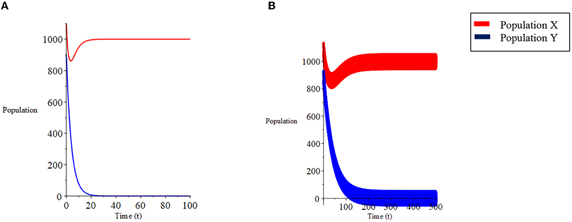
Figure 4. Population growth over time for case (ii) of model I. (A) Crisp. (B) Fuzzy.

FIGURE 5

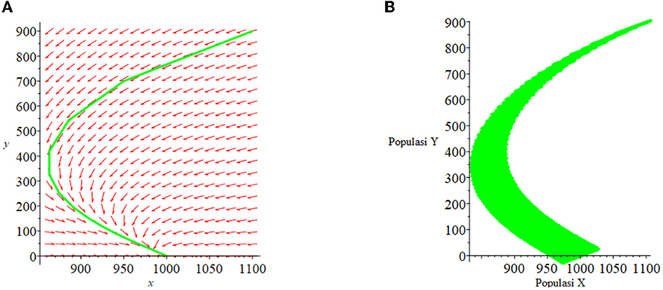
Figure 5. Phase Plane for case (ii) of model I. (A) Crisp. (B) Fuzzy.

Suppose the initial population is uncertain and defined as a triangular fuzzy number as in case (i). Based on theorems 3.1 and 3.2, the fuzzy equilibrium points are obtained: χ_{{0, 0}}, and χ_{{1, 000, 0}}, where at the equilibrium point χ_{{0, 0}} is unstable and at the point χ_{{1, 000, 0}} asymptotically stable. The numerical simulation results for the fuzzy model in case (ii) are presented in Figures 4, 5B. Figure 4B shows the fuzzy system is stable toward the equilibrium point χ_{{1, 000, 0}}. The fuzzy phase plane graph for case (ii) is presented in Figure 5B.

Let other than X₀ and Y₀, parameter a is also uncertain and is expressed in triangular fuzzy numbers as in case (i), then the behavior of the system is shown in Figure 6.

FIGURE 6

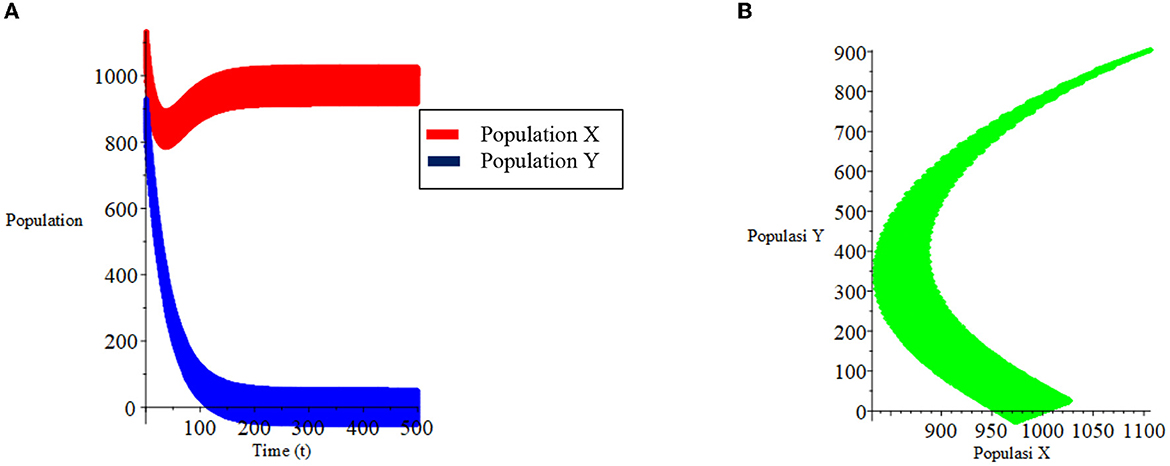
Figure 6. (A) Population growth over time. (B) Phase plane fuzzy for case (ii) of model I with parameter a and population X₀, Y₀ are fuzzy.

The results of the numerical simulation are presented in Figures 1–6 shows that for both cases of model I, the solution graph with the fuzzy approach differs quantitatively, but qualitatively gives the same results as the graph from the crisp system when only the initial population is fuzzy, but slightly different when one of the parameters and the initial population is fuzzy.

Model II: For model II, Numerical simulation is divided into two cases. It is assumed for both cases the values of the parameters and the initial population are the same as for model I: a = 0.5, b = 0.254, K = 1, 000, and A = 500. And other parameters in this model are assumed as follows:

• c = 0.325, d = 0.125, p₁ = 1, p₂ = 2, and E = 0.275

• c = 0.125, d = 0.325, p₁ = 1, p₂ = 1, and E = 0.6

Suppose the initial population of prey and predators is X₀ = 1, 100 and Y₀ = 900.

Case (i):

For case (i) where $E<\frac{a}{p_1}$ obtained three equilibrium points: (0.0), (450,0), and (−583.3, −169.51). The point (−583.3, −169.51) is ignored because it is negative. The stability at equilibrium point (0, 0) is unstable and at (450,0) is asymptotically stable. The numerical simulation results of case (i) are presented in Figures 7, 8A. Figure 7A shows the system is stable toward the point of equilibrium (450.0). The phase plane graph for case (i) is presented in Figure 8A.

FIGURE 7

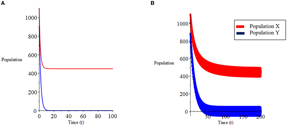
Figure 7. Population growth over time for case (i) of model II. (A) Crisp. (B) Fuzzy.

FIGURE 8

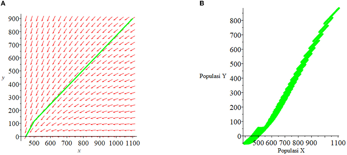
Figure 8. Phase Plane for case (i) of model II. (A) Crisp. (B) Fuzzy.

Suppose the initial population X₀ and Y₀ uncertain is defined as a triangular fuzzy number as in model I, then the fuzzy equilibrium point χ_{{0, 0}} is unstable, and the fuzzy equilibrium point χ_{{450, 0}} is asymptotically stable. The numerical simulation results for the fuzzy model in case (i) are presented in Figures 7, 8B. Figure 7B shows a stable fuzzy system toward the equilibrium point χ_{{450, 0}}. The fuzzy phase plane graph for case (i) is presented in Figure 8B.

Case (ii):

For the case (ii) where $E>\frac{a}{p_1}$ obtained three equilibrium points: (0.0), (−200,0), and (−906.25, −564.792). The points (−200,0) and (−906.25, −564.792) are ignored because they are negative. The numerical simulation results of case (ii) are presented in Figures 9, 10A. Figure 9A shows the system is stable toward the equilibrium point (0,0). The phase plane graph for case (ii) is presented in Figure 10A.

FIGURE 9

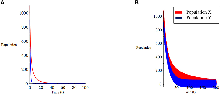
Figure 9. Population growth over time for case (ii) of model II. (A) Crisp. (B) Fuzzy.

FIGURE 10

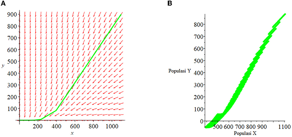
Figure 10. Phase plane for case (ii) of model II. (A) Crisp. (B) Fuzzy.

Suppose the initial population is uncertain and defined as a triangular fuzzy number as in model I, then the fuzzy equilibrium point χ_{{0, 0}} is stable. The numerical simulation results for the fuzzy model in case (ii) are presented in Figures 9, 10B. Figure 9B shows the fuzzy system is stable toward the equilibrium point χ_{{0, 0}}. The fuzzy phase plane graph for case (ii) is presented in Figure 10B.

7. Discussion

The research presented in this paper is an extension of the predator-prey model with a type II Holling functional response discussed by Jha et al. [34] taking into account the uncertainty in the parameters and the initial population expressed in fuzzy numbers. This model is further expanded by adding harvesting factors to both populations. In this study, the behavior of the system is only studied qualitatively by performing numerical simulations to explore the behavior of the fuzzy system and compare it with the crisp system. In conducting the simulation, we use triangular fuzzy numbers to express uncertainty in the initial population and parameters. Of the two models studied, we found the same results. In both models, the fuzzy system shows the same behavior as the crisp system when only the initial population of prey and predators is fuzzy or when one parameter is added as a fuzzy parameter. Another result obtained is, for the fuzzy model, the time required for the system to reach equilibrium is longer than the crisp model. This is due to the uncertainty in the initial value expressed in the fuzzy interval. This research only studied the behavior of the system qualitatively through numerical simulation. In this numerical simulation, all the figures of the phase planes for the fuzzy systems above are plotted for the value of the α-level equals zero. It seems that the phase planes for the crisp systems can be extracted from the fuzzy system's phase planes with the α-level equals zero. This is an interesting result that can be interpreted crisp model can be used as a special case of fuzzy model whenever the degree of uncertainty is relatively low.

8. Conclusion

In this paper, we have developed a numerical scheme to find the solution of two predator-prey models with a Holling type II functional response by considering fuzzy parameters and fuzzy initial populations. The first model was developed from the model studied by Jha et al. [34] by replacing the initial population and one of the parameters with a fuzzy number. While the second model was developed from the first model by adding harvesting factors to both prey and predator populations. The behavior of the model was studied qualitatively using the Runge-Kutta method of order-5 which was modified for the fuzzy system using the Zadeh extension principle. The numerical simulation results show that, when the initial population prey and predators that have fuzzy values, then both fuzzy models have the same behavior as the crisp model, but the fuzzy model takes a longer time to achieve stability than the crisp model. This is due to the uncertainty in the initial population which is indicated by fuzzy intervals. Likewise, when one parameter is added with a fuzzy value, the fuzzy model has the same behavior as the crisp model. Finally, we can conclude that fuzzy behavior represents a generalization of crisp behavior, and this gives more realistic results that represent the problem of uncertainty. However, there are still much work to be done in the future, including studying the stability of the system analytically, bifurcation problems, and others. As pointed by one of the reviewer, it “would have been more interesting to place the choice of parameters on the crisp model exibiting marked sensitivity behavior to initial conditions” and this is currently under investigation by the authors.

Data availability statement

The original contributions presented in the study are included in the article/supplementary material, further inquiries can be directed to the corresponding author.

Author contributions

AS designed and supervised the research. IS developed the scheme and numerical simulations. EC and NA conducted the literature review. All authors contributed to the articles and approved the submitted versions.

Funding

This research was published with funding from Universitas Padjadjaran through the Article Processing Charge (APC) Replacement Scheme.

Conflict of interest

The authors declare that the research was conducted in the absence of any commercial or financial relationships that could be construed as a potential conflict of interest.

Publisher's note

All claims expressed in this article are solely those of the authors and do not necessarily represent those of their affiliated organizations, or those of the publisher, the editors and the reviewers. Any product that may be evaluated in this article, or claim that may be made by its manufacturer, is not guaranteed or endorsed by the publisher.

References

1. Wang Q, Zhai S, Liu Q, Liu Z. Stability and optimal harvesting of a predator-prey system combining prey refuge with fuzzy biological parameters. Math Biosci. Eng. (2021) 18:9094–120. doi: 10.3934/mbe.2021448

PubMed Abstract | CrossRef Full Text | Google Scholar

2. Supriatna AK, Possingham HP. Optimal harvesting for a predator-prey metapopulation. Bull Math Biol. (1998) 60:49–65. doi: 10.1006/bulm.1997.0005

CrossRef Full Text | Google Scholar

3. Supriatna AK, Possingham HP. Harvesting a two-patch predator-prey metapopulation. Nat Resour Model. (1999) 12:481–98. doi: 10.1111/j.1939-7445.1999.tb00023.x

CrossRef Full Text | Google Scholar

4. Dawes JHP, Souza MO. A derivation of Holling's type I, II and III functional responses in predator-prey systems. J Theor Biol. (2013) 327:11–22. doi: 10.1016/j.jtbi.2013.02.017

PubMed Abstract | CrossRef Full Text | Google Scholar

5. Jana S, Kar TK. Modeling and analysis of a prey-predator system with disease in the prey. Chaos Solitons Fract. (2013) 47:42–53. doi: 10.1016/j.chaos.2012.12.002

CrossRef Full Text | Google Scholar

6. Ma Z, Wang S, Wang T, Tang H. Stability analysis of prey-predator system with Holling type functional response and prey refuge. Adv Differ Equat. (2017) 2017:243. doi: 10.1186/s13662-017-1301-4

PubMed Abstract | CrossRef Full Text | Google Scholar

7. Gomes LT, de Barros LC, Bede B. Fuzzy differential equations in various approaches (2015). doi: 10.1007/978-3-319-22575-3

CrossRef Full Text | Google Scholar

8. Mizukoshi MT, Barros LC, Chalco-Cano Y, Román-Flores H, Bassanezi RC. Fuzzy differential equations and the extension principle. Inf Sci. (2007) 177:3627–35. doi: 10.1016/j.ins.2007.02.039

PubMed Abstract | CrossRef Full Text | Google Scholar

9. Bandyopadhyay A, Kar S. System of Type-2 Fuzzy Differential Equations and Its Applications. Vol. 31. London: Springer (2019).

Google Scholar

10. Ahmad MZ, Hasan MK. Modeling of biological populations using fuzzy differential equations. Int J Mod Phys Conf Ser. (2012) 9:354–63. doi: 10.1142/S2010194512005429

CrossRef Full Text | Google Scholar

11. Barros LC, Gomes LT, Tonelli PA. Fuzzy Differential Equations: An Approach via Fuzzification of the Derivative Operator. Vol. 230. Elsevier (2013). doi: 10.1016/j.fss.2013.03.004

CrossRef Full Text | Google Scholar

12. Alamin A, Mondal SP, Alam S, Goswami A. Solution and stability analysis of non-homogeneous difference equation followed by real life application in fuzzy environment. Sadhana Acad Proc Eng Sci. (2020) 45:185. doi: 10.1007/s12046-020-01422-1

CrossRef Full Text | Google Scholar

13. Mizukoshi MT, Barros LC, Bassanezi RC. Stability of fuzzy dynamic systems. Int Uncertain J Fuzziness Knowl Based Syst. (2009) 17:69–83. doi: 10.1142/S0218488509005747

CrossRef Full Text | Google Scholar

14. Jayakumar T, Maheskumar D, Kanagarajan K. Numerical solution of fuzzy differential equations by Runge Kutta method of order five. Appl Math Sci. (2012) 6:2989–3002. doi: 10.17654/FS021020135

CrossRef Full Text | Google Scholar

15. Nayak S, Chakraverty S. Numerical solution of fuzzy stochastic differential equation. J Intell Fuzzy Syst. (2016) 31:555–63. doi: 10.3233/IFS-162168

PubMed Abstract | CrossRef Full Text | Google Scholar

16. Behroozpoor AA, Vahidian Kamyad A, Mazarei MM. Numerical solution of fuzzy initial value problem (FIVP) using optimization. Int J Adv Appl Sci. (2016) 3:36–42. doi: 10.21833/ijaas.2016.08.007

CrossRef Full Text | Google Scholar

17. Tapaswini S, Chakraverty S. Numerical solution of Fuzzy arbitrary order predator-prey equations. Appl Appl Math Int J. (2013) 8:647–72.

Google Scholar

18. Tapaswini S, Chakraverty S. A New approach to fuzzy initial value problem by improved euler method. Fuzzy Inf Eng. (2012) 4:293–312. doi: 10.1007/s12543-012-0117-x

CrossRef Full Text | Google Scholar

19. da Silva Peixoto M, de Barros LC, Bassanezi RC. Predator-prey fuzzy model. Ecol Model. (2008) 214:39–44. doi: 10.1016/j.ecolmodel.2008.01.009

CrossRef Full Text | Google Scholar

20. Pandit P, Singh P. Prey Predator Model With Fuzzy Initial Conditions. International Journal of Web Engineering and Technology (IJEIT). Vol. 3. (2014). p. 65–8.

PubMed Abstract | Google Scholar

21. Ak O, Oru O. A Prey Predator Model With Fuzzy Initial Values. Hacettepe Journal of Mathematics and Statistics. Vol. 41. (2012). p. 387–95.

Google Scholar

22. Ahmad MZ, De Baets B. A predator-prey model with fuzzy initial populations. In: 2009 International Fuzzy Systems Association world congress and 2009 European Society of Fuzzy Logic and Technology. (2009). p. 1311–4. Available online at: https://www.researchgate.net/publication/221399560_A_Predator-Prey_Model_with_Fuzzy_Initial_Populations

Google Scholar

23. Narayanamoorthy S, Baleanu D, Thangapandi K, Perera SSN. Analysis for fractional-order predator–prey model with uncertainty. IET Syst Biol. (2019) 13:277–89. doi: 10.1049/iet-syb.2019.0055

PubMed Abstract | CrossRef Full Text | Google Scholar

24. Omar AHA, Ahmed IAA, Hasan YA. The fuzzy ratio prey-predator model. Int J Comput Sci Electron Eng. (2015) 3:101–6.

Google Scholar

25. Pal D, Mahapatra GS, Samanta GP. Parameter uncertainty in biomathematical model described by one-prey two-predator system with mutualism. Int J Biomath. (2017) 10:1750082. doi: 10.1142/S1793524517500826

CrossRef Full Text | Google Scholar

26. Mallak S, Farekh D, Attili B. Numerical investigation of fuzzy predator-prey model with a functional response of the form arctan(ax). Mathematics. (2021) 9:17–9. doi: 10.3390/math9161919

CrossRef Full Text | Google Scholar

27. Pal D, Mahapatra GS, Samanta GP. Stability and bionomic analysis of fuzzy prey–predator harvesting model in presence of toxicity: a dynamic approach. Bull Math Biol. (2016) 78:1493–519. doi: 10.1007/s11538-016-0192-y

PubMed Abstract | CrossRef Full Text | Google Scholar

28. Yu X, Yuan S, Zhang T. About the optimal harvesting of a fuzzy predator–prey system: a bioeconomic model incorporating prey refuge and predator mutual interference. Nonlinear Dyn. (2018) 94:2143–60. doi: 10.1007/s11071-018-4480-y

CrossRef Full Text | Google Scholar

29. Pal D, Mahapatra GS, Samanta GP. Stability and bionomic analysis of fuzzy parameter based prey–predator harvesting model using UFM. Nonlinear Dyn. (2015) 79:1939–55. doi: 10.1007/s11071-014-1784-4

CrossRef Full Text | Google Scholar

30. Meng XY, Wu YQ. Dynamical analysis of a fuzzy phytoplankton–zooplankton model with refuge, fishery protection and harvesting. J Appl Math Comput. (2020) 63:361–89. doi: 10.1007/s12190-020-01321-y

CrossRef Full Text | Google Scholar

31. Mahata A, Mondal SP, Roy B, Alam S. Study of two species prey-predator model in imprecise environment with MSY policy under different harvesting scenario. Environ Dev Sustain. (2021) 23:14908–32. doi: 10.1007/s10668-021-01279-2

CrossRef Full Text | Google Scholar

32. Pal D, Mahapatra GS, Samanta GP. A study of bifurcation of prey-predator model with time delay and harvesting using fuzzy parameters. J Biol Syst. (2018) 26:339–72. doi: 10.1142/S021833901850016X

CrossRef Full Text | Google Scholar

33. de Barros LC, Bassanezi RC, Lodwick WA. Studies in Fuzziness and Soft Computing A First Course in Fuzzy Logic, Fuzzy Dynamical Systems, and Biomathematics Theory and Applications Berlin: Springer (2017).

34. Jha P, Ghorai S. Stability of prey-predator model with Holling type response function and selective harvesting. J Appl Comput Math. (2017) 6:3. doi: 10.4172/2168-9679.1000358

CrossRef Full Text | Google Scholar

35. Das T, Mukherjee RN, Chaudhuri KS. Bioeconomic harvesting of a prey–predator fishery. J Biol Dyn. (2009) 3:447–62. doi: 10.1080/17513750802560346

PubMed Abstract | CrossRef Full Text | Google Scholar