Mathematical analysis of the impact of community ignorance on the population dynamics of dengue

This study proposes a dengue spread model that considers the nonlinear transmission rate to address the level of human ignorance of dengue in their environment. The SIR − UV model has been proposed, where SIR denotes the classification of the human population and UV denotes the classification of the mosquito population. Assuming that the total human population is constant, and the mosquito population is already in its steady-state condition, using the Quasi-Steady State Approximation (QSSA) method, we reduce our SIR − UV model into a more simple IR-model. Our analytical result shows that a stable disease-free equilibrium exists when the basic reproduction number is <1. Furthermore, our model also shows the possibility of a backward bifurcation. The more ignorant the society is about dengue, the higher the possibility that backward bifurcation phenomena may appear. As a result, the condition of the basic reproduction number being <1 is insufficient to guarantee the extinction of dengue in a population. Furthermore, we found that increasing the recovery rate, reducing the waning immunity rate, and mosquito life expectancy can reduce the possibility of backward bifurcation phenomena. We use dengue incidence data from Jakarta to calibrate the parameters in our model. Through the fast Fourier transform analysis, it was found that dengue incidence in Jakarta has a periodicity of 52.4, 73.4, and 146.8 weeks. This result indicates that dengue will periodically appear at least every year in Jakarta. Parameter estimation for our model parameters was carried out by assuming the infection rate of humans as a sinusoidal function by determining the three most dominant frequencies. Numerical and sensitivity analyses were conducted to observe the impact of community ignorance on dengue endemicity. From the sensitivity analysis, we found that, although a larger community ignorance can trigger a backward bifurcation, this threshold can be minimized by increasing the recovery rate, prolonging the temporal immunity, or reducing the mosquito population. Therefore, to control dengue transmission more effectively, media campaigns undertaken by the government to reduce community ignorance should be accompanied by other interventions, such as a good treatment in the hospital or vector control programs. With this combination of interventions, it will be easier to achieve a condition of dengue-free population when the basic reproduction number is less than one.

1. Introduction

Dengue is an infectious disease that is caused by the dengue virus (DEN virus or DENV). This virus is transmitted through the bite of an infected female Aedes aegypti or Aedes albopictus [1, 2]. It is estimated that ~50% of the world population is at risk of dengue every year [3]. Dengue has been the subject of main concern in many tropical and subtropical countries, including Indonesia. Since the first case of dengue in Indonesia was reported in Jakarta and Surabaya way back in 1968, the incidence of dengue in Indonesia continues to spread to this day [4]. Based on a new report from the Ministry of Health Indonesia, from early 2022 until 20 February 2022, the cumulative number of dengue cases was recorded as 13,776 cases. Meanwhile, the number of deaths due to dengue was recorded as 145 cases [5].

There are four different serotypes of DENV, namely, DENV-1, DENV-2, DENV-3, and DENV-4 [6, 7]. In many cases, the primary infection of dengue is often asymptomatic. In contrast, the secondary infection with different serotypes from the primary infection may develop more severe symptoms, such as bone pain and headache, up to more occasionally fatal symptoms [8, 9]. Individuals who have already recovered from the primary infection will maintain a lifelong immunity to the first DENV that had caused the primary infection, but only temporal to the other three serotypes [10]. When the short-term immunity to other serotypes wanes, the recovered individuals may acquire a secondary infection that can be even more severe than the primary infection. This phenomenon is called the ADE process [11, 12].

There is no specific treatment to cure dengue-infected individuals of the disease. The main action plan to treat dengue-infected individuals is rendered feasible by giving them supportive care, or if the case is severe, then the patient requires hospitalization which becomes an obligation to be done. Recently, several candidates for dengue vaccines have been in the process of development [13, 14]. An affordable and effective dengue vaccine will give importance to the control of dengue spread around the world. The main control program adopted by many governments worldwide to control the spread of dengue is the vector control program and steps are taken to reduce the probability of a successful infection through a mosquito repellent. Another option to prevent the spread of dengue (and other diseases) is by developing community awareness on the danger of the disease [15–18]. Community participation in eliminating or at least suppressing the spread of dengue can be done through several activities, such as through media campaigns to disseminate knowledge about how to prevent acquiring infection from mosquitoes from individual levels up to community levels. The author in [15] implies that the risk of dengue may be increased when there is a lack of community awareness due to misunderstanding between the community and the government. Therefore, maintaining community awareness by reducing the ignorance of dengue is essential to guarantee intervention success in controlling the spread of dengue.

Mathematical models have been used widely by researchers to understand how vector-borne diseases spread among the population [19–23]. For the dengue transmission model, many authors have used mathematical modeling to guide public health strategies to control the spread of dengue. The mathematical modeling process is very challenging due to the complexity of the dengue transmission mechanism. A more complex model may bring in a more realistic modeling, but finding the analytical results and conclusion often entails difficulty. Hence, the researcher needs to develop a realistic but simple model with realistic assumptions. The use of real incidence data is also needed to calibrate the performance of the model. There are many approaches that can be used to construct the dengue transmission model, such as with ordinary differential equations [24, 25], partial differential equations [26, 27], fractional-order differential equations [28, 29], stochastic differential equations [30–32], and other approaches.

Many mathematical models for dengue transmission use a deterministic approach. Although the transmission process of dengue involves a vector animal (Aedes mosquito) as the prime spreader, some authors use a host-to-host modeling approach [30, 33, 34]. This approach does not involve the dynamics of mosquitoes in their model since it can be argued that the mosquitoes' life expectancy is very short compared to the human life expectancy. Hence, the dynamic of mosquitoes is much faster compared to that of the human. The authors in [35] find that the only essential dynamics are coming from the human population, and mosquito dynamics only slightly perturb them. The other approach is adopted by considering the dynamic of mosquitoes [24, 25]. With this approach, the mosquito population is explicitly involved in the model. With the involvement of mosquito dynamics, such implementation of vector control can be modeled into the equation. When the vector control is involved in the model, an optimal control approach can be used to understand the short-term impact of the intervention and determine the most effective strategy [36–38]. Modeling dengue transmission is not only for the macro scale (population scale). Some of the authors also construct the model to understand the dynamic within the host [39, 40]. This modeling is conducted to understand the interaction between the free virus with susceptible targeted cells. Some interesting factors are involved in this modeling approach, such as the infectivity of the virus and immune response.

From the aspect of the impact of community awareness on the dengue transmission model, there are some models which have been introduced by authors. The authors in [41] introduced a mathematical model of dengue where the effect of media awareness was included. Mathematical analysis on the equilibrium points and the basic reproduction number was included in it. The author in [42] introduced a multistrain dengue model that combined mosquito control programs and human awareness. They found that the control of a large number of mosquitoes and human awareness was required to control dengue effectively. The author introduced an optimal control problem of dengue with human awareness and vector control in [43]. The authors used Pontryagin's maximum principle to characterize the necessary conditions for the optimal control problem. The author in [44] introduced a modified host–vector model by considering low- and high-risk susceptible populations. The author analyzed global stability on all equilibrium points. The author in [45] introduced an optimal control model of dengue transmission. The author developed the model by considering five control variables: information spread, bed nets, treatment, screening, and insecticide. The impact of a media campaign that can reduce the rate of infection was developed by the author in [24]. The author conducted a cost-effectiveness analysis to understand the most cost-effective strategy that can be employed to control dengue transmission. Recently, the authors in [25] combined vaccination, vector control, and media campaign in their model where the seasonality was accommodated. All the mentioned references consider the same assumption that (1) aware individuals have a smaller probability of being infected due to their awareness and (2) more prominent infected individuals will reduce the infection rate more. The second assumption is reasonable when we wish to model the spread of dengue among a population where awareness of dengue could increase the participation of the population in the dengue control programs.

To calibrate the proposed dengue model, many authors use incidence data to estimate their parameters. The idea behind this development is to find the best-fit parameters, such that the model simulation output can fit the time series of the data. Please see the following references for the use of incidence data in their dengue research: Aguiar and Stollenwerk [30], ten Bosch et al. [31], Aguiar et al. [34], and Aldila et al. [46]. With this parameter estimation, the researcher can make a short time prediction on their model. Some interventions can be included in their model and the possible outcomes predicted in the near future.

Motivated by the above discussion, no authors had discussed the impact of community ignorance on the spread of dengue. In this circumstance, more infected individuals will increase the probability of infection in the human and mosquito populations. In some countries where dengue fever continues to emerge throughout the year, the level of public ignorance of the spread of dengue fever is no longer as high as for several newly discovered diseases and it is quite a concern, such as Zika in 2018 or COVID-19 in the late 2019. Hence, it is important to consider the community's ignorance of our proposed model. Based on this background, here in this article, we introduce our SIR-UV mathematical model to describe the spread of dengue under the impact of community ignorance. The Quasi-Steady State Approximation method was used to simplify the model. We used the weekly incidence data of dengue from Jakarta during the period from January 2008 to December 2021 to estimate the parameter values in our model. We used the fast Fourier transform to extract the most significant frequency from our data. With this dominant frequency, we fit our model output with the data by assuming the infection rate as a sinusoidal function that depends on time. Some mathematical and numerical analyses were conducted to understand the qualitative behavior of our model and how it was related to the basic reproduction number. Furthermore, we also analyzed how community ignorance can trigger the appearance of a backward bifurcation, which can cause dengue to exist, even though the basic reproduction number is already <1. The layout of this article is as follows: In Section 2, we construct our model. In the same section, we perform our data assimilation to find out the best-fit parameters of our model. The model analysis is given in Section 3, which is followed by some sensitivity analyses and numerical experiments in Section 4. The concluding remarks are given in Section 5.

2. Mathematical model and data assimilation

2.1. Model formulation

To develop our dengue transmission model, we introduce N and M as the total human and female Aedes sp. populations. Let the total human population be classified into Susceptible, Infected, and Recovered compartments, which are denoted by S, I, and R, respectively. On the other hand, the mosquito population is only classified into Susceptible and Infected compartments, which are denoted by U and V, respectively. Due to the short life expectancy of mosquitoes, we do not consider the recovery process in the mosquito population. Since dengue does not transmit vertically to newborns, we assume that the recruitment rates of a human and mosquitoes are going to be susceptible. The rates of a newborn human and mosquitoes are given by Λ_h and Λ_v, respectively. Susceptible humans can get infected by dengue only if infected mosquitoes bite them. In many countries where dengue become can be found all-year round, for instance in Indonesia, public awareness of dengue fever is not as high as that of new disease incidents such as COVID-19. Cases of dengue fever only received attention when the cases were already very high and made the hospital unable to accommodate the increasing number of patients. Due to these phenomena, the authors feel that it is important to discuss the factors of public neglect of news on dengue fever. Based on this assumption, we notice that the infection rate will increase when the number of infected individuals increases. Therefore, the incidence of infection will occur at a much faster pace compared to the standard mass action infection function (β_hSV), where β_h is the infection rate in the human population. Hence, we assume that the infection rate is nonlinear and depends on the number of infected individuals. In this case, we choose β_h(I) = β_h(1 + αI), where α > 0 represents the incidence increasing factor due to community ignorance against dengue. For a further discussion on this type of function, please see [47]. Based on this assumption, we have β_h(1 + αI)SV as the total number of new infections of susceptible individuals due to contact with infected mosquitoes with a probability of infection β_h. Based on similar arguments, we derived that the rate of new infected mosquitoes is given by β_v(1 + αI)UI, where β_v is the infection rate of dengue in the mosquito population. Let γ be the recovery rate, δ the waning rate of temporal immunity, μ_h the natural death rate of a human, and μ_v the natural death rate of mosquitoes, we have the dynamic of dengue transmission under a nonlinear infection rate as given in system (1).

$\begin{array}{ll}\begin{array}{c}\frac{dS}{dt}={\Lambda }_h-{\beta }_h(1+\alpha I)SV+\delta R-{\mu }_{h}S,\hfill \\ \frac{dI}{dt}={\beta }_h(1+\alpha I)SV-\gamma I-{\mu }_{h}I,\hfill \\ \frac{dR}{dt}=\gamma I-\delta R-{\mu }_{h}R.\hfill \\ \frac{dU}{dt}={\Lambda }_v-{\beta }_v(1+\alpha I)UI-{\mu }_{v}U,\hfill \\ \frac{dV}{dt}={\beta }_v(1+\alpha I)UI-{\mu }_{v}V,\hfill \end{array}\hfill & (1)\end{array}$

with an initial condition S(0) > 0, I(0) ≥ 0, R(0) ≥ 0, U(0) > 0, V(0) ≥ 0. Our model is well defined both mathematically and biologically. Please see Theorem 1 for the non-negative solution property of each variable of system (1) and the feasible region of the solution in Theorem 2.

THEOREM 1. Model (1) with initial condition S(0) > 0, I(0) ≥ 0, R(0) ≥ 0, U(0) > 0, V(0) ≥ 0 always has a non-negative solution for all times t ≥ 0.

PROOF. We use an integrating factor to solve this theorem. Under the given initial conditions, from $\frac{dS}{dt}$ in system (1), we have

$\begin{array}{l}\frac{dS}{dt}={\Lambda }_h-{\beta }_h(1+\alpha I)SV+\delta R-{\mu }_{h}S.\end{array}$

It can be written as

$\begin{array}{ll}\frac{dS}{dt}+A(t)S=B(t)& (2)\end{array}$

where

$\begin{array}{l}A(t)={\beta }_h(1+\alpha I)V+{\mu }_h,\\ B(t)={\Lambda }_h+\delta R,\end{array}$

Define an integrating factor $C(t)=e^{{\int }_0^{T}A(t)dt}$ and multiply (2) with the integrating factor. Hence, we have

$\begin{array}{l}{e}^{{\int }_0^{T}A(t)dt}\frac{dS}{dt}+e^{{\int }_0^{T}A(t)dt}A(t)S=e^{{\int }_0^{T}A(t)dt}B(t).\end{array}$

It can be written as

$\begin{array}{l}{D}_t[S(t)e^{{\int }_0^{T}A(t)dt}]=e^{{\int }_0^{T}A(t)dt}B(t).\end{array}$

By integrating both sides of the above equation, we obtain

$\begin{array}{l}{\displaystyle {\int }_0^T}{D}_t[S(t)e^{{\int }_0^{T}A(t)dt}]dt={\displaystyle {\int }_0^T}{e}^{{\int }_0^{T}A(t)dt}B(t)dt.\end{array}$

Therefore,

$\begin{array}{l}S(T)=e^{-{\int }_0^{T}A(t)dt}({\displaystyle {\int }_0^T}{e}^{{\int }_0^{T}A(t)dt}B(t)dt+S_0)>0.\end{array}$

In a similar way, it can be shown that I(t) ≥ 0, R(t) ≥ 0, U(t) > 0, and V(0) ≥ 0, under the given initial condition I₀ ≥ 0, R₀ ≥ 0, U₀ > 0, and V₀ ≥ 0. Thus, the solutions of S(t), I(t), R(t), U(t), and V(t) are non-negative for all times t > 0.t

THEOREM 2. Model (1) with initial condition S(0) > 0, I(0) ≥ 0, R(0) ≥ 0, U(0) > 0, V(0) ≥ 0 is bounded in the region

$\begin{array}{ll}\begin{array}{c}\Omega =\{(S,I,R,U,V)\in {ℝ}_5^{+}\cup 0_5:N=S+I+R\\ =\frac{{\Lambda }_h}{{\mu }_h},M=U+V=\frac{{\Lambda }_v}{{\mu }_v}\}.\end{array}& (3)\end{array}$

PROOF. From model (1), we obtain

$\begin{array}{l}\begin{array}{c}\frac{dN}{dt}={\Lambda }_h-{\mu }_{h}N.\\ \frac{dM}{dt}={\Lambda }_v-{\mu }_v.\hfill \end{array}\hfill \end{array}$

We assume that the total population of human and mosquito is constant, so we obtain the system bounded in $N=\frac{{\Lambda }_h}{{\mu }_h}$ and $M=\frac{{\Lambda }_v}{{\mu }_v}$. Hence, all feasible solutions of model (1) enter the region

$\begin{array}{l}\Omega =\{(S,I,R,U,V)\in {ℝ}_5^{+}\cup 0_5:N=S+I+R=\frac{{\Lambda }_h}{{\mu }_h},\\ M=U+V=\frac{{\Lambda }_v}{{\mu }_v}\}.\end{array}$

2.2. A quasi-steady state approximation

It is approximated that the life expectation of a mosquito is 30 days [48]. Considering human life expectation, which is around 70 years [49], a mosquito population can reach its equilibrium in a much shorter duration compared to a human population. It indicates that the mosquito population has a fast dynamics, while the human population has a slow dynamics. Based on this assumption, we may assume that the mosquito populations have already reached their equilibrium condition in our simulation time interval. Hence, using the quasi-steady state approximation, taking $\frac{dU}{dt}=0$ and $\frac{dV}{dt}=0$, gives us

$\begin{array}{l}\begin{array}{c}{U}^{*}=\frac{{\Lambda }_v}{{\beta }_v(1+\alpha I)I+{\mu }_v},\hfill \\ V^{*}=\frac{{\beta }_v(1+\alpha I){\Lambda }_v}{({\beta }_v(1+\alpha I)I+{\mu }_v){\mu }_v}.\end{array}\hfill \end{array}$

Substituting the above quasi-steady state approximation of (U^*, V^*) in model (1), we have

$\begin{array}{ll}\begin{array}{c}\frac{dS}{dt}={\Lambda }_h-{\beta }_h(1+\alpha I)+\delta R-{\mu }_{h}S,\hfill \\ \frac{dI}{dt}=\frac{{\beta }_h{(1+\alpha I)}^{2}SI{\beta }_v{\Lambda }_v}{((1+\alpha I)I{\beta }_v+{\mu }_v){\mu }_v}-(\gamma +{\mu }_h)I,\hfill \\ \frac{dR}{dt}=\gamma I-\delta R-{\mu }_{h}R.\hfill \end{array}& (4)\end{array}$

Assuming that the total human population is constant. Then, we have S = N − I − R. Hence, the system (4) now reads as

$\begin{array}{ll}\begin{array}{c}\frac{dI}{dt}=\frac{{\beta }_h{(1+\alpha I)}^2(N-I-R)IM}{((1+\alpha I)I+{\kappa }_v)}-(\gamma +{\mu }_h)I,\hfill \\ \frac{dR}{dt}=\gamma I-\delta R-{\mu }_{h}R.\hfill \end{array}\hfill & (5)\end{array}$

where ${\kappa }_v=\frac{{\mu }_v}{{\beta }_v}$ and $M=\frac{{\Lambda }_v}{{\mu }_v}$. The simple IR-model in system (5) has an advantage compared to the original SIRUV-model in system (1) from the perspective of data assimilation, which will be described in the next section. Furthermore, we will analyze the IR-model in system (5) to understand the long time behavior of the SIRUV-model.

2.3. Data assimilation

Jakarta is the capital of Indonesia with a total population of more than 10 million people based on the census data of 2022. The temperature in Jakarta is relatively stable throughout the year, between 24 and 33°C. The highest temperatures are recorded between August and early November. The rainy season in Jakarta falls between October and May every year with more than a 47% chance of a rainy day. The highest rainfall occurs in January with the average rainfall of 22.6 days [50].

Dengue fever has become an annual problem in Indonesia, including Jakarta. The number of dengue fever cases in Jakarta during 2008 to December 2021 can be seen in Figure 1A. High cases of dengue fever are always associated with a high rainfall in Jakarta. The existing literature indicates that the high cases of dengue fever follow a seasonal (periodic) pattern. Based on this observation, it is necessary to analyze the existence of periodicity in the data of dengue fever cases in Jakarta city. Therefore, we apply a fast Fourier transform to our data, and the result can be seen in Figure 1B. From Figure 1B, we show that the three dominant frequencies are 0.019, 0.013, and 0.006. These frequencies are correlated to a periodicity of 52.43, 73.4, and 146.8 weeks, respectively.

FIGURE 1

Figure 1. (A) The number of weekly infected dengue individuals in Jakarta from January 2008 to December 2021. (B) The result of fast Fourier transform analysis from dengue data in Jakarta.

Our aim in this section is to calibrate our proposed mathematical models with the real situation in the field. To do this, we construct a model fitting that involves parameter estimation, which includes the identification of the parameter values that can fit between the model solution [variable I in system (5)] with the incidence data in Figure 1A. For the purpose of parameter estimation, we used the “fmincon” toolbox in Matlab. Fmincon can be used to find the minimum of constrained nonlinear multivariable functions.

As we mentioned earlier, our incidence data indicate a periodic solution. To capture this phenomenon, we treat the infection rate β_h as a sinusoidal parameter, which is given by

$\begin{array}{ll}{\beta }_h(t)=a+{\displaystyle \sum _{i=1}^3}{b}_{i}cos(2\pi d_{i}t)+c_{i}sin(2\pi d_{i}t),\hfill & (6)\end{array}$

where a is the median value of β_h(t), b_i, and c_i are the amplitudes of β_h(t), while d_i refers to the frequencies of β_h(t). Our problem lies in minimizing the Euclidean distance between our model solution [I(t)] and the time series data in Figure 1A using the best-fit parameter β_h(t) with model in (5) as the constraint. This task reads as minimizing the following cost function

$\begin{array}{ll}\mathcal{J}=\frac{1}{2\omega }{\displaystyle \sum _{t=1}^{734}}{(I^{\text{solution}}-I^{\text{data}})}^2,& (7)\end{array}$

where ω is the variance of the data and I^solution is the solution of I(t) from

$\begin{array}{ll}\begin{array}{c}\frac{dI}{dt}=\frac{\left(a+{\displaystyle {\sum }_{i=1}^3}{b}_{i}cos(2\pi d_{i}t)+c_{i}sin(2\pi d_{i}t)\right){(1+\alpha I)}^2(N-I-R)IM}{((1+\alpha I)I+{\kappa }_v)}\hfill \\ -(\gamma +{\mu }_h)I,\hfill \\ \frac{dR}{dt}=\gamma I-\delta R-{\mu }_{h}R.\hfill \end{array}\hfill & (8)\end{array}$

Our task is to find the best-fit parameter Γ₁ = {a, b_i, c_i, d_i, α, κ_v} and the best initial condition Γ₂ = {I(t = 0), R(t = 0)}. We choose other parameter values as follows:

$N=\mathrm{10 000 000},M=2N(\text{assumption}),\gamma =\frac{1}{4},$

[51], [52]

$\begin{array}{c}{\mu }_h=\frac{1}{70\times 52},\delta =\frac{1}{9\times 4}.\hfill \end{array}$

[49], [51]

The result of the parameter estimation is given in Figure 2, while the parameter values and the initial condition are given in Table 1. We can see that our model can fit the qualitative behavior of the data such as the time when the outbreak appears and also when it decreases. However, our model cannot fit the data in all simulation times. We extend our simulation time for the next 2 years until December 2023. We can see that the peak of dengue cases in Jakarta is expected to still appear around April 2022 and March 2023.

TABLE 1

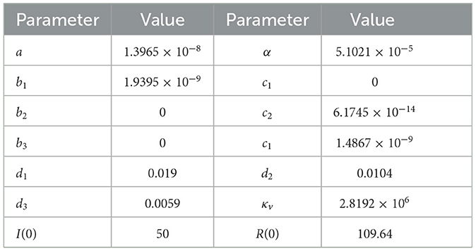
Table 1. Best-fit parameter of system (8) for Figure 2.

FIGURE 2

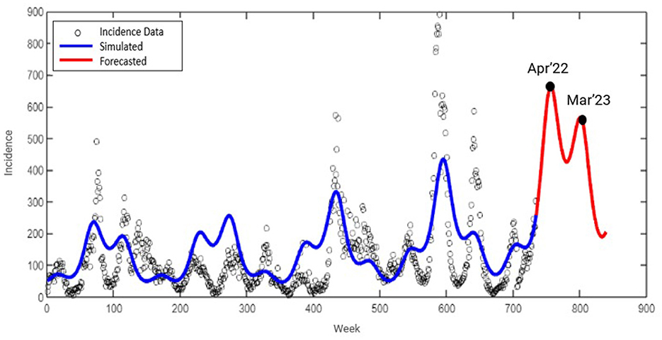
Figure 2. Fitted dengue cases I(t), for the model (8), using data from Jakarta from 2008 to 2021.

3. Model analysis

3.1. Equilibrium points and the basic reproduction number

The dengue-free equilibrium of system (5) is given by

$\begin{array}{ll}(I,R)=(0,0).& (9)\end{array}$

In this case, since S = N − I − R, then the complete model gives the dengue-free equilibrium as given by (S, I, R) = (N, 0, 0). Next, we calculate the respected basic reproduction number of system (5). The basic reproduction number $({\mathcal{R}}_0)$ in the context of dengue is the expected number of secondary cases (in human/mosquitoes) due to one bite of infected/susceptible mosquito to susceptible/infected human, respectively, during its infection period in a fully susceptible population. To calculate the respected basic reproduction number of system (5), we use the next-generation matrix approach introduced by the authors in [53]. First, we calculate the Jacobian matrix of the infected subcompartment of system (5) evaluated in the dengue-free equilibrium in (9). This matrix is given by:

$\begin{array}{l}\mathcal{J}=\left[\frac{{\beta }_{h}NM}{{\kappa }_v}-\gamma -{\mu }_h\right].\end{array}$

Next, we can decompose $\mathcal{J}$ as $\mathcal{F}+\mathcal{V}$, where $\mathcal{F}$ is the transmission matrix and $\mathcal{V}$ is the transition matrix. Hence, we have $\mathcal{F}=\left[\frac{{\beta }_{h}NM}{{\kappa }_v}\right]$ and $\mathcal{V}=[-\gamma -{\mu }_h$. Therefore, the next-generation matrix of system (5) is given by:

$\begin{array}{l}\mathcal{K}={\mathcal{FV}}^{-1}=\left[\frac{{\beta }_{h}NM}{{\kappa }_v(\gamma +{\mu }_h)}\right].\end{array}$

Therefore, the basic reproduction number of system (5), which is taken by the spectral radius of $\mathcal{K}$, is given by:

$\begin{array}{ll}{\mathcal{R}}_0=\frac{{\beta }_{h}NM}{{\kappa }_v(\gamma +{\mu }_h)}.& (10)\end{array}$

In many epidemiological models [], many authors can find the relation between the disease extinction with a condition of ${\mathcal{R}}_0>1$. In our proposed dengue model, we find this relation in the following theorem.

THEOREM 3. The dengue-free equilibrium of system (5) is locally asymptotically stable if ${\mathcal{R}}_0<1$, and unstable if ${\mathcal{R}}_0>1$.

PROOF. We use standard linearization to prove the theorem. Linearization around the dengue-free equilibrium is given by

$\begin{array}{l}\text{J}{|}_{DFE}=\left[\begin{array}{cc}\frac{{\beta }_{h}NM}{{\kappa }_v}-\gamma -{\mu }_h& 0\\ \gamma & -\delta -{\mu }_h\end{array}\right].\end{array}$

Eigenvalues of the above linearization matrix are given by

$\begin{array}{l}{\lambda }_1=\frac{{\beta }_{h}NM}{{\kappa }_v}-\gamma -{\mu }_h,{\lambda }_2=-\delta -{\mu }_h.\end{array}$

Equilibrium is asymptotically stable if all the real parts of its eigenvalues are negative. All of our parameters are positive, therefore the second eigenvalue has negative real parts. To prove that the first eigenvalue has a negative real part, it must be assumed that $\frac{{\beta }_{h}NM}{{\kappa }_v(\gamma +{\mu }_h)}<1\iff {\mathcal{R}}_0<1$.     □

The second equilibrium point is the endemic equilibrium point, which is given by:

$\begin{array}{ll}(I,R)=\left(I^{*},\frac{\gamma I}{\delta +{\mu }_h}\right).& (11)\end{array}$

where I^* is taken from the positive roots of the following third-degree polynomial

$\begin{array}{ll}F(I,\tau )=a_3{I}^3+a_2{I}^2+a_{1}I+a_0=0,& (12)\end{array}$

where τ = {β_h, M, N, α, γ, δ, κ_v, μ_h}, and

$\begin{array}{l}\begin{array}{c}{a}_3={\beta }_{h}M{\alpha }^2(\gamma +{\mu }_h+\delta ),\hfill \\ a_2=M{\beta }_h(N\alpha (\delta +{\mu }_h)-2(\delta +\gamma +{\mu }_h))-(\delta +{\mu }_h)(\gamma +{\mu }_h),\hfill \\ a_1=(M{\beta }_h+{\mu }_h)(\delta +\gamma +{\mu }_h)+\delta \gamma -MN\alpha {\beta }_h(\delta +{\mu }_h),\hfill \\ a_0=-(\delta +{\mu }_h)(\gamma +{\mu }_h){\kappa }_v({\mathcal{R}}_0-1).\hfill \end{array}\hfill \end{array}$

Since $a_0<0\iff {\mathcal{R}}_0>1$ and a₃ > 0, then we have the following theorem.

THEOREM 4. The dengue IR-model in system (5) always has at least one dengue-endemic equilibrium point if ${\mathcal{R}}_0>1$.

PROOF. Since a₃ > 0, then $\underset{I\to -\infty }{lim}F(I,\tau )=-\infty$ and $\underset{I\to \infty }{lim}F(I,\tau )=\infty$. For special cases when ${\mathcal{R}}_0=1$, we have one zero root of F(I, τ). Hence, when a₀ < 0 which is equivalent to ${\mathcal{R}}_0>1$, then the graphic of F(I, τ) will be shifted downward as far as a₀ is concerned. Hence, we have at least one new positive root I of F(I, τ) when ${\mathcal{R}}_0>1$.     □

Since the sign of a₁ is not always positive or negative, it is possible to have another dengue endemic equilibrium when ${\mathcal{R}}_0<1$. Furthermore, since the existence of the dengue-endemic equilibrium point depends on a third-degree polynomial, it is possible to have more than one dengue-endemic equilibrium point.

THEOREM 5. There exists a dengue-endemic equilibrium when ${\mathcal{R}}_0<1$ if α > α^*, where ${\alpha }^{*}=\frac{(\gamma +{\mu }_h+\delta ){\kappa }_v+N(\delta +{\mu }_h)}{2(\delta +{\mu }_h)N{\kappa }_v}$.

PROOF. Let us choose β_h as the bifurcation parameter. To conduct the gradient analysis of I at ${\mathcal{R}}_0=1$ and I = 0 using polynomial (12), we need to rewrite each a_i for i = 0, 1, 2, 3 as a function of ${\mathcal{R}}_0$. First rewriting β_h as a function of ${\mathcal{R}}_0$ using the expression on (10), we have

$\begin{array}{ll}{\beta }_h^{*}=\frac{(\gamma +{\mu }_h){\kappa }_v{\mathcal{R}}_0}{MN}.& (13)\end{array}$

Substitute ${\beta }_h={\beta }_h^{*}$ into F(I, τ), differentiate I respect to ${\mathcal{R}}_0$, and evaluate it at ${\mathcal{R}}_0=1,I=0$. We obtain

$\begin{array}{ll}\begin{array}{c}\frac{\partial I}{\partial {\mathcal{R}}_0}=-\frac{{\kappa }_v(\delta +{\mu }_h)N}{(2\alpha (\delta +{\mu }_h)N-\delta -\gamma -{\mu }_h){\kappa }_v-N(\delta +{\mu }_h)}.\end{array}& (14)\end{array}$

Hence, we have that $\frac{\partial I}{\partial {\mathcal{R}}_0}<0$ if and only if α > α^* where

$\begin{array}{ll}{\alpha }^{*}=\frac{(\gamma +{\mu }_h+\delta ){\kappa }_v+N(\delta +{\mu }_h)}{2(\delta +{\mu }_h)N{\kappa }_v}.& (15)\end{array}$

Since the condition of $\frac{\partial I}{\partial {\mathcal{R}}_0}<0$ indicates the existence of a positive root of F(I, τ) = 0 when ${\mathcal{R}}_0<1$, we conclude that there exists a dengue-endemic equilibrium when ${\mathcal{R}}_0<1$ if α > α^*. Hence, the proof is completed.     □

To analyze the possible number of dengue-endemic equilibria of model (5), we use the well-known Descartes' rule of signs. The number of possible positive roots of F(I, τ) is calculated by how many times the sign of a_i changed. The number of possible positive roots F(I, τ) is the same or slightly lower by an even/odd number as the number of changes in the sign of the coefficients. The result is given in Table 2.

TABLE 2

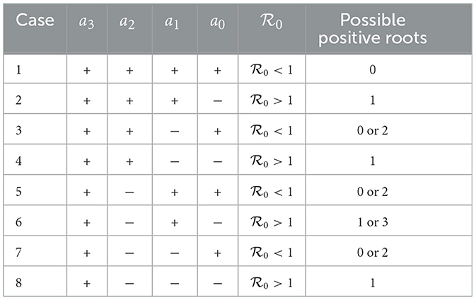
Table 2. The possible number of dengue-endemic equilibria of model (5) depends on whether ${\mathcal{R}}_0$ is lesser or larger than 1.

3.2. Backward bifurcation analysis

In the previous section, we found that the dengue-endemic equilibrium is always locally asymptotically stable if ${\mathcal{R}}_0<1$, and unstable when ${\mathcal{R}}_0>1$. Furthermore, we also found that our simplified IR-model does not always have a unique dengue-endemic equilibrium point. It is possible to have multiple dengue-endemic equilibria when ${\mathcal{R}}_0<1$. Hence, it is important to analyze its local stability criteria. Furthermore, we analyze the bifurcation type of our IR-model using the well-known Castillo–Song bifurcation theorem [54]. The theorem is given as follows.

THEOREM 6 (Castillo–Song Bifurcation Theorem, [54]). Consider a general system of ODEs with parameter ϕ:

$\begin{array}{ll}\frac{dx}{dt}=f(x,\varphi ),f:{ℝ}^n\times ℝ\to {ℝ}^n\text{ and }f\in {ℂ}^2({ℝ}^n\times ℝ).& (16)\end{array}$

Without loss of generality, it is assumed that 0 is an equilibrium of system (16) for all values of the parameter ϕ, that is

$\begin{array}{ll}f(0,\varphi )\equiv 0\text{ for all }\varphi .& (17)\end{array}$

Assume

1. $A=D_{x}f(0,0)=\left(\frac{\partial f_i}{\partial x_j}(0,0)\right)$ is the linearization matrix of system (16) around the equilibrium 0 with ϕ evaluated at 0. Zero is a simple eigenvalue of A and all other eigenvalues of A have negative real parts.

2. Matrix A has a non-negative right eigenvector w and a left eigenvector v corresponding to the zero eigenvalue.

Let f_k be the kth component of f and

$\begin{array}{ll}a={\displaystyle \sum _{k,i,j=1}^n}{v}_k{q}_i{w}_j\frac{{\partial }^2{f}_k}{\partial x_i\partial x_j}(0,0),& (18)\end{array}$

$\begin{array}{ll}b={\displaystyle \sum _{k,i=1}^n}{v}_k{w}_i\frac{{\partial }^2{f}_k}{\partial x_i\partial \varphi }(0,0).& (19)\end{array}$

The local dynamics of (16) around 0 are totally determined by a and b.

1. a > 0, b > 0. When ϕ < 0 with |ϕ| ≪ 1, 0 is locally asymptotically stable, and there exists a positive unstable equilibrium; when 0 < ϕ ≪ 1, 0 is unstable, and there exists a negative and locally asymptotically stable equilibrium;

2. a < 0, b < 0. When ϕ < 0 with |ϕ| ≪ 1, 0 is unstable; when 0 < ϕ ≪ 1, 0 is locally asymptotically stable, and there exists a positive unstable equilibrium;

3. a > 0, b < 0. When ϕ < 0 with |ϕ| ≪ 1, 0 is unstable, and there exists a locally asymptotically stable negative equilibrium; when 0 < ϕ ≪ 1, 0 is stable, and there exists a positive unstable equilibrium;

4. a < 0, b > 0. When ϕ changes from negative to positive, 0 changes its stability from stable to unstable. Correspondingly a negative unstable equilibrium becomes positive and locally asymptotically stable.

Now, we are ready to prove the existence of the backward bifurcation phenomena of our simplified IR-model. Let us assume

$\begin{array}{l}\begin{array}{c}{x}_1=I,x_2=R,\\ g_1=\frac{dI}{dt},g_2=\frac{dR}{dt}.\end{array}\end{array}$

Therefore, the IR-model can be written as

$\begin{array}{l}\begin{array}{c}{g}_1=\frac{{\beta }_h{(1+\alpha x_1)}^2(N-x_1-x_2)x_{1}M}{(1+\alpha x_1)x_1+{\kappa }_v}-(\gamma +{\mu }_h)x_1,\hfill \\ g_2=\gamma x_1-(\delta +{\mu }_h)x_2.\hfill \end{array}\end{array}$

Next, we linearize the above system around the dengue-free equilibrium which yields

$\begin{array}{l}M=\text{J}{|}_{DFE,{\mathcal{R}}_0=1}=\left[\begin{array}{cc}0& 0\\ \gamma & -\delta -{\mu }_h\end{array}\right],\end{array}$

which has two eigenvalues

$\begin{array}{l}{\lambda }_1=0,{\lambda }_2=-\delta -{\mu }_h.\end{array}$

Please note that we have a simple zero eigenvalue, and one other eigenvalue is negative, which fulfills the first assumption of the Castillo–Song bifurcation theorem.

Next, we determine the right eigenvectors of M by solving Mw = 0, where w = (w₁, w₂) is a column vector. We obtained

$\begin{array}{l}{w}_1=\frac{(\delta +{\mu }_h)w_2}{\gamma },w_2=w_2.\end{array}$

Next, we determine the left eigenvectors of M by solving vM = 0, where v = (v₁, v₂) is a row vector. We obtained

$\begin{array}{l}{v}_1=1,v_2=0.\end{array}$

Hence, we have also shown that our preliminary result fulfills two assumptions, such that we can use the Castillo–Song bifurcation theorem.

Next, we calculate a and b using the formula in the Castillo–Song bifurcation theorem. In our case, 0 is the dengue-free equilibrium. We assumed β_h as the bifurcation parameter, such that the critical value of β_h makes ${\mathcal{R}}_0=1$. Since we have that v₂ = 0, there is no need to determine the partial derivatives of g₂. Thus, we had the non-zero derivatives of g₁ as follows:

$\begin{array}{l}\begin{array}{c}\frac{{\partial }^2{g}_1}{\partial x_1^2}(0,0)=\frac{2(\gamma +{\mu }_h)(2N\alpha {\kappa }_v-N-{\kappa }_v)}{N{\kappa }_v},\hfill \\ \frac{{\partial }^2{g}_1}{\partial x_1\partial x_2}(0,0)=-\frac{\gamma +{\mu }_h}{N},\hfill \\ \frac{{\partial }^2{g}_1}{\partial x_2\partial x_1}(0,0)=-\frac{\gamma +{\mu }_h}{N},\hfill \\ \frac{{\partial }^2{g}_1}{\partial x_1\partial {\beta }_h}(0,0)=\frac{NM}{{\kappa }_v}.\hfill \end{array}\hfill \end{array}$

Using the above derivatives, we can obtain the values of a and b as follows:

$\begin{array}{l}\begin{array}{c}a={\displaystyle \sum _{k,i,j=1}^2}{v}_k{w}_i{w}_j\frac{{\partial }^2{g}_k}{\partial x_i\partial x_j}(0,0),\hfill \\ =\frac{2{(\delta +{\mu }_h)}^2(\gamma +{\mu }_h)(2N\alpha {\kappa }_v-N-{\kappa }_v)}{N{\kappa }_v{\gamma }^2}-\frac{2(\delta +{\mu }_h)(\gamma +{\mu }_h)}{\gamma N},\hfill \\ b={\displaystyle \sum _{k,i=1}^2}{v}_k{w}_i\frac{{\partial }^2{g}_k}{\partial x_i\partial {\beta }_h}(0,0),\hfill \\ =\frac{(\delta +{\mu }_h)NM}{\gamma {\kappa }_v}.\hfill \end{array}\hfill \end{array}$

From these calculations, we always obtain b with a positive value, whereas a could be positive or negative. To make a positive, we need to satisfy

$\begin{array}{l}\alpha >\frac{(\gamma +{\mu }_h+\delta ){\kappa }_v+N(\delta +{\mu }_h)}{2(\delta +{\mu }_h)N{\kappa }_v}={\alpha }^{*}.\end{array}$

Hence, we obtained that a is positive when α > α^* and a is negative when α < α^*. Based on the Castillo–Song Theorem, we would have that our IR-model undergoes a forward bifurcation when a is negative and b is positive. On the other hand, we would have that our IR-model undergoes a backward bifurcation when a is positive and b is positive. Hence, our model could undergo backward and forward bifurcation depending on the value of α.

THEOREM 7. Model (5) undergoes a backward bifurcation at ${\mathcal{R}}_0=1$ if α > α^* where

$\begin{array}{l}{\alpha }^{*}=\frac{(\gamma +{\mu }_h+\delta ){\kappa }_v+N(\delta +{\mu }_h)}{2(\delta +{\mu }_h)N{\kappa }_v}.\end{array}$

Otherwise, model (5) undergoes a forward bifurcation when α < α^*.

Please note that α^* in Theorem 7 is the same as with α^* in Theorem 5. The results in this section enumerate some important information from our proposed model.

1. The IR-model in system (5) has a dengue-free equilibrium point. This equilibrium point always exists, and is locally stable if ${\mathcal{R}}_0<1$. These results indicate that we can expect a dengue-free condition in the community as long as we can reduce the basic reproduction number to be <1.

2. The dengue-endemic equilibrium of the IR-model always exists and is locally stable if ${\mathcal{R}}_0>1$. Hence, whenever the dengue-free equilibrium is unstable, we always have a stable endemic equilibrium.

3. It is possible to have a stable endemic equilibrium when ${\mathcal{R}}_0<1$. Hence, a condition ${\mathcal{R}}_0<1$ does not always guarantee the disappearance of dengue from the community.

4. Numerical experiments

In this section, we conduct several numerical experiments to understand the behavior of our model with respect to the level of community ignorance (α). The first simulation will be the bifurcation diagram, followed by numerical simulation on the dynamic of the model with respect to time.

As previously mentioned in Theorem 7, a backward bifurcation occurs when α > α^*, where α presents the ignorance level of the community. Larger α means more ignorance in the community about the spread of dengue. To present the situation, we conduct numerical experiments to show a possible type of bifurcation that could appear from our model. At first, we set up all coefficients on the polynomial (12) as a function of ${\mathcal{R}}_0$. By solving ${\mathcal{R}}_0$ with respect to β_h, we have ${\beta }_h=\frac{(\gamma +{\mu }_h){\kappa }_v{\mathcal{R}}_0}{MN}$, and substituting it in (12), yields:

$\begin{array}{ll}{a}_3({\mathcal{R}}_0)I^3+a_2({\mathcal{R}}_0)I^2+a_1({\mathcal{R}}_0)I+a_0=0,& (20)\end{array}$

where

$\begin{array}{l}{a}_3({\mathcal{R}}_0)={\mathcal{R}}_0\frac{{\kappa }_v(\gamma +{\mu }_h){\alpha }^2(\gamma +{\mu }_h+\delta )}{N},\\ a_2({\mathcal{R}}_0)=-(\alpha (\gamma +{\mu }_h))\\ \frac{{\kappa }_v(N\alpha (\delta +{\mu }_h)-2(\gamma +{\mu }_h+\delta )){\mathcal{R}}_0-N(\delta +{\mu }_h)}{N},\\ a_1({\mathcal{R}}_0)=-(\gamma +{\mu }_h)\\ \frac{{\kappa }_v(2N\alpha ({\mu }_h+\delta )-(\delta +\gamma +{\mu }_h)){\mathcal{R}}_0-N(\delta +{\mu }_h)}{N},\\ a_0({\mathcal{R}}_0)=-(\delta +{\mu }_h)(\gamma +{\mu }_h){\kappa }_v({\mathcal{R}}_0-1).\end{array}$

Next, we substitute the parameter values as given in Section 2.3 which gives us

$\begin{array}{l}0.0196{\mathcal{R}}_0{\alpha }^2{I}^3-(19793{\alpha }^2{\mathcal{R}}_0+(0.039{\mathcal{R}}_0+0.007)\alpha )I^2\dots \end{array}$

$\begin{array}{ll}+(0.007+(0.019-39586\alpha ){\mathcal{R}}_0)I+(19793(1-{\mathcal{R}}_0))=0.& (21)\end{array}$

Using these parameter values, we have the value of α^* as 6.729 × 10⁻⁷. Therefore, we choose α = 5 × 10⁻⁸ < α^* to find the forward bifurcation as shown in Figure 3A and α = 5 × 10⁻⁶ > α^* to find the backward bifurcation as shown in Figure 3B.

FIGURE 3

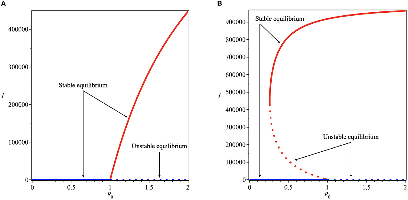
Figure 3. Forward (A) and backward (B) bifurcation diagrams of system (5) for different values of α^*. Red and blue curves present the dengue-free equilibrium and dengue-endemic equilibrium points, respectively.

Backward bifurcation phenomena imply that a condition ${\mathcal{R}}_0<1$ will not be enough to guarantee the disappearance of dengue from the community. We can see that for some parameter value when ${\mathcal{R}}_0<1$, we can have multiple stable equilibrium points, i.e., the dengue-free equilibrium and the endemic equilibrium point (please see Figure 3B). When the ignorance level of the community is small enough (at least smaller than α^*, a condition ${\mathcal{R}}_0<1$ is enough to guarantee the disappearance of dengue from the community (please see Figure 3A). To illustrate the bistability phenomenon when a backward bifurcation appears, we show the phase portrait of system (5) with some initial conditions. The results are given in Figure 4, where we have a stable node dengue-free equilibrium and a stable-spiral endemic equilibrium point. It can be seen that different initial conditions may lead to a different final state condition. To see further impact of α on the bifurcation phenomena of our model, we conduct numerical experiments as shown in Figure 5. These numerical experiments confirm our previous results on the impact of α on the appearance of backward bifurcation phenomena at ${\mathcal{R}}_0=1$. Smaller the level of ignorance of the community, higher the chance to have a free endemic equilibrium when ${\mathcal{R}}_0<1$.

FIGURE 4

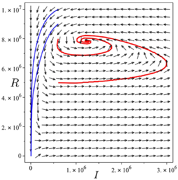
Figure 4. Trajectories of system (5) in I − R plane show bistability phenomena when ${\mathcal{R}}_0=0.5$. Parameter values used are the same as they have been used for Figure 3B. Red curve tends to the endemic equilibrium point, while blue curve tends to the dengue-free equilibrium point.

FIGURE 5

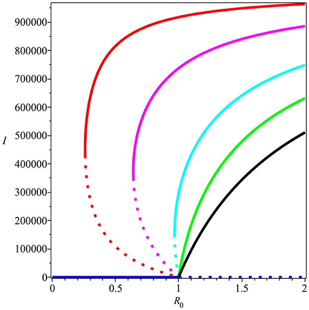
Figure 5. The impact of α on the type of bifurcation phenomena at ${\mathcal{R}}_0=1$. Red, magenta, cyan, green, and black curves present the condition of α being equal to 5, 2, 0.9, 0.5, and 0.2 × 10⁻⁶, respectively.

The public health implication of backward bifurcation is that it is not enough to only reduce the basic reproduction number to eliminate dengue. Another factor, which in our case is the community ignorance level of dengue, should also be considered for further intervention in the field. Therefore, it is necessary to find the impact of model parameters on the critical level of community ignorance. To determine this, we calculate the normalized sensitivity of α^* with respect to γ, μ_h, δ, and κ_v. Using the formula given by [55], we have:

$\begin{array}{l}{\Gamma }_{{\alpha }^{*}}^{\gamma }=\frac{\gamma {\kappa }_v}{N(\delta +{\mu }_h)+{\kappa }_v(\delta +\gamma +{\mu }_h)},\end{array}$

$\begin{array}{l}{\Gamma }_{{\alpha }^{*}}^{{\mu }_h}=-\frac{{\mu }_h{\kappa }_v\gamma }{(\delta +{\mu }_h)(N(\delta +{\mu }_h)+{\kappa }_v(\delta +\gamma +{\mu }_h))}\\ {\Gamma }_{{\alpha }^{*}}^{\delta }=-\frac{\delta {\kappa }_v\gamma }{(\delta +{\mu }_h)(N(\delta +{\mu }_h)+{\kappa }_v(\delta +\gamma +{\mu }_h))}\\ {\Gamma }_{{\alpha }^{*}}^{{\kappa }_v}=-\frac{N(\delta +{\mu }_h)}{N(\delta +{\mu }_h)+{\kappa }_v(\delta +\gamma +{\mu }_h)}.\end{array}$

From a previous analysis, we know that a backward bifurcation will appear when α > α^* and a forward bifurcation if α < α^*. We can see from the expression of ${\Gamma }_{{\alpha }^{*}}$, we have that ${\Gamma }_{{\alpha }^{*}}^{\gamma }>0$, which indicates that increasing γ will increase α^*. Hence, a larger recovery rate will increase the chance of non-appearance of backward bifurcation phenomena at ${\mathcal{R}}_0=1$, since we have a larger interval of α ∈ [0, α^*]. On the other hand, we can see that ${\Gamma }_{{\alpha }^{*}}^{{\mu }_h},{\Gamma }_{{\alpha }^{*}}^{\delta },$ and ${\Gamma }_{{\alpha }^{*}}^{{\kappa }_v}$ are negative, which indicates that increasing natural death rate of human (μ_h), waning immunity (δ), and mosquito dynamic parameters (κ_v) will reduce α^*. Hence, different with the effect of recovery rate, increasing μ_h, δ, and κ_v will increase the chance of appearance of backward bifurcation phenomena, since the interval of α ∈ [0, α^*] is getting smaller. Therefore, we can conclude that longer the temporal immunity of human (smaller δ⁻¹) will increase the chance of finding the only possible condition that dengue disappears when ${\mathcal{R}}_0<1$. Furthermore, we also find that when κ_v increases (larger life expectation of mosquitoes or a smaller infection rate in mosquitoes) will increase the possible existence of dengue-endemic situation in the field, even though ${\mathcal{R}}_0$ is already <1.

Next, we carry out numerical simulation in Figure 6 using MatLab to understand the impact of the human level of ignorance on the spread of dengue. We use the same parameter values that we used to produce Figure 2. We can see that less ignorance of the community (smaller α) to the dynamics of infected individuals will reduce the number of infected individuals. The impact will be more significant as time increases.

FIGURE 6

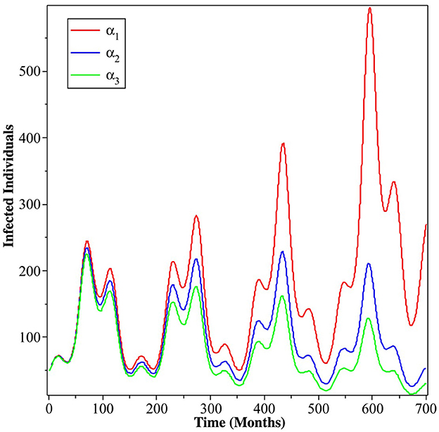
Figure 6. Simulation results showing the impact of the level of ignorance of the community on the dynamics of infected individuals. The red, blue, and green curves present α = 5.1021 × 10⁻⁵, α = 4.1021 × 10⁻⁵, and α = 3.1021 × 10⁻⁵, respectively.

5. Summary and concluding remarks

A mathematical model was presented and studied in this article to assess the impact of the level of human ignorance on the spread of dengue. At the beginning of the study, we introduced our SIR-UV model. Using the QSSA approach, we simplified the model to an IR-model. With this approach, we converted our host–vector dengue model to a host-to-host dengue model. A host-to-host dengue model is a common approach adopted by several researchers to reduce the complexity of their model, by considering the fact that the dynamic of mosquitoes is very fast compared to that of human dynamics [30, 33, 34]. Two types of equilibria emerged from the model, namely the dengue-free equilibrium and the endemic equilibrium point. The basic reproduction number, denoted by ${\mathcal{R}}_0$, was calculated. We found that the dengue-free equilibrium point was always locally asymptotically stable when ${\mathcal{R}}_0<1$. The center manifold theory was used to establish the stability of the endemic equilibrium point, and it showed that the existence of backward bifurcation appears when the level of community ignorance increases. In this situation, we conclude that ensuring the size of the basic reproduction number to be <1 does not always guarantee the disappearance of dengue. Several authors have shown the appearance of a backward bifurcation in the dengue transmission model in their models [56–59]. Their analysis showed that some crucial aspects were not included in the calculation of the basic reproduction number. This aspect may trigger the backward bifurcation phenomena, making the dengue control program more difficult to achieve. In our model, we show that, even though the level of community ignorance does not appear in the basic reproduction number, it does trigger the backward bifurcation. More ignorant the population about dengue, the more difficult it is for dengue to be controlled since the condition of basic reproduction number <1 no longer guarantees the disappearance of dengue.

To test our model, we fit our model output with dengue incidence data in Jakarta, Indonesia. Our preliminary analysis of the time series dengue data reveals the existence of periodicity of dengue incidence data in Jakarta from 2008 to 2021. Three dominant frequencies of the data related to a periodicity of 53, 74, and 147 weeks. These results indicate that dengue cases in Jakarta always recur every year. A numerical experiment on the bifurcation diagram has shown that reducing community ignorance can significantly change the endemic situation. The chance of the existence of dengue-endemic equilibrium when the basic reproduction number is <1 can be avoided when the community ignorance is relatively small. To reduce community ignorance, a media campaign to increase people's awareness of dengue could be an alternative intervention. On the other hand, we find that we can increase the chance of the non-existence of backward bifurcation by increasing the recovery rate of a human, prolonging the temporal immunity, or reducing the life expectancy of a mosquito. Our non-autonomous simulation was conducted by assuming the infection parameter as a sinusoidal function with three dominant frequencies. It has been shown that reducing community ignorance of dengue could suppress the incidence of dengue in Jakarta. Although the outbreak still appears, the outbreak can be reduced significantly. The longer period of intervention of media campaigns to reduce community ignorance will give a more significant reduction in dengue outbreaks.

Data availability statement

The data analyzed in this study is subject to the following licenses/restrictions: It can be available due to personal request to the corresponding author. Requests to access these datasets should be directed to aldiladipo@sci.ui.ac.id.

Author contributions

DA, CA, and RR contributed to the concept and design of the study and wrote the original version of the article. CA organized the data used in the article. DA wrote the final version of the manuscript. All authors contributed to the article and approved the submitted version.

Funding

This research was funded by the Ministry of Education and Culture of Indonesia in collaboration with the Education Fund Management Institution (LPDP) of the Republic of Indonesia through the UKICIS Research Grant Scheme (ID number 4345/E4/AL.04/2022).

Acknowledgments

The authors thank all reviewers for their constructive suggestions.

Conflict of interest

The authors declare that the research was conducted in the absence of any commercial or financial relationships that could be construed as a potential conflict of interest.

Publisher's note

All claims expressed in this article are solely those of the authors and do not necessarily represent those of their affiliated organizations, or those of the publisher, the editors and the reviewers. Any product that may be evaluated in this article, or claim that may be made by its manufacturer, is not guaranteed or endorsed by the publisher.

References

1. World Health Organization (WHO). Dengue and Severe Dengue. (2022). Available online at: https://www.who.int/news-room/fact-sheets/detail/dengue-and-severe-dengue (accessed February 22, 2022).

2. Kraemer MU, Sinka ME, Duda KA, Mylne AQ, Shearer FM, Barker CM, et al. The global distribution of the arbovirus vectors Aedes aegypti and Ae. albopictus. Elife. (2015) 4:e08347. doi: 10.7554/eLife.08347

PubMed Abstract | CrossRef Full Text | Google Scholar

3. Messina JP, Brady OJ, Golding N, Kraemer M, Wint G, Ray SE, et al. The current and future global distribution and population at risk of dengue. Nat Microbiol. (2019) 4:1508–15. doi: 10.1038/s41564-019-0476-8

PubMed Abstract | CrossRef Full Text | Google Scholar

4. Kementerian Kesehatan. Buletin Jendela Epidemiologi, Vol. 2, Agustus 2010. (2010). Available online at: https://www.kemkes.go.id/folder/view/01/structure-publikasi-pusdatin-buletin.html (accessed February 1, 2022).

5. Databox. Musim Penghujan, Terjadi 13.776 Kasus DBD Pada Awal 2022. (2022). Available online at: https://databoks.katadata.co.id (accessed June 15, 2022).

6. Tuiskunen Back A, Lundkvist A. Dengue viruses—an overview. Infect Ecol Epidemiol. (2013) 3:19839. doi: 10.3402/iee.v3i0.19839

PubMed Abstract | CrossRef Full Text

7. Wang E, Ni H, Xu R, Barrett ADT, Watowich SJ, Gubler DJ, et al. Evolutionary relationships of endemic/epidemic and sylvatic dengue viruses. J Virol. (2000) 74:3227–34. doi: 10.1128/jvi.74.7.3227-3234.2000

PubMed Abstract | CrossRef Full Text | Google Scholar

8. Sierra B, Perez AB, Vogt K, Garcia G, Schmolke K, Aguirre E, et al. Secondary heterologous dengue infection risk: disequilibrium between immune regulation and inflammation? Cell Immunol. (2010) 262:134–40. doi: 10.1016/j.cellimm.2010.02.005

PubMed Abstract | CrossRef Full Text | Google Scholar

9. John ALSt, Rathore APS. Adaptive immune responses to primary and secondary dengue virus infections. Nat Rev Immunol. (2019) 19:218–30. doi: 10.1038/s41577-019-0123-x

PubMed Abstract | CrossRef Full Text | Google Scholar

10. Weiskopf D, Sette A. T-cell immunity to infection with dengue virus in humans. Front Immunol. (2014) 5:93. doi: 10.3389/fimmu.2014.00093

PubMed Abstract | CrossRef Full Text | Google Scholar

11. Rothman AL. Cellular immunology of sequential dengue virus infection and its role in disease pathogenesis. In: Ahmed R, Akira S, Casadevall A, Galan JE, Garcia-Sastre A, Mailissen B, Rappuoli R, , editors. Dengue Virus. Berlin; Heidelberg: Springer (2009). p. 83–98.

PubMed Abstract | Google Scholar

12. Guzman MG, Halstead SB, Artsob H, Buchy P, Farrar J, Gubler DJ, et al. Dengue: a continuing global threat. Nat Rev Microbiol. (2010) 8:S7–16. doi: 10.1038/nrmicro2460

PubMed Abstract | CrossRef Full Text | Google Scholar

13. Wilder-Smith A. Dengue vaccine development by the year 2020: challenges and prospects. Curr Opin Virol. (2020) 43:71–8. doi: 10.1016/j.coviro.2020.09.004

PubMed Abstract | CrossRef Full Text | Google Scholar

14. Deng S-Q, Yang X, Wei Y, Chen J-T, Wang X-J, Peng H-J. A review on dengue vaccine development. Vaccines. (2020) 8:63. doi: 10.3390/vaccines8010063

PubMed Abstract | CrossRef Full Text | Google Scholar

15. Zahir A, Ullah A, Shah M, Mussawar A. Community participation, dengue fever prevention and control practices in Swat, Pakistan. Int J MCH AIDS. (2016) 5:39–45. doi: 10.21106/ijma.68

PubMed Abstract | CrossRef Full Text | Google Scholar

16. Kumar N, Verma S, Shiba, Choudhary P, Singhania K, Kumar M. Dengue awareness and its determinants among urban adults of Rohtak, Haryana. J Fam Med Primary Care. 9:2040–4. doi: 10.4103/jfmpc.jfmpc_1203_19

PubMed Abstract | CrossRef Full Text | Google Scholar

17. Rizki LP, Anggreni SN. Community awareness to prevent and control of Dengue fever after Sunda Strait Tsunami in Labuhan, Banten, Indonesia. J Community Med. (2020) 3:1016.

Google Scholar

18. Phuyal P, Kramer IM, Kuch U, Magdeburg A, Groneberg DA, Lamichhane Dhimal M, et al. The knowledge, attitude and practice of community people on dengue fever in Central Nepal: a cross-sectional study. BMC Infect Dis. (2022) 22:454. doi: 10.1186/s12879-022-07404-4

PubMed Abstract | CrossRef Full Text | Google Scholar

19. Aldila D. Dynamical analysis on a malaria model with relapse preventive treatment and saturated fumigation. Comput Math Methods Med. (2022) 2022:1135452. doi: 10.1155/2022/1135452

PubMed Abstract | CrossRef Full Text | Google Scholar

20. Handari BD, Ramadhani RA, Chukwu CW, Khoshnaw SHA, Aldila D. An optimal control model to understand the potential impact of the new vaccine and transmission-blocking drugs for malaria: a case study in Papua and West Papua, Indonesia. Vaccines. (2022) 10:1174. doi: 10.3390/vaccines10081174

PubMed Abstract | CrossRef Full Text | Google Scholar

21. Tasman H, Aldila D, Dumbela PA, Ndii MZ, Herdicho FF, Chukwu CW. Assessing the impact of relapse, reinfection and recrudescence on malaria eradication policy: a bifurcation and optimal control analysis. Trop Med Infect Dis. (2022) 7:263. doi: 10.3390/tropicalmed7100263

PubMed Abstract | CrossRef Full Text | Google Scholar

22. Handari BD, Aldila D, Dewi BO, Rosuliyana H, Khosnaw SHA. Analysis of yellow fever prevention strategy from the perspective of mathematical model and cost-effectiveness analysis. Math Biosci Eng. (2022) 19:1786–824. doi: 10.3934/mbe.2022084

PubMed Abstract | CrossRef Full Text | Google Scholar

23. Aldila D, Rasyiqah K, Ardaneswari G, Tasman H. A mathematical model of Zika disease by considering transition from the asymptomatic to symptomatic phase. J Phys. (2021) 1821:012001. doi: 10.1088/1742-6596/1821/1/012001

CrossRef Full Text | Google Scholar

24. Aldila D. Optimal control for dengue eradication program under the media awareness effect. Int J Nonlin Sci Numer Simul. (2021) 24:95–122. doi: 10.1515/ijnsns-2020-0142

CrossRef Full Text | Google Scholar

25. Ndii MZ. The effects of vaccination, vector controls and media on dengue transmission dynamics with a seasonally varying mosquito population. Results Phys. (2022) 34:105298. doi: 10.1016/j.rinp.2022.105298

CrossRef Full Text | Google Scholar

26. Falcón-Lezama JA, Martínez-Vega RA, Kuri-Morales PA, Ramos-Castañeda J, Adams B. Day-to-day population movement and the management of dengue epidemics. Bull Math Biol. (2016) 78:2011–33. doi: 10.1007/s11538-016-0209-6

PubMed Abstract | CrossRef Full Text | Google Scholar

27. Lourenço J, Recker M. Natural, persistent oscillations in a spatial multi-strain disease system with application to dengue. PLoS Comput Biol. (2013) 9:e1003308. doi: 10.1371/journal.pcbi.1003308

PubMed Abstract | CrossRef Full Text | Google Scholar

28. Gu Y, Khan M, Zarin R, Khan A, Yusuf A, Humphries UW. Mathematical analysis of a new nonlinear dengue epidemic model via deterministic and fractional approach. Alexand Eng J. 67:1–21. doi: 10.1016/j.aej.2022.10.057

CrossRef Full Text | Google Scholar

29. Pandey HR, Phaijoo GR, Gurung DB. Vaccination effect on the dynamics of dengue disease transmission models in Nepal: a fractional derivative approach. Part Differ Equat Appl Math. (2023) 7:100476. doi: 10.1016/j.padiff.2022.100476

CrossRef Full Text | Google Scholar

30. Aguiar M, Stollenwerk N. Mathematical models of dengue fever epidemiology: multi-strain dynamics, immunological aspects associated to disease severity and vaccines. Commun Biomath Sci. (2017) 1:1. doi: 10.5614/cbms.2017.1.1.1

CrossRef Full Text | Google Scholar

31. ten Bosch QA, Singh BK, Hassan MRA, Chadee DD, Michael E. The role of serotype interactions and seasonality in dengue model selection and control: insights from a pattern matching approach. PLoS Negl Trop Dis. (2016) 10:e0004680. doi: 10.1371/journal.pntd.0004680

PubMed Abstract | CrossRef Full Text | Google Scholar

32. Din A, Khan T, Li Y, Tahir H, Khan A, Ali-Khan W. Mathematical analysis of dengue stochastic epidemic model. Results Phys. (2021) 20:103719. doi: 10.1016/j.rinp.2020.103719

CrossRef Full Text | Google Scholar

33. Kabir KA, Tanimoto J. Cost-efficiency analysis of voluntary vaccination against n-serovar diseases using antibody-dependent enhancement: a game approach. J Theor Biol. (2020) 503:110379. doi: 10.1016/j.jtbi.2020.110379

PubMed Abstract | CrossRef Full Text | Google Scholar

34. Aguiar M, Stollenwerk N, Halstead SB. The impact of the newly licensed dengue vaccine in endemic countries. PLoS Negl Trop Dis. (2016) 10:e0005179. doi: 10.1371/journal.pntd.0005179

PubMed Abstract | CrossRef Full Text | Google Scholar

35. Rocha F, Aguiar M, Souza M, Stollenwerk N. Understanding the effect of vector dynamics in epidemic models using center manifold analysis. AIP Conf Proc. (2012) 1479:1319. doi: 10.1063/1.4756398

PubMed Abstract | CrossRef Full Text | Google Scholar

36. Xue L, Zhang H, Sun W, Scoglio C. Transmission dynamics of multi-strain dengue virus with cross-immunity. Appl Math Comput. (2021) 392:125742. doi: 10.1016/j.amc.2020.125742

CrossRef Full Text | Google Scholar

37. Ghosh JK, Ghosh U, Sarkar S. Qualitative analysis and optimal control of a two-strain dengue model with its co-infections. Int J Appl Comput Math. (2020) 6:161. doi: 10.1007/s40819-020-00905-3

CrossRef Full Text | Google Scholar

38. Bock W, Jayathunga Y. Optimal control of a multi-patch Dengue model under the influence of Wolbachia bacterium. Math Biosci. (2019) 315:108219. doi: 10.1016/j.mbs.2019.108219

PubMed Abstract | CrossRef Full Text | Google Scholar

39. Ben-Shachar R, Koelle K. Minimal within-host dengue models highlight the specific roles of the immune response in primary and secondary dengue infections. J R Soc Interface. (2015) 12:20140886. doi: 10.1098/rsif.2014.0886

PubMed Abstract | CrossRef Full Text | Google Scholar

40. Clapham HE, Tricou V, Van Vinh Chau N, Simmons CP, Ferguson NM. Within-host viral dynamics of dengue serotype 1 infection. J R Soc Interface. (2014) 11:20140094. doi: 10.1098/rsif.2014.0094

PubMed Abstract | CrossRef Full Text | Google Scholar

41. Misra AK, Sharma A, Li J. A mathematical model for control of vector borne diseases through media campaigns. Discr Contin Dyn Syst B (2013) 18:1909–27. doi: 10.3934/dcdsb.2013.18.1909

CrossRef Full Text | Google Scholar

42. Mishra A, Gakkhar S. The effects of awareness and vector control on two strains dengue dynamics. Appl Math Comput. (2014) 246:159–67. doi: 10.1016/j.amc.2014.07.115

CrossRef Full Text | Google Scholar

43. Zheng T, Nie L. Modelling the transmission dynamics of two-strain Dengue in the presence awareness and vector control. J Theor Biol. (2018) 443:82–91. doi: 10.1016/j.jtbi.2018.01.017

PubMed Abstract | CrossRef Full Text | Google Scholar

44. Dwivedi A, Keval R. Analysis for transmission of dengue disease with different class of human population. Epidemiol Methods. (2021) 10:20200046. doi: 10.1515/em-2020-0046

CrossRef Full Text | Google Scholar

45. Srivastav AK, Kumar A, Srivastava PK, Ghosh M. Modeling and optimal control of dengue disease with screening and information. Eur Phys J Plus. (2021) 136:1187. doi: 10.1140/epjp/s13360-021-02164-7

PubMed Abstract | CrossRef Full Text | Google Scholar

46. Aldila D, Ndii MZ, Anggriani N, Tasman H, Handari BD. Impact of social awareness, case detection, and hospital capacity on dengue eradication in Jakarta: a mathematical model approach. Alexand Eng J. (2023) 64:691–707. doi: 10.1016/j.aej.2022.11.032

CrossRef Full Text | Google Scholar

47. Alexander ME, Moghadas SM. Bifurcation analysis of an SIRS epidemic model with generalized incidence. SIAM J Appl Math. (2005) 65:1794–816. doi: 10.1137/040604947

PubMed Abstract | CrossRef Full Text | Google Scholar

48. Aldila D, Goetz T, Soewono E. An optimal control problem arising from a dengue disease transmission model. Math Biosci. (2013) 242:9–16. doi: 10.1016/j.mbs.2012.11.014

PubMed Abstract | CrossRef Full Text | Google Scholar

49. Badan Pusat Statistik. Angka Harapan Hidup (AHH) Menurut Provinsi dan Jenis Kelamin Tahun 2018-2020. (2020). Available online at: https://www.bps.go.id/indicator/40/501/1/angka-harapan-hidup-ahh-menurut-provinsi-dan-jenis-kelamin.html (accessed February 18, 2022).

50. Iklim Dan Cuaca Rata-Rata Sepanjang Tahun d Jakarta. Available online at: https://id.weatherspark.com/y/116847/Cuaca-Rata-rata-pada-bulan-in-Jakarta-Indonesia-Sepanjang-Tahun (accessed November 18, 2022).

51. Badan Pusat Statistik. Jumlah Penduduk Provinsi DKI Jakarta Menurut Kelompok Umur dan Jenis Kelamin (Tahun 2018-2020). (2020). Available online at: https://jakarta.bps.go.id/indicator/12/111/1/jumlah-penduduk-provinsi-dki-jakarta-menurut-kelompok-umur-dan-jenis-kelamin.html (accessed February 18, 2022).

52. Wijaya KP, Aldila D, Schafer LE. Learning the seasonality of disease incidences from empirical data. Ecol Complex. (2019) 38:83–97. doi: 10.1016/j.ecocom.2019.03.006

CrossRef Full Text | Google Scholar

53. Diekmann O, Heesterbeek JAP, Roberts MG. The construction of next-generation matrices for compartmental epidemic models. J R Soc Interface. (2010) 7:873–85. doi: 10.1098/rsif.2009.0386

PubMed Abstract | CrossRef Full Text | Google Scholar

54. Castillo-Chavez C, Song B. Dynamical models of tuberculosis and their applications. Math Biosci Eng. (2014) 1:361–404. doi: 10.3934/mbe.2004.1.361

PubMed Abstract | CrossRef Full Text | Google Scholar

55. Chitnis N, Hyman J, Cushing J. Determining important parameters in the spread of malaria through the sensitivity analysis of a mathematical model. Bull Math Biol. (2008) 70:1272–96. doi: 10.1007/s11538-008-9299-0

PubMed Abstract | CrossRef Full Text | Google Scholar

56. Garba SM, Gumel AB, Abu Bakar MR. Backward bifurcations in dengue transmission dynamics. Math Biosci. (2008) 215:11–25. doi: 10.1016/j.mbs.2008.05.002

PubMed Abstract | CrossRef Full Text | Google Scholar

57. Hamdan NI, Kilicman A. The development of a deterministic dengue epidemic model with the influence of temperature: a case study in Malaysia. Appl Math Model. (2021) 90:547–67. doi: 10.1016/j.apm.2020.08.069

CrossRef Full Text | Google Scholar

58. Taghikhani R, Sharomi O, Gumel AB. Dynamics of a two-sex model for the population ecology of dengue mosquitoes in the presence of Wolbachia. Math Biosci. (2020) 328:108426. doi: 10.1016/j.mbs.2020.108426

PubMed Abstract | CrossRef Full Text | Google Scholar

59. Abidemi A, Ackora-Prah J, Fotoyinbo HO, Asamoah JKK. Lyapunov stability analysis and optimization measures for a dengue disease transmission model. Phys A. (2022) 602:127646. doi: 10.1016/j.physa.2022.127646

CrossRef Full Text | Google Scholar