 Arran Hodgkinson
 Aisha Tursynkozha
 Dumitru Trucu
- 1Quantitative Biology and Medicine, Living Systems Institute, University of Exeter, Exeter, United Kingdom
- 2Division of Mathematics, University of Dundee, Dundee, United Kingdom
The eukaryotic cell cycle comprises 4 phases (G1, S, G2, and M) and is an essential component of cellular health, allowing the cell to repair damaged DNA prior to division. Facilitating this processes, p53 is activated by DNA-damage and arrests the cell cycle to allow for the repair of this damage, while mutations in the p53 gene frequently occur in cancer. As such, this process occurs on the cell-scale but affects the organism on the cell population-scale. Here, we present two models of cell cycle progression: The first of these is concerned with the cell-scale process of cell cycle progression and the temporal biochemical processes, driven by cyclins and underlying progression from one phase to the next. The second of these models concerns the cell population-scale process of cell-cycle progression and its arrest under the influence of DNA-damage and p53-activation. Both systems take advantage of structural modeling conventions to develop novels methods for describing and exploring cell-cycle dynamics on these two divergent scales. The cell-scale model represents the accumulations of cyclins across an internal cell space and demonstrates that such a formalism gives rise to a biological clock system, with definite periodicity. The cell population-scale model allows for the exploration of interactions between various regulating proteins and the DNA-damage state of the system and quantitatively demonstrates the structural dynamics which allow p53 to regulate the G2- to M-phase transition and to prevent the mitosis of genetically damaged cells. A divergent periodicity and clear distribution of transition times is observed, as compared with the single-cell system. Comparison to a system with a reduced genetic repair rate shows a greater delay in cell cycle progression and an increased accumulation of cell in the G2-phase, as a result of the p53 biochemical feedback mechanism.
1. Introduction
The healthy functioning of the cell cycle is essential to maintaining the genetic integrity of the cell, protecting it from DNA-damage and becoming a cancer cell, and for the organism's ability to grow and repair itself, in a controlled fashion throughout its lifetime. The eukaryotic cell cycle, in particular, can be split into 4 phases: G1, wherein the cell grows to make space for DNA replication; S, wherein the cell synthesizes a replicate of its DNA; G2, wherein the cell grows once more in preparation for mitosis; and M, wherein the cell splits into two daughter cells, leaving each with a complete set of DNA [1], (see Figure 1A). In order to ensure the healthy progress of the cell cycle, checkpoints at the end of each phase prevent transition to the succeeding phase unless certain biochemical conditions, regulated by a family of proteins called cyclin dependent kinases (CDKs), are met [2]. In general, CDKs remain inactive until their cyclin subunit is bound through the accumulation of cyclins in the cell, throughout the relevant phase of the cell-cycle [3]. These cyclins are typically named after the phase in which they are synthesized (i.e., S-phase cyclins are synthesized in S-phase). Transitions from G1-S and G2-M are controlled by the activation of the CDK protein complex Cdc2:Cdc13 [4], making G1 and G2 escape dependent on similar cyclins.
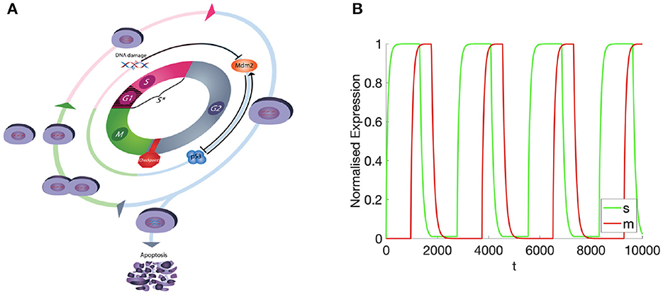
Figure 1. (A) Diagramatic representation of the cell cycle, showing all 4 phases and associated biochemical dynamics accounted for within the model. (B) The masses of M- and S-cyclins over time.
As the biological cell is stressed, either through physical [5], metabolic [6], or chemical [7] mechanisms, DNA-damage may occur and can compromise the healthy functioning of the cell, in situ. In response, the p53 gene is well-established to be activated and, in turn, to activate a plethora of restorative (cell-cycle arrest, DNA-damage repair) or fatal (apoptosis) bio-chemical processes [8, 9]. Consequently, p53 deletions or gain-of-function mutations often lead to cancer or cell death [6, 10–13]. Through the suppression of transcriptional cdc25 activity [14] and additional mechanisms, p53 arrests cell-cycle in the G1 phase [5, 15] in the event of DNA-damage or other cellular stressors. Simultaneously, the synthesized p53 protein promotes the repair of damaged DNA through the induction of O6-methylguanine-DNA methyltransferase [16] and triggers apoptosis in the event that repair fails [17]. Cells in the G1 state are preferentially susceptible to p53-induced cell death [18]. Once DNA-damage has been repaired, it is the role of native levels of the protein mdm2 to degrade p53 [19] and suppress the signal inhibiting cell cycle progression (see Figure 1A). Additional evidence has suggested that p53 may be involved in the regulation of several cell-cycle checkpoints [20], including the G2 cell-cycle checkpoint [14, 15, 21, 22]. Moreover, recent testimony [13] suggests that a population-scale understanding of p53's dynamics is necessary for progress.
Modeling focused on the role of p53 in cell cycle regulation has primarily utilized systems biology or ordinary differential equation (ODE) approaches [23–31], limiting conclusion to the cell scale, where cancer, itself, is a population level phenomenon. The role of p53 in regulating the cell's response to DNA-damage has been explored extensively through analyzes of genetic network dynamics [25–27, 29, 31], demonstrating p53 oscillations and subsequent cell-cycle arrest and/or apoptosis. The role of p53 in cell fate decision-making has been highlighted as a challenge for mathematical biology [28], yet answering this question on the cell-scale, alone, will leave open questions as to the population-scale consequences of these conclusions. In order to expand upon this work, we model cell-scale dynamics using delay integro-differential equations, which allow for inter-temporal biochemical effects of cyclin levels to be accounted for, and population-scale dynamics using partial differential equations (PDEs), which allow for multiple biochemical events to be observed simultaneously at population level.
Early structured approaches to studying cell-cycle dynamics [32] were motivated by the observation that, on the population-scale, cell-cycles were unsynchronised and were unsuited to a mean-field approximation described by singular ODEs. Other structured models of cell-cycle progression have utilized age-size [33, 34] or space-size [35, 36] structured models to track the cell's progression through the cell cycle (as a single quantitative measure of age) to theoretical ends. These models still do not account for the richness and correlation of the interactions between cyclin and DNA-damage states, which would allow for an understanding of how failures in the cell-cycle may contribute to the onset and survival of cancerous cells. One data-inspired, DNA structured approach accounts for the effects of hypoxia on the accumulation of synthesis related DNA-damage in the nucleus [7], demonstrating an application for models of this kind, though without correlating this to the failure of cell-cycle checkpoints. We expand upon previous structured models through a multi-dimensional approach which allows for population-scale cyclin, p53, and mdm2 concentrations to interplay, allowing for a more accurate representation of the biological literature.
To investigate the dynamics of the cell-cycle, we here propose two novel models focussed on cyclin amount and the p53 DNA-repair pathway and its associated mdm2 checkpoint, respectively. The first of these models (Section 2) explores the quantity of S- and M-cyclins across the cell cycle and at the level of the individual cell, through the utilization of a novel, oscillatory PDE framework. The second of these models (Section 3) explores the effect of p53 on DNA-damage repair on the population level, during the course of the cell cycle, using a novel spatio-temporal-structural population level PDE framework similar to that in Domschke et al. [37] and Hodgkinson et al. [38]. To further address the potential role for this model to be used for the simulation of p53 mutant cell lines, relevant in several species of cancer [39], the results for this model (Section 4) are explored across several hypothetical scenarios. The purpose of this study is to explore the dynamics of two fundamentally novel approaches for modeling the cell cycle and to demonstrate their potentials (under a limited parameter set) to give rise to important nonlinearities in cell population-scale behavior.
2. A cell-level model for individual cell-cycle dynamics
As described above, the dynamics involved in the completion of mitosis from a newly birthed daughter cell involve the separation of events across the cell cycle. Presently, we consider a model of a single cell which progresses through the cell cycle, accordingly with their cyclin states which initiate the transition between phases of the cell cycle. Since DNA replication occurs in the S-phase, whilst mitosis occurs in the M-phase, we begin by considering a simple single-cell model consisting of cyclin states for each of these phases, respectively.
2.1. Motivation for the cell-level model
Firstly, since the purpose of this model is to explore the dynamics of the cell cycle within a single-cell, we describe the ‘state’ of the cell based on the relative amounts of the molecules which govern this process; i.e., the total mass of cyclins at time t. For example, the S-cyclin state of the cell describes the relative amounts of S-cyclin in the cell, whilst the overall state of the cell is determined by the relative amounts of S- and M-cyclins or the lack thereof. This state then allows one to determine both the phase of the cell cycle, within which the cell finds itself, and also the trajectory of the cell in time.
Now, let us consider the S-phase of the cell cycle. Allow that all dynamics of this system occur within a time interval, , and an internal cellular spatial domain, , of dimension d with independent variables and (Table 1). Since we are assuming that only S- and M-phase dynamics are relevant for our system, the expression of S-cyclin will necessarily be tied to the activation of the M-phase in the previous cell cycle, such that the S-cyclin state should not increase whenever there are significant numbers of M-cyclins still present within the cell.
Table 1. Table of variables and the domains considered for simulating solutions to Equations (3), (27).
In order to account for the change in the bio-chemistry of the cell, without introducing additional states, we then allow for the existence of a “cellular memory”, whose length is determined by the temporal parameter τ. Biologically, cellular memory can accumulate through the biochemical transformation of a protein's surroundings (for instance, through phosphorylation of target proteins), so that the biochemical landscape of the cell will retain some residual differences from its base state, even after the disappearance of the protein [40, 41]. In this case, and in order to reduce the number of independent variables in the model, we account for this by allowing a delay-intergral in the system of integro-differential equations. In practice, τ serves to determine the time-scale over which the cell may account for its past states while, in theory, this τ represents the time-scale over which the state of a cell will determine its future state, through influencing biochemistry in the present. Thus, we assume that if the historically weighted M-cyclin state, giving rise to current protein levels, is below some critical threshold, θm, then it is assumed that S-cyclin expression will occur, and not in any other case.
Moreover, to account for the fact that cyclins will be produced nearby the nucleus and must diffuse throughout the cell to control whole-cell cell-cycle functioning, we multiply this positive term by appropriate spatial biasing kernel . The purpose of the spatial biasing kernel is to distribute the translation or production of cyclin proteins in the region near to the nucleus and, therefore, we choose the form
Where κp is a decay rate from ξ = 0. Therefore, assuming that the S-cyclin state is normalized and asymptotic to its maximum quantity, the term corresponding to the expression of S-cyclins (i.e., “source of S-cyclins”) within the cell is written as
Where the positivity operator is given by [·]+ : = max(0, ·) and ks > 0 is the cyclin production rate constant.
In simple terms, when m(t, ξ) is sufficiently high across space and some period of time and s(t, ξ) < 1 for p(ξ) > 0, the source term should be positive and S-cyclins are produced. If either of these conditions are not met [i.e., either m(t, ξ) was not sufficiently high for long enough or s(t, ξ) > 1] then the source term will be 0. This acts as a switch to engage production of cyclins and begin the given phase of the cell cycle, just as in the biological case.
Further, the degradation of S-cyclins and subsequent decrease in amount appears, also, to depend upon the M-cyclin state, with S-cyclin being systematically degraded as M-cyclins approach their maximal cellular quantity. Therefore, assume that degradation occurs with a rate μs, we have that the total S-cyclin decay is given by
where
is the usual characteristic function.
On the other hand, exploring now the balance between the source and decay of the M-cyclin population, the relationships between the involved positive and negative terms (of identical form to the ones giving the source and decay for S-cyclins) is here reversed, as M-cyclins are expressed only when historic S-cyclin population levels are above a certain threshold and are degraded only when current S-cyclin states approach their minimum value, 0. Furthermore, both for S- and M- cyclin populations, given that decay toward minimal cyclin quantity is regarded as an exponential asymptotic process, explore this by introducing a parameter ϵ which represents the degree to which levels of cyclin are expected to approach their respective maxima or minima.
Finally, in the presence of the associated balance of source and decay, in order to permeate the entire cell, per unit time, both cyclins populations are assumed to exercise a diffusive spatial transport locally throughout the cyctoplasm, with diffusion coefficients Ds and Dm for S- and M-cyclins, respectively. Hence, the coupled dynamics of S- and M-cyclin populations is therefore given by
Given that these dynamics are assumed to take place within the cyclin-impermeable lipid membrane of the cell and, as such, we impose no flux boundary condition to complete the model.
2.2. Results for the cell-level model
Beginning with initial conditions given by s(0, ξ) = m(0, ξ) = 0 and using a finite differences numerical simulation scheme, alongside central difference calculations for gradient approximation and mid-point integration calculation for integrals, we obtain both spatially and temporally resolved results. As such, we present these firstly as a spatially integrated cyclin state profile over time (Figure 1) and secondly as a time series distributed in the internal cell space, ξ (Figures 2–4). The default parameter set used in this section is given in Table 2.
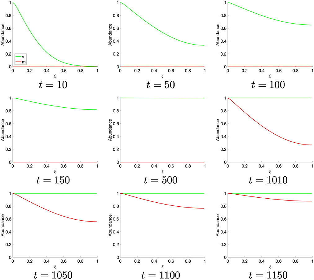
Figure 2. Spatial S- (red) and M- (green) cyclin state estimated for t ∈ [0, 1150].

Table 2. Table of parameters used for simulating solutions to Equation (3).
Observing the temporally resolved data, in the first instance, we find an oscillatory dynamics between the S- and M-cyclin states (Figure 1B). We also observe that the time period over which S-cyclin maintains its near-maximal quantity, |1 − s| < ϵ, is significantly longer than that observed for the M-cyclin, in spite of the controlling variables being equal in value: θm = θs. Also, the relative exclusivity of these two cyclin states means that we can begin to delineate the S- and M-phases, respectively, as those time periods across which either the S- or M- cyclins are at their maximal concentrations, yielding a period of Δt = 2,770.
Let us turn, now, to the spatially resolved system, wherein the S- and M-cyclins are viewed as a time series, as they diffuse through the spatial cell interior, . Beginning at t = 10, we observe the creation of S-cyclins at the origin of the system, ξ = 0, consistently with the cyclin translation (or production) function, p(ξ), followed by the asymptotic homogenisation of the spatial domain through diffusive processes for t ∈ (0,500] (Figure 2). At t ≈ 1,000, the historic activity of S-cyclins becomes sufficient to manifest the process of M-cyclin creation which, again, begins from the origin and homogenizes across the domain as time progresses (Figure 2), such that S- and M-cyclins coexist for some period of time.
At t ≈ 1,310, the population of S-cyclins decreases ubiquitously across the domain as (Figure 3). It may also be readily observed that this process is exponential and asymptotic with s(t, ξ) → 0. Likewise, at t = 1,770, the M-cyclin population begins to decrease ubiquitously in space and exponentially in time, such that m(t, ξ) → 0.
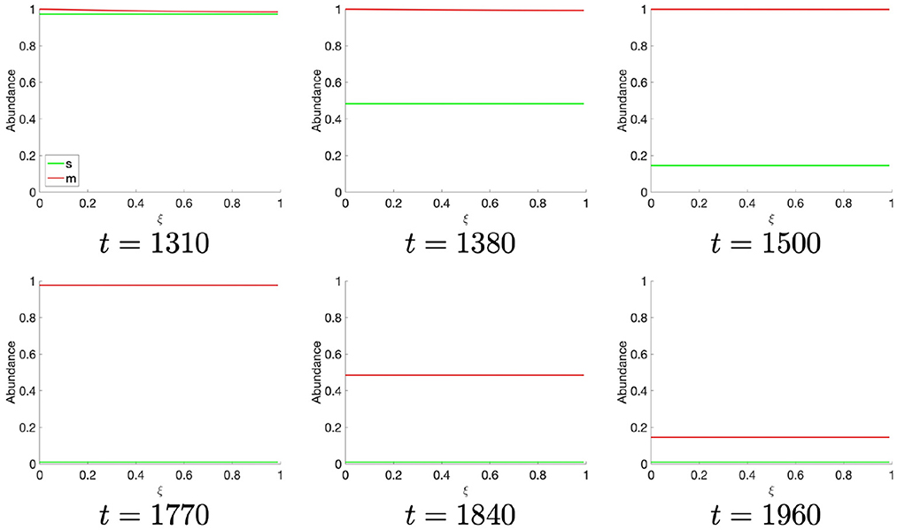
Figure 3. Spatial S- and M-cyclin state estimated for t ∈ [1,310, 1,960].
Comparing this spatial process (Figures 2, 3) with its corresponding temporal process (Figure 1B), we find a close correspondence where the diffusive process accounts for the delay between process initiation and concentration maximization in cyclin states. Moreover, observing the temporal sequence, we find that the S-cyclin state remains significantly greater than 0, whilst the M-cyclin state appears to be at least infinitesimally close to 0. (In fact, since the processes of protein production and protein destruction are both asymptotic, the M-cyclin states may be no less than infinitesimally greater than 0 for times, t′, at which m(t, ξ) > 0 with ). This is due to the assumption that S-cyclins are degraded only for times in which M-cyclins are near-maximal, whilst M-cyclins are degraded where S-cyclin states are near-0, inducing a fundamental asymmetry between these quantities; the time period over which each are degraded is significantly different, under these assumptions and with the given parameter values.
Finally, as the M-cyclin state remains sufficiently low for a sufficient period of time, t ≈ 2, 770, one observes the S-cyclin state begin to rise (Figure 4), similarly as in the above case (Figure 2, t = 10). Likewise, at t ≈ 3, 740 the M-cyclin state again begins to rise and diffuse across the cell to complete the periodic oscillation (Figure 4), correspondingly with the temporal cyclin state data (Figure 1B).
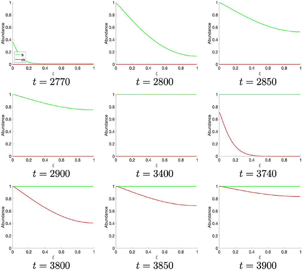
Figure 4. Spatial S- and M-cyclin state estimated for t ∈ [2,770, 3,900].
3. A novel population-level mathematical model for the influence of p53 on cell-cycle dynamics
Having explored a novel model of cell cycling through interdependent oscillations in cyclin expression on the individual cell-level, we now extend the biological context of this model to look at cell population-scale dynamics of cell cycling. Since cyclin expression is the fundamental mode of phase transition across the cell cycle, we retain this dependence through the population-level model. Alongside this dependence on cyclin expression, however, we wish to explore the dynamics of DNA-damage and the critical p53-mdm2 checkpoint in the G2-phase of the cell-cycle. This checkpoint is thought to prevent significantly genetically damaged cells from progressing through to the mitotic, or M-, phase and we shall discuss the assumed dynamics of this checkpoint in detail (Section 3.2).
In order to reconcile the complexity of this cyclin interdependence with a yet more complex model of cell cycle checkpoint operation, however, we simplify the representation of dynamics dependency on cyclin expression. In this population-level model, we assume that cyclin expression increases across the present phase of the cell cycle, whilst transition to the following phase of the cell cycle is probabilistically dependent upon this cyclin expression level. Therefore, no explicit dependence of one cyclin's expression upon the other's need be accounted for. This effectively allows us to extend the cell-level cyclin-dependent cycling model to a population-scale model incorporating additional stochastic dynamics involved in DNA-damage, repair, and biochemical survey.
Firstly, we begin by defining a time interval, , and corresponding independent variable, upon which these dynamics are considered. Next, we define a number of independent variables which mathematically represent the expression levels of S, G, and M-cyclins, respectively, as , , and . In line with this definition, the number of dimensions through which we consider the dynamics of S, G, and M-cyclins are given by ς, γ, ω ∈ ℕ. In our particular case, we consider the simplest case, where ς = γ = ω = 1. In this 1-dimensional case, we consider that there is only one cyclin for any given phase (S, G, or M), whereas the higher dimensional cases, of 2 dimensions or greater, would represent multiple relevant cyclins within a given phase of the cell cycle, which may present with differing biochemical properties and may, for instance, interact with one another. Notable here is that the general model derivation presented below remains valid also in these higher dimensional cases.
Likewise, and across all phases of the cell cycle, we consider that the cells may retain or acquire damage to their genome, which we map onto a ζ−dimensional domain, ζ ∈ ℕ, with an independent variable given by . Meanwhile, the G2-phase checkpoint is mediated by the interaction of p53 and mdm2, whose independent variable are mathematically represented by and , respectively. Likewise, we here consider the 1−dimensional case where ζ = η = δ = 1. The dynamics of each of these essential biochemical properties will be discussed appropriately to motivate modeling construction in Sections 3.1–3.3. Finally, the domains considered here are non-dimensional and are taken as . In practice, this will allow for a simpler interpretation and visualization of results, whilst maintaining the biological realism of the system.
Furthermore, the current model considers the populations of S-, G-, and M-phase cells as mathematically distinct. In particular, , , and represent the cell populations in the S- G-, and M-phases, respectively. The derivation of the fundamental equations governing the temporal-structural dynamics of the S-, G-, and M-phase populations follow the formalism employed in previous studies of cell population dynamics [37, 38].
3.1. S-phase
3.1.1. Derivation of S-phase cell population spatio-temporal dynamics
Given the S-phase population of cells, cs(t, s, z), we begin by considering an arbitrary control volume , with Us and Y assumed to be compact and with piecewise smooth boundaries. Then the total number of cells in Us × Y at a given time t is given by
Using the principle of mass conservation, the change in CUs×Y(t) per unit time in the region Us × Y is given by
where σς−1 and σζ−1 are surface measures on ∂Us and ∂Y respectively and 𝔫(·) is the normal unit vector at a point (·) on the boundary of the corresponding compact set. Moreover, Ss, Fs, and Js are the respective fluxes in source (birth-death processes), S-cyclin concentration, and DNA damage. Supposing now, that Fs and Js are in the C1 class of continuously differentiable vector fields one can use Stokes' Theorem to write
and, using Lebesgue's dominated convergence theorem, one can move the time derivative within the integral for CUs × Y(t) to arrive at
We then use the indicator function to write the equivalent relation in terms of the integral over the ζ + ς−dimensional domain
Then, since we have that Us × Y, where Us and Y are compact with piecewise smooth boundaries is a family of generators for the Borelian σ-algebra on ℝς+ζ, given the density of the simple functions (i.e., finite sums of indicator functions) among the test functions from (i.e., the family smooth compact support functions) in L1 [42], we finally obtain that Equation (8) is valid also in terms of test functions, and so we have that:
where ν(t, s, z) is an arbitrary test function. Thus, we have finally obtained the following general equation, namely:
3.1.2. Defining S-phase flux relations
Firstly, the source-sink function, Ss, will consist of one term accounting for cells which are expected to leave the S-phase of the cell cycle and one for those which are expected to enter it, based on the current state of the system. Cells should exit the S-phase of the cell cycle (to enter the G-Phase) dependent on their S-cyclin state and with a rate of progression, rs. The dependence on cyclin state for cell cycle progression is a function of the cyclin state itself and is described and defined here as , an exponentially decaying function from maximal cyclin levels of 1, given by
where κψ is the probability decay rate from x = 1. Since we define the independent variables to be non-dimensional and contained within the interval [0, 1], this ensures that ψ(1) = 1 whilst 0 ≤ ψ(x) ≤ 1, ∀x ∈ [0, 1). Cells should, then, transition from the M-phase of the cell cycle to the S-phase, dependently with the M-cyclin state of the entering cell, with a rate of progression given by rm and with an S-cyclin distribution given by . The distribution of cell transition to the S-phase are given by the exponentially decaying probability function
where Nσ is a normalization constant and κs is the decay rate of the redistribution function from x = 0. The S-phase source function, as a whole, is then expressed as
We know that S-cyclin state increases over the S-phase, as a marker of S-phase progression. For the S-cyclin flux function, therefore, we assume that the dynamics are composed of both deterministic dynamics toward greater levels of S-cyclin state and random fluctuations in these states. We express the deterministic flux in the form of an advective term toward s = 1, accounting for the normalized domain, with a rate given by χs. The random dynamics in S-cyclin concentrations, on the individual cell-scale, are accounted for through a diffusive term in the S-cyclin domain, on the population-scale, and with a rate given by Ds. The full flux expression is then given by
As for DNA-damage, in line with the majority of the literature in this field [7, 27, 43, 44], we assume this to be an unbiased random process, with time being the only causal factor. In the case of the S-phase, due to the rapid DNA replication which occurs across this phase, we assume that the DNA-damage occurs at some accelerated rate. Therefore, the DNA-damage flux term is expressed as a diffusive dynamic with a generic rate, Dz, plus some additional replicative rate, Dr, such that
3.2. G-phase
Since the derivation of the G-phase dynamics is analogous to that of the S-phase, we begin here simply by stating the fundamental dynamical equation in the G-phase:
As such, the full derivation of the dynamical equation for the G-phase follows that given in Section 3.1.1.
3.2.1. Defining G-phase flux relations
The source term for the cell population in the G-phase is somewhat more complicated than that given in the S-phase due to the increase number of dimensions through which we consider this population. Firstly, the entry of cells to the G-phase arrive exclusively as a result of sufficient S-cyclin state in the S-phase, with the function ψ. Cells are then distributed in (g, p, μ)-components of the G-phase, with σg, σp, σμ. The rate of transition from the S- to the G-phase occurs with a rate rs, where the factor ϕs is utilized to account for the assumed increase of mass, in the population, across the S-phase and is accounted for through during the S- to G-phase transition. In particular, though we assume that the mass of the cell increases across both the S- and G-phases, we utilize ϕs and ϕg (where ϕsϕg = 2) during the transitionary source term, in order to simplify the mathematics and mass-balance. Thus, the total increase in mass of any given cell across the cell cycle will be 2, accounting for the mitosis of the mother cell into 2 daughters of precisely equal mass.
Secondly, the exit of cells from the G-phase depends with ψ on G-cyclin state, with a rate rg. Moreover, since p53 is known to arrest cell cycle progression [15, 20, 21], we assume that the transition of cells from G2- to M-phase is dependent upon the relative amount of p53, as
where Aθ is the magnitude and κθ is decay rate in the distribution from x = 0. Thus, the source term for cells in the S-phase is written as
where the functions ψ, σg, σp, and σμ are the probabilistic transition and distributed source functions defined in Equations (11), (12).
Again, G-cyclin state is known to increase across the G-phase and this is assumed to occur with some regularity, alongside random perturbation. Therefore, we assume a similar form to that taken for the S-phase source but with the corresponding parameterization, χg and Dg, such that
One important dynamic to consider across the G-phase is the p53-mediated checkpoint delay to cell-cycle progression. This occurs primarily through the natural up-regulation of p53 and is mitigated through the subsequent up-regulation of Mdm2, in the absence of DNA-damage, across the same phase of the cell-cycle. In essence, p53 will naturally halt cell-cycle progression, where the concurrent expression of p53 and absence of DNA-damage will allow for Mdm2 expression and a consequent inhibition of p53's effect. In the absence of DNA-damage, therefore, the cell-cycle will be allowed to proceed.
Let us begin by considering the dynamics of p53. As we have observed, we assume that the production of p53 is natural and spontaneous, so that we assume an asymptotic increase in p53 levels from p = 0 to p = 1. We know however, that Mdm2 suppresses this expression of p53 and can mathematically represent this as an asymptotic increase in p53 state from p = 0 to , where μ is the Mdm2 state and ωμ accounts for the fact the form of this inhibitory process is unknown. Therefore, the p53 flux in the G-phase is given by
Similarly, we now consider the Mdm2 flux in the G-phase and begin by acknowledging that this process is dependent upon the state of p53 flux, p. Similarly as with p53, we assume that the Mdm2 state of the cell will increase asymptotically from μ = 0 to μ = 1. In the case of Mdm2, however, we know that DNA-damage, z, exerts an inhibitory effect on the expression of Mdm2 and assume that this will take the form of an asymptotic increase from μ = 0 to , where ωz shall again represent our uncertainty in the form of this inhibitory process. The full Mdm2 flux term is then given by
In both of these cases, it should be noted that the dynamics of the system, as well as the inter-dependence of p53 and Mdm2 will not necessarily cause the population to exhibit any monotonic behavior in either p53 or Mdm2 but will likely exhibit nonlinear behavior. Nevertheless, the value to which the system shall exhibit asymptotic behavior remains accurately described above.
Finally, the DNA-damage during the G-phase shall exhibit 2 primary dynamics; those of random variation and repair. The random variation of the DNA-damage during the G-phase shall exhibit diffusive dynamics with the same generic rate of DNA-damage as can be observed in the S-phase dynamics, although without the additional DNA-damage occurring due to replication. Rather, the G-phase occurs posterior to DNA replication and contains a cell-cycle checkpoint which appears specifically to attempt to mitigate DNA-damage arising during DNA replication. The DNA repair is assumed to cause an exponential decay in the degree of DNA-damage within the cell, with a rate given by χz, such that
note that the efficiency of this DNA repair mechanism shall determine the rate at which the cell population may pass from the G-phase to the M-phase and on to cellular mitosis, controlled by the p53 mechanism. This is the reason for which cells with mutated alleles in p53 often exhibit cancer-like behaviors and unregulated cell-cycle checkpoint control.
3.3. M-phase
Since the derivation of the M-phase dynamics is analogous to that of the S-phase, we begin here simply by stating the fundamental dynamical equation in the M-phase:
As such, the full derivation of the dynamical equation for the M-phase follows that given in Section 3.1.1.
3.3.1. Defining M-phase flux relations
Consistently as defined in the flux relations for the S- and G-phases, the source term in the M-phase is defined based upon the incoming population being distributed with σ in m, yielding
Here, the factor ϕg is utilized to account for the assumed increase of mass, in the population, across the G-phase and is accounted for through during the G- to M-phase transition.
The M-cycling flux in the M-Phase, similarly as in the cases of the S- and G-phase dynamics, are given by both an advective state term and a diffusive random-walk term. The respective parameters for these dynamics, specifically for the M-phase, are given by χm and Dm, respectively. Hence, the M-cyclin flux term is given by
Likewise, the DNA-damage during the M-phase is presumed not to be driven by any particular event but simply by random fluctuation and stochastic interaction of the genome with RNA synthase. Therefore, we assume its dynamics to be governed by a diffusive term with the generic DNA-damage rate, Dz, found in both the S- and G-phases. Hence, the DNA-damage flux is given by
3.4. Full system
Therefore, with all of the individual elements of the model introduced in Equations (10)–(26), the full system of equations for the 3 phasically-resolved subpopulations are given by:
Now that the system, in its entirety, has been derived and discussed, it is useful to consider how various parameters will affect the behavior, dynamics, and outcomes of the system. Firstly, an increase in synthesis rates (χs, χg, and χm) will cause a concurrent increase in the dynamic transition rate of cells to the subsequent phase of the cell cycle, as a result of their accumulation of cyclins and favorable positioning with respect to the relevant ψ. Likewise, an increase in random cyclin fluctuations (Ds, Dg, and Dm) will both cause some cells to defer transition to the subsequent phase and others to transition more rapidly, as a result of the widening distribution in cyclin concentrations.
Now consider the more complicated dynamics of the G2-phase: Firstly, the p53 concentration, p, will increase only with lower levels of p53 and mdm2, μ, since its factor is near-zero for high levels of mdm2. Likewise, the mdm2 concentrations will increase only for low levels of DNA-damage and mdm2, since is near-zero for high levels of DNA-damage. The production of mdm2, however, is also contingent upon the presence of p53. Thus, for high levels of DNA damage, p53 will be produced in the absence of mdm2 until the DNA-damage has been sufficiently repaired, with rate χz, to allow for increases in mdm2 concentration. At such times, p53 production will reverse to a degradative dynamic to allow for p53-dependent transition, with θ(p). Thus, increasing the rates χp or χμ will significantly effect the extent to which this checkpoint operates. For instance, with low χp, one would expect high rates of transition from DNA-damaged cells, due to the lack of p53 to suppress transition. Increasing χμ will likewise admit greater numbers of cells to the subsequent phase due to the increased rate of suppression of p53 in the G2-phase. Consider, also, that an increase in either of the diffusion parameters in the DNA-damage space, Dz and Dr, will therefore cause some subset of cells to remain within the G2-phase for longer, on account of this mdm2-p53 checkpoint.
These inter-phase dynamics yield interesting results for which the trend may be approximated, though the outcome of simultaneously altering multiple parameters may be difficult to predict, a priori. We can also understand general principles of the system, such as that having a greater ϕg, at the expense of ϕs (since ϕsϕg = 2) will allow for a greater efficiency in the system, since biosynthesis is not unnecessarily spent on cells with extensive DNA damage.
4. Computational simulations and results
In order to simulate system (Equation 27), time stepping was achieved using a MacCormack predictor-corrector method and the spatial and structural gradients were calculated using central differences, in the case of diffusion, and downstream differences, in the case of advection. The domains utilized for the simulation of temporal solutions to Equation (27) are normalized and described in Table 1, while the default parameter set utilized is described in Table 3.
Table 3. Table of parameters used for simulating solutions to Equation (27).
In general, the parameters in Table 3 were chosen manually to give rise to a set of clear, and interpretable numerical results. The aim was to demonstrate the dynamics of the system, in this instance, while more rigorous analysis of global robustness and stability falls outside the scope of the current study but remains an open problem. In particular, the default value of diffusion within the system was chosen as 1 × 10⁻² (applying to Dz, Dg, and Dm), since this lies near the upper limit of numerical stability for the parameter. The random DNA damage and S-cyclin fluctuation are lower than the default value to demonstrate a distinction with replicative damage and elongate the S-phase (to account for the absent G1 phase) respectively. Synthesis rates are set to reflect the rapid accumulation of cyclins within the cell, where the effect of changing these values would simply be to alter the dynamic rates of transition, in general. Transition rates (r·), themselves, have been set high in order not to limit the transition of cells but to facilitate their dynamic transition via cyclin accumulation. Finally, form parameters (ωμ and ωz) have been set arbitrarily to 1, whilst κ· parameters and Aθ give rise to sufficiently interesting constraints to allow observation of whole-system dynamics. Other choices for these parameters, and particularly those involving the mdm2-p53 checkpoint, can significantly alter transition rates and, as such, are deserving of further study.
In particular, we simulate two experiments: In the first case, we use the default parameter set (given in Table 3) to simulate a theoretical, healthy cell population before simulating a second population with reduced genetic repair rate (). This serves the purpose of comparison, such that we might understand the dynamics of an unhealthy cell population with respect to its healthy counterpart. In order to fully explicate the dynamics of the system, we separate the description of the system simulated with default parameters into a comparison between phases of the cell-cycle (cs, cg, and cm), prior to conducting a closer examination into the dynamics in the G-phase in particular. This allows for a general understanding of the system to be gained prior to a specific understanding of the p53-mediated G-phase checkpoint.
4.1. Unstructured cell cycle dynamics
In the first instance, we began by simulating the cell cycle by generating solutions to Equation (27), using the given parameters (Table 3), and extracted population level metrics during simulation in MatLab. As expected, cells lost from the 1st cell cycle are incorporated into the second cell cycle, while each cell cycle population exhibits a sigmoidal growth phase before and apparently sub-exponential decay phase (Figure 5A). It is also worth noticing that twice as many cells enter the 2nd cell cycle as have left the 1st so that the population is doubled through a successful mitosis.
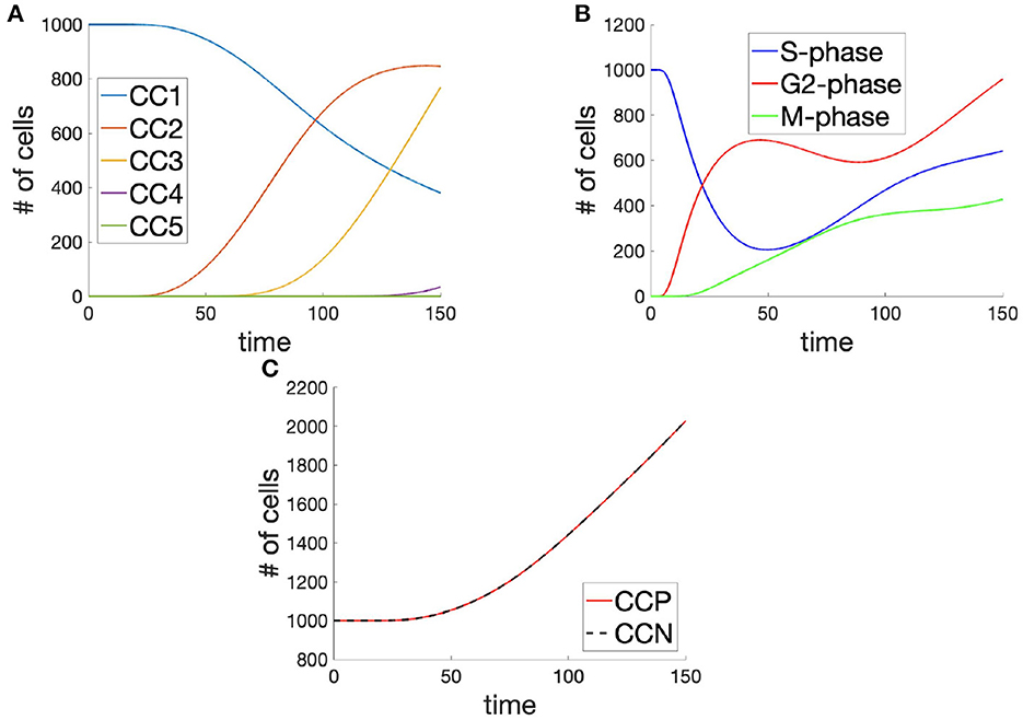
Figure 5. Cell populations (A) in each cell cycle, (B) in each of the phases (across cell cycles), and (C) the total cell population shown as the integral across cell cycle phases (CCP) and cell cycle number (CCN), in time, demonstrating mass-balance between metrics.
Since the processes of the cell cycle are probabilistic, rather than deterministic, and rely on several checkpoints in order to complete a full cycle, the 1st cell cycle still retains a significant percentage of its initial population, even at t = 150. This is despite a speedy and almost complete transition of cells from the S-phase with the time interval t ∈ [0, 100]. In developing organisms, such as Drospohila melanogaster, it is therefore likely that cellular biochemistry is more tightly regulated, in order to achieve the tightly regulated progression of the cycle across the population and the synchronization of mitosis across the embryo during early cycles.
As for the phases of the cell cycle, the entirety of the population originates in the S-phase of the cell cycle, by design (Figure 5B). Although this constitutes a departure from the biological reality of the average system, it allows for a more systematic observation of dynamics and divergence across the system, as a whole. As cells leave the S-phase of the cell cycle, they enter the G2-phase of the cycle and quickly begin to progress through to the M-phase. It is in this G2-phase of the cell cycle that the individual cells, amongst the population can be seen to diverge in their behaviors. Although there exists a significant transfer of cells between the S- and G2-phases, this progresses is arrested in the G2-phase due to the dual requirements of the cell to achieve low levels of DNA-damage and high levels of G-cyclin. This leads to an early onset but slow rate of transfer between the G2- and M-phases of the cell cycle. Cells which do enter the M-phase, however, appear to progress through mitosis successfully and reach their next cell cycle.
Similarly as what is observed in the case of numbered cell cycle populations (Figure 5A), the population is seen to increase at around t = 30 so that the doubling time for the population is given approximately by 150 (Figure 5C). Interestingly, however, the increase in the population has a linear trend, where one might have expected an exponential trend for such a system. Looking back toward the populations within various phases of the cell cycle (Figure 5), it is possible that this linear trend in population growth is explained by the apparently linear trend in the growth of cells within the M-phase, owing to G2-phase checkpoint controls. It is difficult to know whether this relationship does indeed hold in nature or whether the rate of these molecular checkpoints allows for an exponential realization. In order to establish the mass-balance of the cell cycle decomposition approach, we have provided an overlay of the integral across the cell cycle phases, giving the total population, and the sum of the populations across the relevant cell cycles.
4.2. Structured population dynamics
Of course, as is the case in the CDK cell-cycle model, the cell-cycle is characterized by the transition from the S- through the G- to the M-phase biochemistry, where each of these phases are themselves characterized by unique dynamics and cellular behaviors which ultimately result in the growth of the cell population. The progress of the studied cell population through the cell cycle is seen from the decompositions given in Figure 5A, whilst the dynamics of the solutions for the cell population are found in Figures 6–11.
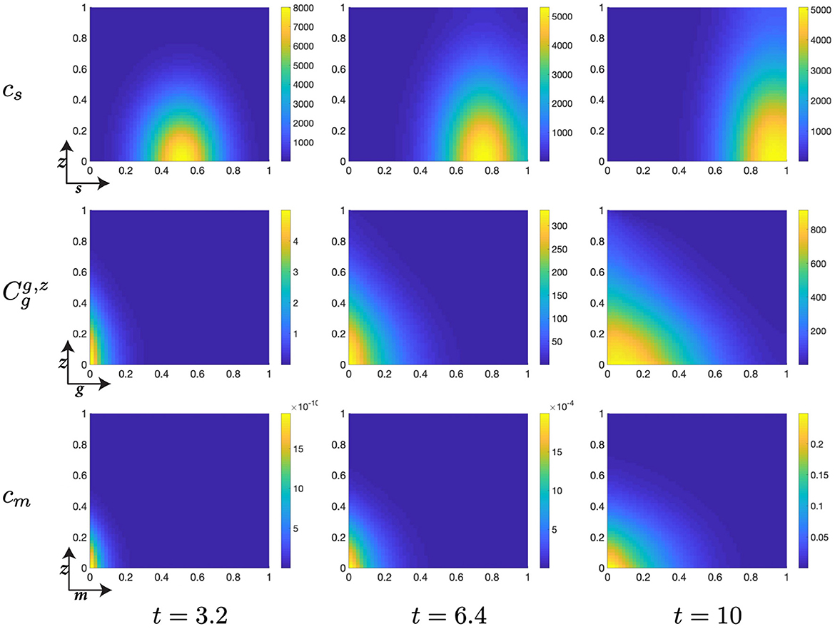
Figure 6. Structured cell populations with S-cyclins (s) and DNA-damage (z), given in the S-phase (cs); G-cyclins (g) and DNA-damage (z), given in the G-phase (); and M-cyclins (m) and DNA-damage (z), given in the M-phase (cm), solved for t ∈ {3.2, 6.4, 10}, respectively.
It is important that one interpret these dynamics carefully, so as to avoid leaving with the mistaken impression that the true nature of the population's dynamics are given explicitly by these solutions to system (Equation 27). Instead, one must bear in mind that these solutions describe density distributions for the population, which must, in turn, be interpreted as a distribution of possible states in which one might expect to find the system. It is the sum of probabilistic expectation functions, across cells, so that each value is the multiple of a population-wide probability density function and the total number of cells at time t. Thus, when small densities are first recorded within the G2 phase, this implies only that there is some non-zero probability that a cell has (or cells have) transitioned into the G2 phase.
As in the case of demographic distributions across a given human population, for example, these density distributions describe the likely characteristics of the populations of a whole, whilst they may fail to describe the precise individual realizations of such a process. For instance, outlier events occur frequently and confound the rationale for such a demographic distribution and, yet, the distribution remains an accurate depiction of the large-scale populations dynamics. Similarly, we here depict the dynamics of the density distribution for entire population, such that fractional elements of cells may transition between phases of the cell cycle, truly representing only a fractional probability that a single whole-cell may have achieved transition across such a boundary. One must appreciate, therefore, that what may be true for the population may still yield surprising results on the individual scale.
4.2.1. Solutions across cell cycle phases
The initial conditions for the cell population in the S-phase are given by a Gaussian distribution in (s, z), centered at (0, 0) and with a standard deviation of 1/20. This crude approximation of the Dirac delta function has the effect of starting the cellular distribution from a well defined position in the domain, such that S-cyclin expression and DNA-damage levels are low, s ≈ 0 and z ≈ 0. Meanwhile, we begin with no cells in the G- or M-phases, such that cg(0, g, p, μ, z) = 0 and cm(0, m, z) = 0.
The early dynamics of the system display a slow but gradual increase in cellular S-cyclin expression, alongside a concurrent increase in DNA-damage levels within the cell (Figure 6). The increase in S-cyclin state within the cell is observed as the migration of the cellular population from initially low values in s to higher values of s across the time interval. Similarly, the increase in DNA-damage levels is observed as the increase in the spread of the population from an initially sharp distribution to a far more dispersed distribution (t = 3.2) along the z-axis. During this time, there exists some small probability that a cell with high S-cyclin state may have transitioned to the G-phase of the cell cycle, which is observed as the distribution arising in the population.
This next time interval sees the critical increase in the number of cells transitioning from the S-phase of the cell cycle to the G-phase (Figure 6, t ∈ [6.4, 10]) and corresponds to the like observation in Figure 5B (red). Given that the S-phase is primarily characterized by the utilization of synthesized biomaterial into the constitutive replication of the eukaryotic chromosome, this introduces a significant degree of DNA-damage in the cell and leads to cells entering the G-phase with a significantly damaged genetic cargo. This is observed as a broad distribution (standard deviation ~ 0.3) along the z-axis at low values of g (g ≈ 0, Figure 6).
The G-phase of the cell cycle is characterized by the initiation of genetic repair and operation of the p53 DNA-damage checkpoint, which should act to prevent sufficiently damaged cells from progressing to the M-phase of the cell cycle. As such we observe that the cell population in the G-phase undergoes a contractile migration from a relatively dispersed population, with respect to DNA-damage levels, at low G-cyclin state, to a collected and narrowly distributed population, with respect to DNA-damage levels, at high G-cyclin state (Figures 6, 7). Across this time interval, t ∈ [10, 30], we also observe the first cells entering the final phase of the cell cycle (M-phase) and can begin to appreciate the extent to which the p53 checkpoint is contributing to the restriction of progress in damaged cells. This manifests through the transition of cells, from the G- to M-phase of the cell cycle, with relatively low levels of DNA-damage. This effect appears to increase in intensity over the passage of time.
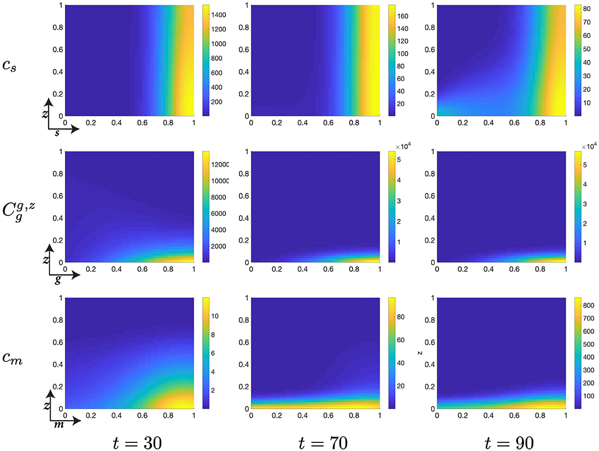
Figure 7. Structured cell populations with S-cyclins (s) and DNA-damage (z), given in the S-phase (cs); G-cyclins (g) and DNA-damage (z), given in the G-phase (); and M-cyclins (m) and DNA-damage (z), given in the M-phase (cm), solved for t ∈ {30, 70, 90}, respectively.
Moreover, during this particular time interval, t ∈ [10, 30] we observe a marked increase in the DNA-damage of cells remaining in the S-phase, as a result of their slow transfer rate to the G-phase of the cell cycle. This concerns the S-phase transition rate, rs, such that for lower values of rs we observe more extensive DNA-damage within the cell. Phenomenologically, this corresponds to the equivalent biological claim that longer DNA duplication inflicts a higher DNA-damage cost to the cell. This increased DNA-damage may also be observed in those cells entering the G-phase but is, nonetheless, resolved through the genetic repair process, prior to entering the M-phase (Figure 7).
As cells migrate through the M-cyclin domain, m, from their initial position, m ≈ 0, to a sufficient expression levels to achieve transition, m ≈ 1, we observe cells beginning to reenter the S-phase and begin their second cell cycle (Figure 7). This can be seen through the manifestations of an additional lobe to the distribution occurring at low values of s and z (Figures 7, 8) and results in a local minimum in the S-phase population (Figure 5B) as it takes on a positive temporal gradient at t ≈ 50. Likewise, we observe that the relatively low values of rs, rg, and rm result in an accumulation of the density distributions at high levels of cyclin state for all phases of the cell cycle (Figure 7), indicating that the probabilistic transition rate, and not cyclin accumulation, is the rate limiting step in our simulated cell population.
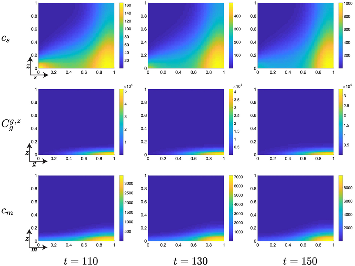
Figure 8. Structured cell populations with S-cyclins (s) and DNA-damage (z), given in the S-phase (cs); G-cyclins (g) and DNA-damage (z), given in the G-phase (); and M-cyclins (m) and DNA-damage (z), given in the M-phase (cm), solved for t ∈ {110, 130, 150}, respectively.
Finally, notice that for higher values of time, t ∈ [50, 150], we observe a significant decrease in the z-directed standard deviation of G-phase distributions, for high cyclin state, g ≈ 1 (Figures 7, 8). This is accompanied by a long residence time for the cell population in the G-phase (observe high cell density levels, Figure 8) and a resultant low-magnitude negative gradient, t ∈ [50, 70], followed by a low-magnitude second temporal derivative, t ∈ [90, 110] in the G-phase population (Figure 5B). This is likely due to the high DNA-damage rate causing low levels of mdm2 expression, resulting in high levels of p53 expression and low effective transition rates from the G- to M-phases of the cell cycle.
To observe the dynamics of the G-phase, we now present identical solutions through multiple dimensions in the G-phase (Section 4.2.2), to increase our ability to scrutinize the dynamics of the G-phase, p53 checkpoint.
4.2.2. Solutions observed within the G2-phase
Our initial conditions are conserved from the above case (Section 4.2.1), such that the G-phase contains 0 cells for t = 0. Solutions for early time points have been omitted on the basis that the G-phase population gains only significant numbers of cells for t ≥ 4.8.
As significant numbers of cells begin to transition from the S- to the G-phase of the cell cycle, we observe that the initial distribution of the population is characterized by a low G-cyclin state, g; a low p53 expression, p; a low mdm2 expression level, μ; and a dispersed DNA-damage level, z, with a standard deviation of ~ 0.3 (Figure 9). The biological significance of the G-phase and, in particular, the p53 checkpoint is to repair those cells with significant DNA-damage and allow only those cells to transition who otherwise possess little damage within their genome. This begins with a steady, unprovoked increase in the expression of p53 within G-phase cells, which can be seen as a migration of the distribution along the p-axis (Figure 9).
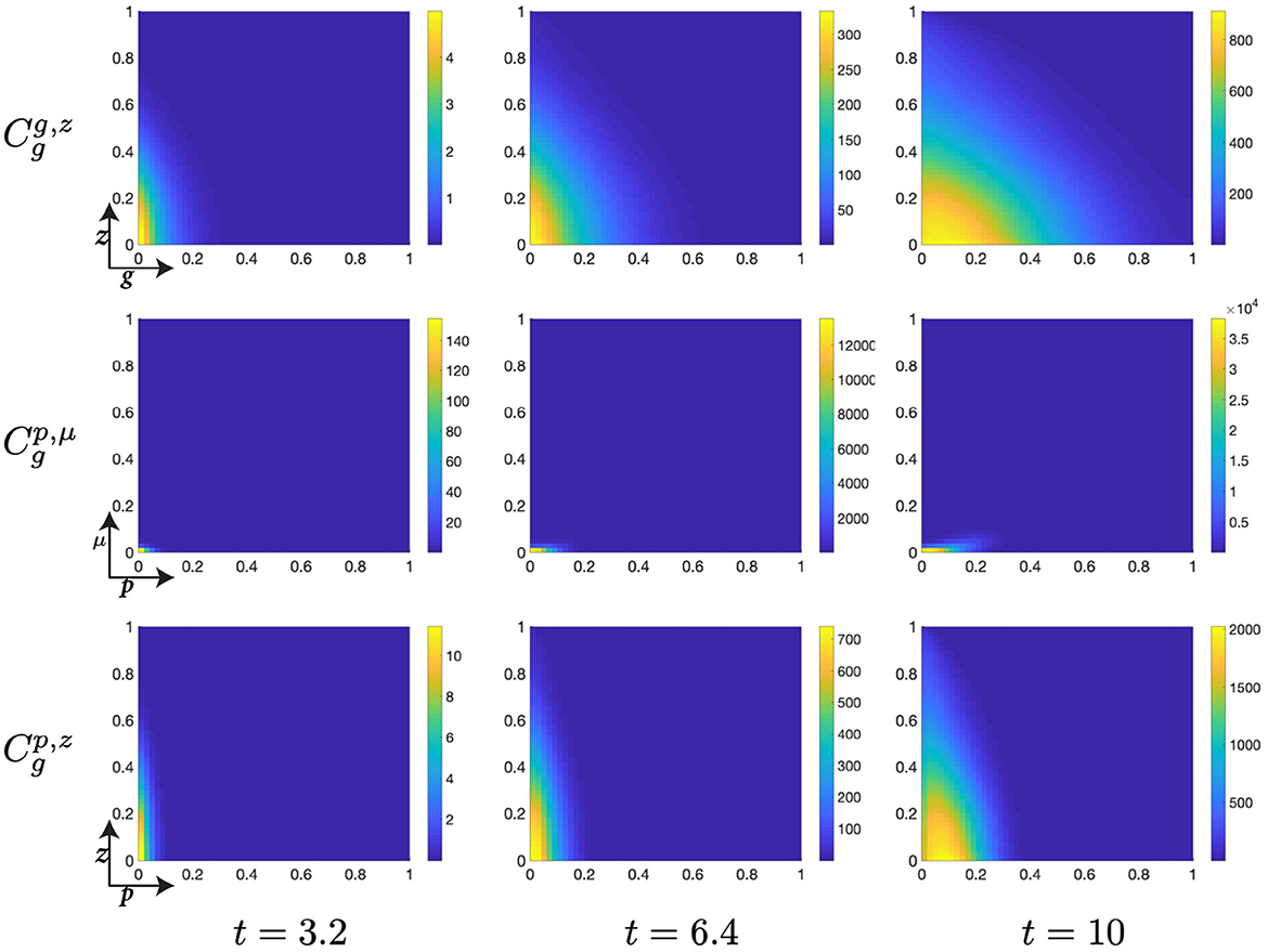
Figure 9. Structured G-phase cell population given in: the G-cyclin-DNA-damage plane (g, z); the p53-mdm2 plane (p, μ); and the p53-DNA-damage plane, solved for t ∈ {3.2, 6.4, 10}, respectively.
Likewise, this phase of the cell cycle is characterized by the ubiquitous search for such genetic abnormalities and their attempted repair, occurring within this mathematical system with the rate χz. Therefore, the longer that cells remain within the G-phase the more of their genome one would expect to have been repaired and the fewer abnormalities they should retain as they progress through their following cycle. Since G-cyclin state is useful as a surrogate measure for residence time within the G-phase, increasing monotonically with residence time, this genetic repair relationship can be seen across the interval where t ∈ [10, 30], since the increase in G-cyclin state is accompanied by a concurrent reduction in the distribution of the population over z (Figures 9, 10).
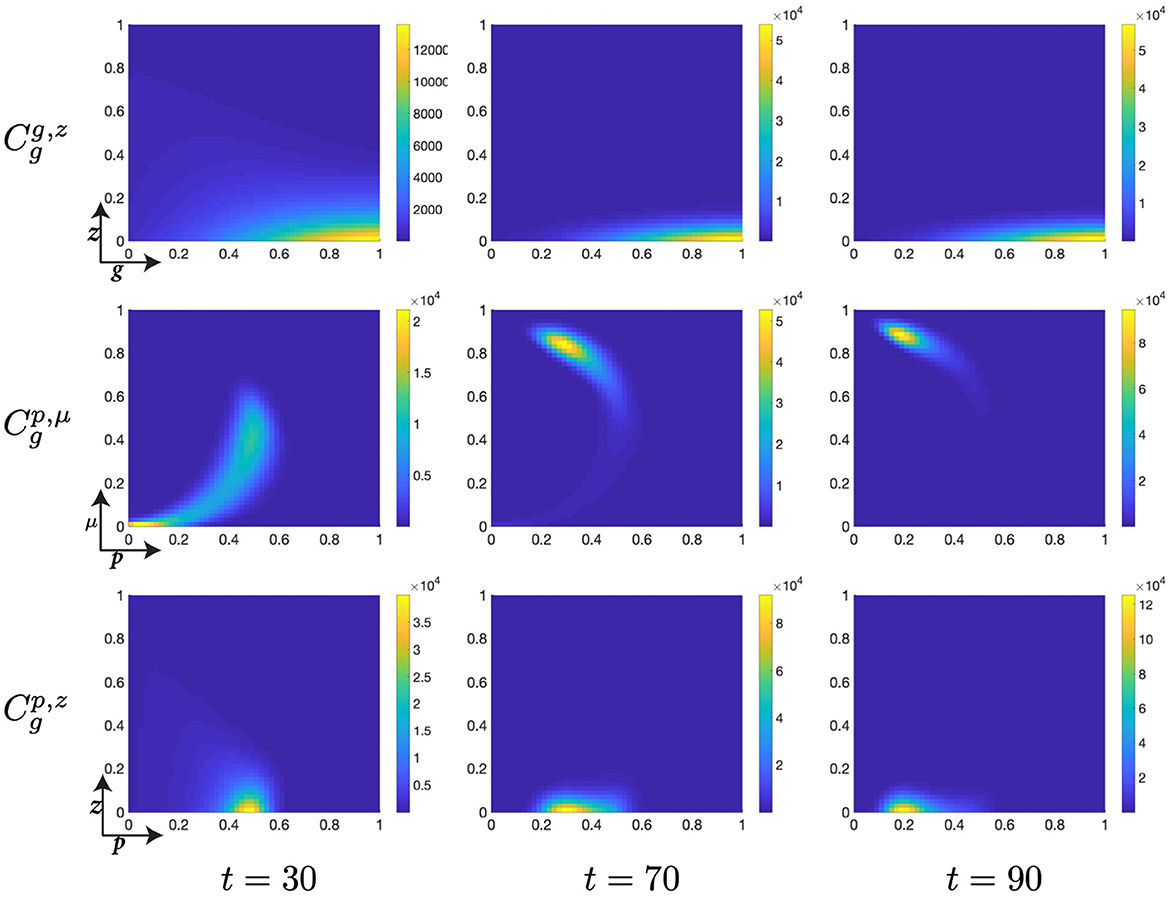
Figure 10. Structured G-phase cell population given in: the G-cyclin-DNA-damage plane (g, z); the p53-mdm2 plane (p, μ); and the p53-DNA-damage plane, solved for t ∈ {30, 70, 90}, respectively.
A similar surrogate measure for residence time (though exclusively at early time points since this relationship is not monotonic) is p53 expression levels. As p53 increases, during the interval t ∈ [10, 30], a clear relationship is observed wherein high levels of p53 expression, p, are accompanied by a narrow distribution in DNA-damage levels, z, whilst low levels of p53 expression are accompanied by a highly distributed population across the DNA-damage spectrum (Figures 9, 10). After this initial period of relative agreement, the cellular distribution begins to exhibit a quadratic form in the (p, μ)-plane, such that the nonlinear increase in Mdm2-expression decreases the rate at which p53-expression increases (Figures 9, 10, , t = 30).
As the cellular population accumulates and consolidates its high levels of G-cyclin expression (Figure 10, ), the nonlinear form of the cellular population through the (p, μ)-plane is completed through a continuing increase in mdm2 expression and the concurrent suppression of p53 expression (Figure 10, ). Simultaneously and by observing the migration of the peaks in the (p, μ)- and (p, z)-planes, we identify that the distribution of cells with reducing p53 expression levels also have significantly reduced DNA-damage levels (Figure 10, ) when compared with the cell population as it initially entered the G-phase (Figure 10, ). As such, we see that the dynamics of the cell cycle are displaying a damaged cell enter the G-phase (after DNA-replication); the cell automatically increases its p53 expression levels; this is met by a repair of the DNA and increase in expression of the healthy DNA reporter, mdm2; which decreases p53 levels and allows transition of the cell to the mitotic phase.
Finally, as p53 levels within the cell decrease and the cellular distribution continues to increase its mean levels of G-cyclin expression (Figure 10), we observe a diminution of the low-p53 high-mdm2 peak (Figure 11) indicating a transition of those cells with repaired DNA out of the G-phase and into the M-phase. This p53-mediated DNA-repair pathway is the rate limiting step in the G-phase transition, illustrated by the early increase in G-cyclin state (Figure 9, ) far in advance of the G-to-M-phase transition. We also observe, over the course of time (Figures 9–11, ) a temporal decrease in the mean and standard deviation in of the cellular distribution in DNA-damage, such that cells at transition exhibit significantly lower DNA-damage than those exhibiting high G-cyclin expression at earlier time points.
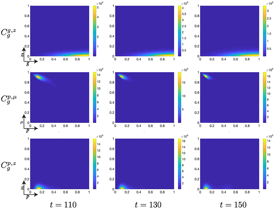
Figure 11. Structured G-phase cell population given in: the G-cyclin-DNA-damage plane (g, z); the p53-mdm2 plane (p, μ); and the p53-DNA-damage plane, solved for t ∈ {110, 130, 150}, respectively.
4.3. Reduced genetic repair rate
Next, in order to investigate the effect of reducing the rate of cell population's intrinsic DNA repair pathway, we re-parameterise the system for χz = 0.02 and observe the change in the underlying structural dynamics in comparison to the above case (Section 4.2.2). During the early stages of simulation (t < 10), results remain qualitatively and quantitatively similar to previous cases and, as such, these results have been omitted for the sake of scientific parsimony.
As significant numbers of cells begin to accumulate within the G-phase of the cell cycle (t ∈ [10, 30]) one observes a significantly increased standard deviation in the DNA-damage spectrum of the cellular population (Figures 12, 13) when comparing to the equivalent population in the previous case (Figures 9, 10). This is to be expected as a result of reducing the DNA-damage repair rate, since χz controls the rate at which the cellular population exhibits asymptotic advection toward z = 0, by definition. On the other hand, the currently considered cellular population (Figures 12, 13, ) exhibits a similar rate of increase in automatic p53 expression across the early stages their G-phase occupation, compared with the previous case (Figures 12, 13, ). Mdm2 expression, as a result of the reduction in DNA-damage repair rate, is, however, limited in this case and transforms the distribution from its previous quadratic form (Figures 12, 13, ) to a far more shallow distribution, exhibiting a form of an order 2 > q > Q polynomial (Figures 12, 13, ), where Q > 2. We must bear in mind that this is a distribution, such that cells exhibit multiple positions upon the (p, μ)-plane which lie between the curves bounded by the order 2 and order Q polynomials.
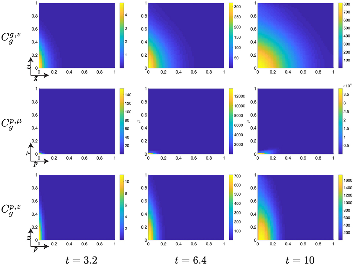
Figure 12. Structured G-phase cell population given in: the G-cyclin-DNA-damage plane (g, z); the p53-mdm2 plane (p, μ); and the p53-DNA-damage plane, with a reduced mutational repair rate () and solved for t ∈ {3.2, 6.4, 10}, respectively.
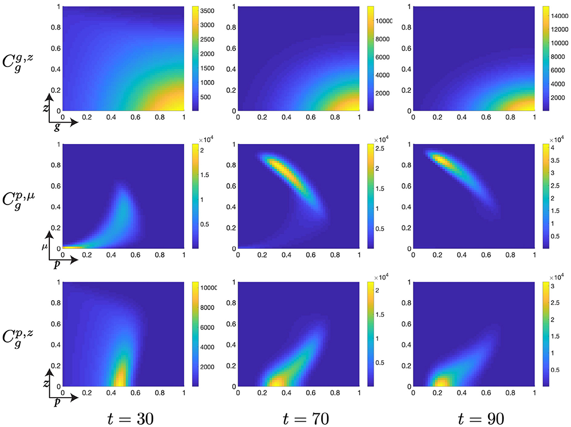
Figure 13. Structured G-phase cell population given in: the G-cyclin-DNA-damage plane (g, z); the p53-mdm2 plane (p, μ); and the p53-DNA-damage plane, with a reduced mutational repair rate () and solved for t ∈ {30, 70, 90}, respectively.
Simultaneously, we begin to observe an increase in the p53 expression levels (Figures 12, 13, ), previously not exceeding p ≈ 0.5 (Figures 12, 13, ), as the DNA-damage levels decrease at a slower rate. During later time points, t ∈ [70, 150], one observes a significant increase in the p53 expression levels in cells with increased residual DNA-damage (Figures 13, 14, ) in comparison cells within the previously considered population (Figures 13, 14, ), who typically underwent DNA-damage repair prior to the occurrence of this increase in p53 expression. Thus, the cellular population appears to mitigate this additional residual DNA-damage by restricting the passage of the cellular population between the G- and M-phases at the G-phase checkpoint.
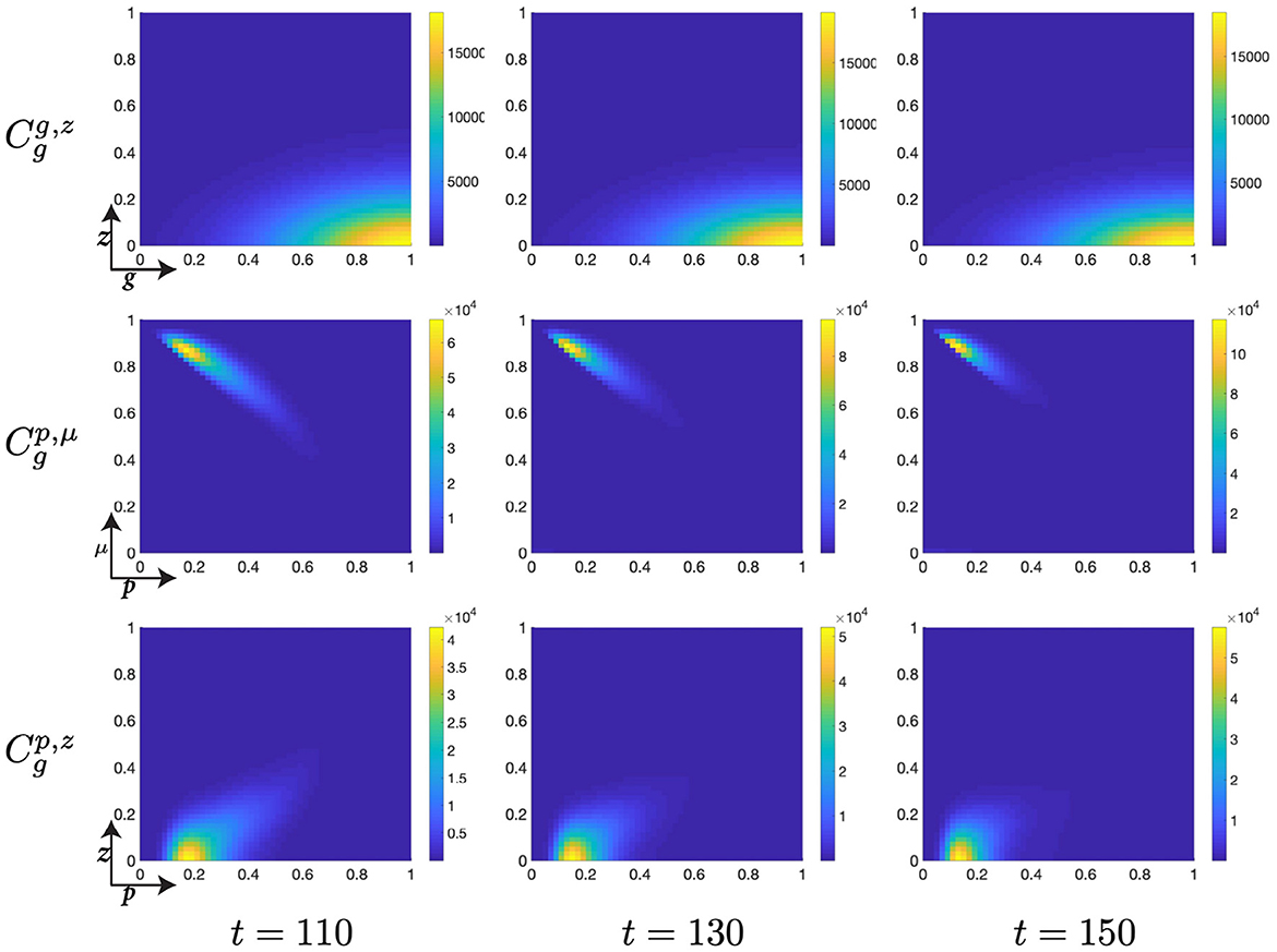
Figure 14. Structured G-phase cell population given in: the G-cyclin-DNA-damage plane (g, z); the p53-mdm2 plane (p, μ); and the p53-DNA-damage plane, with a reduced mutational repair rate () and solved for t ∈ {110, 130, 150}, respectively.
Once again, the cellular distribution for the population with reduced DNA-damage repair rate exhibits a significantly differing profile in the (p, μ)-plane (Figure 13, ) when compared to the previous case (Figure 10, ). In the current case, the distribution is not, in fact, symmetric whilst the previous case shows a reflective symmetric distribution in μ, whilst the additional qualitative comparison on these 2 distributions is left to the reader. Similarly as with the previous case (Figure 11, ), however, we observe that the cell distribution which migrates negatively in p has considerably lower mean DNA-damage levels when compared with the population as a whole (Figure 14, ).
Likewise, across the whole time sequence (Figures 12–14, ), the increase in G-cyclin remains consistent with the previous case (Figures 12–14) whilst the DNA-damage remains elevated, with respect to the standard deviation of the distribution. Notice, further, that the modal DNA-damage is equal in both case, at z = 0, since the DNA-damage mechanism is purely diffusive (such that there exists no mechanism by which this modal value could change). Likewise, even the selective transfer mechanism between the G- and M-phases should ensure that the modal DNA-damage rate within the transferred population remains z = 0. Therefore, to discuss dynamics in the DNA-damage dimension in the case where the initial condition has a modal density at z = 0 is always to speak of the change in the populations distribution through z and not its position in z, per se. This means that although individual cells may change their position with respect to DNA-damage, the most likely situation for a cell is remain without DNA-damage throughout the cell cycle.
5. Discussion and conclusions
We have presented two novel models representing cell-cycle dynamics aiming to highlight different perspectives that the approaches at cell- vs. population- levels can offer in exploring this important process. The first is a single-cell model, wherein the molecular memory of cyclin state triggers discrete transitions between cyclin dynamics and, thus, independent phases of the cell cycle. This model has parallels in gene-protein circadian clock bio-mechanics, for instance in Arabidopsis thaliana [45], and may be relevant to other biological-clock circuits. The second accounted for dynamics across 3 phases of the cell cycle (S, G2, and M), alongside DNA-damage and the p53 pathway for cell-cycle arrest, on the population-scale. Each of these introduce new features to mathematical biology; namely the use and numerical simulation of temporally distributed memory processes, in the first instance, and the interaction between multiple, inter-related structural dimensions, in the second.
Beyond their mathematical significance, the reduction of DNA-damage repair rates in the population-scale model presents a quantitative understanding of how p53 modulates and protects the cell from the propagation of DNA-damage. In the case with reduced repair rate, the model shows a quantitative reduction in the admission of cells into latter phases of the cell-cycle, mediated by the consequent reduction of p53 in cells with an increased extent of DNA-damage. This was observable as a tail in the (p, z)-distribution and a quantitative change in the form of the distribution, in the (p, μ)-plane, which translated to a delayed cell-cycle progression.
The single-cell model allows for a more accurate representation of internal, spatial dynamics which lead to the long-term accumulation of proteins, which triggers the biological transition from S- to M-phase, while the population-scale model allows one to understand the distributed dynamics of stochastic cellular processes, including the p53-mediated arrest of the G2-phase. Though this simulation would not be possible using a deterministic system on the single-cell-scale, since the cell must deterministically transition or fail to do so, a population model allowed for the appreciation of probabilistically distributed cellular dynamics with differing cell-fate outcomes. Likewise, due to computational limitations on the number of dimensions which may be simultaneously simulated at sufficient resolution to allow scientific accuracy, the spatial components of the cell-scale model could not be achieved on the population scale. The development of novel numerical strategies to increase both the resolution and number of dimensions for the simulation of PDEs is, ultimately, both necessary and desirable in order to reconcile this divide.
In other instances, such structured models have been used in conjunction with data. Recently, in Jin et al. [46] and Klowss et al. [47], researchers showed that spatio-temporal models could be used to recapitulate cell-cycle dynamics in spheroid tumors, in vitro. Nonetheless, despite the researchers' descriptions of the spheroid as 4D, constitutively 1-dimensional models were used in these cases. Likewise, models which have used partially structured mathematical models [7], have still not explored the full extent of the biological dynamics which may be captured by such higher-dimensional models as would complement the data. The models presented herein provide an opportunity to researchers to approach the biological description of a given system with a structurally similar mathematical model, simulated in time, space, and structure.
These two new systems present novel methods for modeling biological clocks, though additional work should be conducted to understand the precise nature of these results. Analysis of these systems lies beyond the scope of this initial exploratory research but significant analysis should be undertaken on these systems to determine the underlying mathematical functions driving the observed phenomena. Moreover, a robust set of metrics for this class of model should be set out and utilized for the rigorous comparison between analytic interpretation and numerical simulations, both to visually realize the analytic predictions and to concurrently confirm the validity of the numerical approach, itself.
Data availability statement
The original contributions presented in the study are included in the article/supplementary material, further inquiries can be directed to the corresponding author.
Author contributions
All authors contributed to the manuscript, where AH was primarily responsible for numerical simulations produced in MatLab. All authors contributed to the article and approved the submitted version.
Funding
AH was funded through Wellcome Trust Institution Strategic Support Funding.
Conflict of interest
The authors declare that the research was conducted in the absence of any commercial or financial relationships that could be construed as a potential conflict of interest.
Publisher's note
All claims expressed in this article are solely those of the authors and do not necessarily represent those of their affiliated organizations, or those of the publisher, the editors and the reviewers. Any product that may be evaluated in this article, or claim that may be made by its manufacturer, is not guaranteed or endorsed by the publisher.
References
1. Alberts B, Johnson A, Lewis J, Raff M, Roberts K, Walter P. An overview of the cell cycle. In: Alberts B, Johnson A, Lewis J, Raff M, Roberts K, Walter P, editors. Molecular Biology of the Cell. 4th ed. New York, NY: Garland Science (2002).
2. Cooper GM. The eukaryotic cell cycle. In: Cooper GM, editor. The Cell: A Molecular Approach. 2nd ed. Sunderland, MA: Sinauer Associates (2000).
3. Barnum KJ, O'Connell MJ. Cell cycle regulation by checkpoints. In: Noguchi E, Gadaleta MC, editors. Cell Cycle Control: Mechanisms and Protocols. Vol. 1170 of Methods in Molecular Biology. Sunderland, MA: Springer Science & Business Media (2014).
4. Tyson JJ, Csikasz-Nagy A, Novak B. The dynamics of cell cycle regulation. BioEssays. (2002) 24:1095–109. doi: 10.1002/bies.10191
5. Kuerbitz SJ, Plunkett BS, Walsh WV, Kastan MB. Wild-type p53 is a cell cycle checkpoint determinant following irradiation. Proc Natl Acad Sci USA. (1992) 89:7491–5. doi: 10.1073/pnas.89.16.7491
6. Lahalle A, Lacroix M, De Blasio C, Cissé MY, Linares LK, Le Cam L. The p53 pathway and metabolism: the tree that hides the forest. Cancers. (2021) 13:133. doi: 10.3390/cancers13010133
7. Celora GL, Bader SB, Hammond EM, Maini PK, Pitt-Francis JM, Byrne HM. A DNA-structured mathematical model of cell-cycle progression in cyclic hypoxia. J Theor Biol. (2022) 545:111104. doi: 10.1016/j.jtbi.2022.111104
8. Oren M. Decision making by p53: life, death and cancer. Cell Death Diff. (2003) 10:431–42. doi: 10.1038/sj.cdd.4401183
9. Hafner A, Bulyk ML, Jambhekar A, Lahav G. The multiple mechanisms that regulate p53 activity and cell fate. Nat Rev Mol Cell Biol. (2019) 20:199–210. doi: 10.1038/s41580-019-0110-x
10. Vousden KH, Lu X. Live or let die: the cell's response to p53. Nat Rev Cancer. (2002) 2:594–604. doi: 10.1038/nrc864
11. Liu J, Zhang C, Hu W, Feng Z. Tumor suppressor p53 and its mutants in cancer metabolism. Cancer Lett. (2015) 356:197–203. doi: 10.1016/j.canlet.2013.12.025
12. Chen J. The cell-cycle arrest and apoptotic functions of p53 in tumor initiation and progression. Cold Spring Harbor Perspect Med. (2016) 6:a026104. doi: 10.1101/cshperspect.a026104
13. Lacroix M, Riscal R, Arena G, Linares LK, Le Cam L. Metabolic functions of the tumor suppressor p53: implications in normal physiology, metabolic disorders, and cancer. Mol Metab. (2019) 33:2–22. doi: 10.1016/j.molmet.2019.10.002
14. St Clair S, Giono L, Varmeh-Ziaie S, Resnick-Silverman L, Liu W, Padi A, et al. DNA damage-induced downregulation of Cdc25C Is mediated by p53 via two independent mechanisms: one involves direct binding to the cdc25C promoter. Mol Cell. (2004) 16:725–36. doi: 10.1016/j.molcel.2004.11.002
15. El-Deiry WS. p21/p53, cellular growth control and genomic integrity. In: Vogt PK, Reed SI, editors. Cyclin Dependent Kinase (CDK) Inhibitors. Current Topics in Microbiology and Immunology. Vol. 227. Berlin; Heidelber: Springer (1998).
16. Grombacher T, Eichhorn U, Kaina B. p53 is involved in regulation of the DNA repair gene O6-methylguanine-DNA methyltransferase (MGMT) by DNA damaging agents. Oncogene. (1998) 17:845–51. doi: 10.1038/sj.onc.1202000
17. Lane DP, Lu X, Hupp T, Hall PA. The role of the p53 protein in the apoptotic response. Philos Trans R Soc Lond B. (1994) 345:277–80. doi: 10.1098/rstb.1994.0106
18. Yonish-Rouach E, Grunwald D, Wilder S, Kimchi A, May E, Lawrence JJ, et al. p53-Mediated cell death: relationship to cell cycle control. Mol Cell Biol. (1993) 13:1415–23. doi: 10.1128/mcb.13.3.1415-1423.1993
19. Haupt Y, Mayat R, Kazazt A, Orent M. Mdm2 promotes the rapid degradation of p53. Nature. (1997) 387:296–9. doi: 10.1038/387296a0
20. Giono L, Manfredi JJ. The p53 tumor suppressor participates in multiple cell cycle checkpoints. J Cell Physiol. (2006) 209:13–20. doi: 10.1002/jcp.20689
21. Taylor WR, Stark GR. Regulation of the G2/M transition by p53. Oncogene. (2001) 20:1803–15. doi: 10.1038/sj.onc.1204252
22. Carvajal LA, Hamard PJ, Tonnessen C, Manfredi JJ. E2F7, a novel target, is up-regulated by p53 and mediates DNA damage-dependent transcriptional repression. Genes Dev. (2012) 26:1533–45. doi: 10.1101/gad.184911.111
23. Alarcon T, Byrne HM, Maini PK. A mathematical model of the effects of hypoxia on the cell-cycle of normal and cancer cells. J Theor Biol. (2004) 229:395–411. doi: 10.1016/j.jtbi.2004.04.016
24. Haberichter T, Mädge B, Christopher RA, Yoshioka N, Dhiman A, Miller R, et al. A systems biology dynamical model of mammalian G1 cell cycle progression. Mol Syst Biol. (2007) 3:84. doi: 10.1038/msb4100126
25. Iwamoto K, Hamada H, Eguchi Y, Okamoto M. Mathematical modeling of cell cycle regulation in response to DNA damage: Exploring mechanisms of cell-fate determination. BioSystems. (2011) 103:384–391. doi: 10.1016/j.biosystems.2010.11.011
26. Li Z, Ni M, Li J, Zhang Y, Ouyang Q, Tang C. Decision making of the p53 network: death by integration. J Theor Biol. (2011) 271:205–11. doi: 10.1016/j.jtbi.2010.11.041
27. Chong KH, Samarasinghe S, Kulasiri D. Mathematical modelling of p53 basal dynamics and DNA damage response. Math Biosci. (2015) 259:27–42. doi: 10.1016/j.mbs.2014.10.010
28. Batchelor E, Loewer A. Recent progress and open challenges in modeling p53 dynamics in single cells. Curr Opin Cyctems Biol. (2017) 3:54–9. doi: 10.1016/j.coisb.2017.04.007
29. Chong KH, Samarasinghe S, Kulasiric D, Zheng J. Mathematical modelling of core regulatory mechanism in p53 protein that activates apoptotic switch. J Theor Biol. (2019) 462:134–47. doi: 10.1016/j.jtbi.2018.11.008
30. Heltberg ML, hong Chen S, Jiménez A, Jambhekar A, Jensen MH, Lahav G. Inferring leading interactions in the p53/Mdm2/Mdmx circuit through live-cell imaging and modeling. Cell Syst. (2019) 9:548–558. doi: 10.1016/j.cels.2019.10.010
31. Yang N, Sun T, Shen P. Deciphering p53 dynamics and cell fate in DNA damage response using mathematical modeling. Genome Instabil Dis. (2020) 1:265–77. doi: 10.1007/s42764-020-00019-6
32. Bertuzzi A, Gandolfi A, Giovenco MA. Mathematical models of the cell cycle with a view to tumour studies. Math Biosci. (1981) 53:159–88. doi: 10.1016/0025-5564(81)90017-1
33. Clairambault J, Michel P, Perthame B. A mathematical model of the cell cycle and its circadian control. In: Mathematical Modeling of Biological Systems, Volume I. Boston, MA: Springer (2007). p. 239–51.
34. Pichor K, Rudnicki R. Cell cycle length and long-time behavior of an age-size model. Math Methods Appl Sci. (2022) 45:5797–820. doi: 10.1002/mma.8139
35. Atsou K, Anjuère F, Braud VM, Goudon T. A size and space structured model describing interactions of tumor cells with immune cells reveals cancer persistent equilibrium states in tumorigenesis. J Theor Biol. (2020) 490:110163. doi: 10.1016/j.jtbi.2020.110163
36. Atsou K, Anjuère F, Braud VM, Goudon T. A size and space structured model of tumor growth describes a key role for protumor immune cells in breaking equilibrium states in tumorigenesis. PLoS ONE. (2021) 16:e0259291. doi: 10.1371/journal.pone.0259291
37. Domschke P, Trucu D, Gerisch A, Chaplain MA. Structured models of cell migration incorporating molecular binding processes. J Math Biol. (2017) 75:1517–61. doi: 10.1007/s00285-017-1120-y
38. Hodgkinson A, Uzé G, Radulescu O, Trucu D. Signal propagation in sensing and reciprocating cellular systems with spatial and structural heterogeneity. Bull Math Biol. (2018) 80:1900–36. doi: 10.1007/s11538-018-0439-x
39. Berglind H, Pawitan Y, Kato S, Ishioka C, Soussi T. Analysis of p53 mutation status in human cancer cell lines: a paradigm for cell line cross-contamination mutation status in human cancer cell lines: a paradigm for cell line cross-contamination. Cancer Biol Therapy. (2008) 7:699–708. doi: 10.4161/cbt.7.5.5712
40. Skoge M, Yue H, Erickstad M, Albert Bae A, Levine H, Groisman A, et al. Cellular memory in eukaryotic chemotaxis. Proc Natl Acad Sci USA. (2014) 111:14448–53. doi: 10.1073/pnas.1412197111
41. Cheikhia A, Wallace C, St Croix C, Cohen C, Tang WY, Wipf P, et al. Mitochondria are a substrate of cellular memory. Free Radical Biol Med. (2019) 130:528–41. doi: 10.1016/j.freeradbiomed.2018.11.028
42. Folland GB. Real Analysis : Modern Techniques and Their Applications. 2nd ed. New York, NY: Wiley (1999).
43. Kesseler KJ, Blinov ML, Elston TC, Kaufmann WK, Simpson DA. A predictive mathematical model of the DNA damage G2 checkpoint. J Theor Biol. (2013) 320:159–69. doi: 10.1016/j.jtbi.2012.12.011
44. Barr AR, Cooper S, Heldt FS, Butera F, Stoy H, Mansfeld J, et al. DNA damage during S-phase mediates the proliferation-quiescence decision in the subsequent G1 via p21 expression. Nat Commun. (2017) 8:14728. doi: 10.1038/ncomms14728
45. Pokhilko A, nas Fernández AP, Edwards KD, Southern MM, Halliday KJ, Millar AJ. The clock gene circuit in Arabidopsis includes a repressilator with additional feedback loops. Mol Syst Biol. (2012) 8:574. doi: 10.1038/msb.2012.6
46. Jin W, Spoerri L, Haass NK, Simpson MJ. Mathematical model of tumour spheroid experiments with real-time cell cycle imaging. Bull Math Biol. (2021) 83:44. doi: 10.1007/s11538-021-00878-4
Keywords: cell-cycle, mathematical modeling, cell-scale, cell population scale, temporal-structural dynamics
Citation: Hodgkinson A, Tursynkozha A and Trucu D (2023) Structured dynamics of the cell-cycle at multiple scales. Front. Appl. Math. Stat. 9:1090753. doi: 10.3389/fams.2023.1090753
Received: 06 November 2022; Accepted: 20 February 2023;
Published: 05 April 2023.
Edited by:
Raluca Eftimie, University of Franche-Comté, FranceReviewed by:
Chandrasekhar Venkataraman, University of Sussex, United KingdomDiana Terese White, Clarkson University, United States
Copyright © 2023 Hodgkinson, Tursynkozha and Trucu. This is an open-access article distributed under the terms of the Creative Commons Attribution License (CC BY). The use, distribution or reproduction in other forums is permitted, provided the original author(s) and the copyright owner(s) are credited and that the original publication in this journal is cited, in accordance with accepted academic practice. No use, distribution or reproduction is permitted which does not comply with these terms.
*Correspondence: Dumitru Trucu, dHJ1Y3VAbWF0aHMuZHVuZGVlLmFjLnVr
†Present address: Aisha Tursynkozha, Department of Mathematics, Nazarbayev University, Astana, Kazakhstan