A NSFD method for the singularly perturbed Burgers-Huxley equation

This article focuses on a numerical solution of the singularly perturbed Burgers-Huxley equation. The simultaneous presence of a singular perturbation parameter and the nonlinearity raise the challenge of finding a reliable and efficient numerical solution for this equation via the classical numerical methods. To overcome this challenge, a nonstandard finite difference (NSFD) scheme is developed in the following manner. The time variable is discretized using the backward Euler method. This gives rise to a system of nonlinear ordinary differential equations which are then dealt with using the concept of nonlocal approximation. Through a rigorous error analysis, the proposed scheme has been shown to be parameter-uniform convergent. Simulations conducted on two numerical examples confirm the theoretical result. A comparison with other methods in terms of accuracy and computational cost reveals the superiority of the proposed scheme.

1. Introduction

The time-dependent singularly perturbed Burgers-Huxley equation models a large class of physical phenomena such as the interaction between convection effect, reaction mechanism and diffusion transport. In one dimensional space this equation has the form [1, 2]

$\begin{array}{ll}\{\begin{array}{l}{u}_t-\epsilon u_{xx}+a(u)u_x+b(u)u=0,(x,t)\in D\equiv \Omega \times (0,T]\equiv (0,1)\times (0,T],\\ u(x,0)=u_0(x),x\in \Omega ,\\ u(0,t)=h_1(t),u(1,t)=h_2(t),t\in \left[0,T\right],\end{array}& (1.1)\end{array}$

where

$a(u)=\alpha u,b(u)=-\beta (1-u)(u-\gamma ),$

α ≥ 0, β ≥ 0, γ ∈ (0, 1) are real parameters and u₀(x), h₁(t),and h₂(t) are sufficiently smooth prescribed functions. Here, 0 < ε ≪ 1 denotes the perturbation parameter.

The field of numerical methods for singularly perturbed problems has flourished significantly over the last couple of decades. The studies focused on the design and analysis of numerical methods that were parameter-uniformly convergent. In other words, research was mostly motivated by the challenge posed by the presence of the singular perturbation parameter. A vast majority of researchers discussed linear problems. Nonlinear singularly perturbed equations, and in particular Equation (1.1), received little attention from scholars in this research area. Nonlinearity constitutes an another layer of difficulties of singularly perturbed problems.

In general, the solution of the singularly perturbed Burgers-Huxley problem (1.1) with arbitrary initial and boundary conditions (IBCs) cannot be expressed in terms of a finite number of elementary functions [2, 3]. Thus, several scholars seek approximate analytic solutions using different transformation techniques [4–6]. However, these techniques still hold for only some specific parameters and initial boundary conditions. Hence, for general cases, there is a need to develop numerical methods to obtain an approximate solution of the problem.

For the last two decades, various numerical methods have been studied to solve the Burgers-Huxley equations of type (1.1) for ε = 1 and specific IBCs in the framework of NSFD methods. For example, A.R. Appadu et al. [7] developed two novel nonstandard finite difference schemes, and explicit exponential finite difference method and a fully implicit exponential finite difference method.

For the singularly perturbed case, that is when 0 < ε ≪ 1, various parameter-uniformly convergent methods have been developed to solve (1.1) [1, 2, 8, 9]. It is to be noted that all these works used the Newton's quasilinearization to deal with the nonlinearity.

In this article, a nonstandard finite difference method for the singularly perturbed case is proposed. To deal with the nonlinearity, rather than using quasilinearization, for the first time, nonlinear terms are approximated in a nonlocal manner following one of Micken's rules [10]. The resulting method preserves the properties of the continuous solution and provides reliable numerical results. The method is proved to be first order parameter-uniform convergent in time and space.

The rest of this article is structured in the following manner. In the next section, we study a priori estimates of the analytic solution to the problem. Section 3 is about the proposed NSFD method and its parameter-uniform convergence. Section 4 deals with the implementation of the method to confirm the theoretical results and compare with other methods. Section 5 concludes the present work and provides a direction for future work.

2. Some analytical results: A priori estimates

Throughout this article, we assume that u₀, h₁, and h₂ are sufficiently smooth functions and that a and b satisfy

$\begin{array}{ll}a(u)\ge p>0,b(u)\ge q\ge 0.& (2.1)\end{array}$

Under these assumptions the problem (1.1) has a unique solution $u(x,t)\in C^{2,1}(\bar{D})$ which exhibits a boundary layer near x = 1 [1].

In the rest of the paper, C denotes a generic constant independent of the parameters and mesh sizes, and ||.||_D denotes the maximum norm over D. For the solution u(x, t) of (1.1), we have the following bounds.

Lemma 2.1. [Uniform stability estimate for continuous problem]

Let u(x, t) be the exact solution of (1.1) on $\bar{D}$, then

$||u{||}_{\bar{D}}\le C||u_0{||}_{D_i}+||u{||}_{\partial D},$

where D_i = {(x, t):t = 0, x ∈ [0, 1]}, ∂D = D_i∪D_L∪D_R, D_L = {(x, t):x = 0, t ∈ [0, T]}, and D_R = {(x, t):x = 1, t ∈ [0, T]}.

Proof: The proof can be seen in [9]. □

Remark 2.2. From our assumption in (2.1) and Lemma 2.1, one can observe that the solution u(x, t) satisfies

$\begin{array}{ll}\frac{p}{\alpha }\le u(x,t)\le C||u_0{||}_{D_i}+||u{||}_{\partial D},(x,t)\in \bar{D}.& (2.2)\end{array}$

3. Proposed scheme and its convergence analysis

This section is dedicated to the construction of a new scheme and to the analysis of its parameter-uniform convergence. The first step is to discretize the solution domain $\bar{D}$ and provide the definition of the NSFD methods given in [11] (a revised version of [10]).

Let M and N be positive integers and ${\bar{D}}^{M,N}={\bar{\Omega }}^M\times {\left[0,T\right]}^N$ be uniform grid discretization of the solution domain $\bar{D}=\bar{\Omega }\times \left[0,T\right]$ such that

${\bar{\Omega }}^M=\left\{x_m:x_m=mh,m=0,1,\cdots ,M\right\}$

and

${\left[0,T\right]}^N=\left\{t_n:t_n=n\Delta t,n=0,1,\cdots ,N\right\},$

where h = 1/M and Δt = T/N are spatial and temporal step sizes, respectively.

Definition 3.1. A discrete scheme to determine approximate solutions $u_m^n$ to the solution u(x, t) of the problem (1.1) is called a NSFD method if at least one of the following conditions is satisfied [10]:

1. The classical denominator h or h² of the discrete first or second order derivative is replaced by a nonnegative function ψ such that

$\psi (h)=h+O(h)\text{or }{\psi }^2(h)=h^2+O(h^2).$

For example, denominator functions that satisfy the above conditions are

$\begin{array}{lll}\psi (h)& =h,sin(h),\frac{e^{\beta h}-1}{\beta },\frac{h\epsilon }{a}\left(\text{exp}(\frac{ah}{\epsilon })-1\right)& (3.1)\end{array}$

and so on.

2. Nonlinear terms that occur in the differential equation are approximated in a nonlocal way. For example,

$\begin{array}{l}{u}_m^{n+1}\approx u_m^n,{(u_m^n)}^2\approx u_m^n{v}_{m+1}^n,{(u_m^n)}^2\approx u_m^n\frac{u_{m-1}^n+u_m^n+v_{m+1}^n}{3},\\ {(u_m^{n+1})}^3\approx 2{(u_m^n)}^3-{(u_m^n)}^2{u}_m^{n+1},{(u_m^n)}^3\approx u_{m-1}^n{u}_m^n{u}_{m+1}^n,& (3.2)\end{array}$

and so on.

Definition 3.2. Assume that the solution of (1.1) satisfies some property P. The difference equation of (1.1) in $u_m^n$ is called (qualitatively) stable with respect to P if, for any values of the mesh sizes Δt and h, solution of the difference equation replicates the property P.

Remark 3.3. In [10], Mickens set five rules for the constructions of the finite difference models that can replicate the properties of the exact solution. Definition 3.1 satisfies only two of these rules.

The remaining rules are expressed in terms of definition 3.2. For example, the schemes under consideration in this paper is qualitatively stable with respect to the order of the differential equation, they do satisfy positivity and uniform boundedness.

To construct the scheme, first we semidiscretize the problem (1.1) in time direction and then in space direction.

3.1. Semidiscrete scheme

Denote uⁿ(x) as the approximation of u(x, t_n) at time level t_n, 0 ≤ n ≤ N. Now, we apply backward Euler finite difference method to discretize the continuous problem (1.1) in the temporal direction and obtain the following semidiscrete scheme:

$\begin{array}{ll}\{\begin{array}{l}{u}^0(x)=u(x,0)=u_0(x),\\ (I+\Delta t{{L}}_{\epsilon }^N)u^{n+1}(x)=u^n(x),x\in \Omega ,\\ u^{n+1}(0)=h_1(t_{n+1}),u^{n+1}(1)=h_2(t_{n+1}),n=0,1,\cdots ,N-1,\end{array}& (3.3)\end{array}$

where

${{L}}_{\epsilon }^N\equiv -\epsilon \frac{d^2}{d{x}^2}+a(u^n)\frac{d}{dx}+b(u^n).$

Here the nonlinearity a(u)u_x and b(u)u approximated in a nonlocal way as

$\begin{array}{l}a(u^{n+1})\frac{d{u}^{n+1}}{dx}\approx a(u^n)\frac{d{u}^{n+1}}{dx}\text{and }b(u^{n+1})u^{n+1}\approx b(u^n)u^{n+1}.\end{array}$

and thus this approximation satisfies the condition (2) in definition 3.1.

3.2. Convergence analysis for the semidiscrete scheme

The local truncation error e_n+1 of the semidiscrete scheme (3.3) is given by $e_{n+1}=u(x,t_{n+1})-{û}^{n+1}(x)$, where ûⁿ⁺¹(x) is the solution of

$\begin{array}{ll}\{\begin{array}{l}(I+\Delta t{{L}}_{\epsilon }^N){\widehat{u}}^{n+1}=u(x,t_n),x\in \Omega ,\\ {\widehat{u}}^{n+1}(0)=h_1(t_{n+1}),{\widehat{u}}^{n+1}(1)=h_2(t_{n+1}),n=0,1,\cdots ,N-1.\end{array}& (3.4)\end{array}$

That is, ûⁿ⁺¹(x) is the solution obtained after one step of semidiscrete scheme (3.3) by taking the exact value u(x, t_n) instead of uⁿ(x) as the starting data.

In order to analyze the uniform convergence of the solution uⁿ(x) of (3.3) to the exact solution u(x, t_n), we will perform the stability analysis and establish the consistency result. First, let us consider the semidiscrete maximum principle for the operator $I+\Delta t{{L}}_{\epsilon }^N$.

Lemma 3.4. Let Φⁿ⁺¹(x) be a function such that Φⁿ⁺¹(0) ≥ 0, Φⁿ⁺¹(1) ≥ 0 and $(I+\Delta t{{L}}_{\epsilon }^N){\Phi }^{n+1}(x)\ge 0$ for all x ∈ Ω. Then Φⁿ⁺¹(x) ≥ 0 for all $x\in \bar{\Omega }$.

Proof: Suppose there is $x^{*}\in \bar{\Omega }$ such that ${\Phi }^{n+1}(x^{*})=\underset{x\in \bar{\Omega }}{min}{\Phi }^{n+1}(x)<0.$ From the given hypothesis and second derivative test, we have $x^{*}\ne 0,x^{*}\ne 1,{\Phi }_x^{n+1}(x^{*})=0$ and ${\Phi }_{xx}^{n+1}(x^{*})>0$. Then, from (3.3) we have

$\begin{array}{l}(I+\Delta t{ℒ}_{\epsilon }^N){\Phi }^{n+1}(x^{*})={\Phi }^{n+1}(x^{*})+\Delta t(-\epsilon {\Phi }_{xx}^{n+1}+a({\Phi }^n){\Phi }_x^{n+1}\\ +b({\Phi }^n){\Phi }^{n+1})(x^{*})\\ ={\Phi }^{n+1}(x^{*})+\Delta t(-\epsilon {\Phi }_{xx}^{n+1}(x^{*})\\ +a({\Phi }^n(x^{*})){\Phi }_x^{n+1}(x^{*})+b({\Phi }^n(x^{*})){\Phi }^{n+1}(x^{*}))\\ ={\Phi }^{n+1}(x^{*})+\Delta t(-\epsilon {\Phi }_{xx}^{n+1}(x^{*})\\ +b({\Phi }^n(x^{*})){\Phi }^{n+1}(x^{*})).\end{array}$

Assumption (2.1) leads to $(I+\Delta t{{L}}_{\epsilon }^N){\Phi }^{n+1}(x^{*})<0$, which contradicts the given assumption in Lemma 3.4 and thus Φⁿ⁺¹(x) ≥ 0 for all $x\in \bar{\Omega }$. □

This maximum principle leads to the following stability result

$\begin{array}{ll}||{(I+\Delta t{{L}}_{\epsilon }^N)}^{-1}||\le C.& (3.5)\end{array}$

Lemma 3.5. (Local error estimate)

Estimate of the local error e_n+1 is given by

$\begin{array}{ll}||e_{n+1}||\le C\Delta t^2.& (3.6)\end{array}$

Proof: See [2]. □

The global error E_n+1 associated to the semidiscrete scheme (3.3) at (n+1)-th time level is given by $E_{n+1}=u(x,t_{n+1})-u^{n+1}(x)={\displaystyle \sum _{i=1}^{n+1}}{e}_i$. Using the local error estimate (Lemma 3.5) and triangular inequality the following global error estimate follows.

Theorem 3.6. (Global error estimate)

The global error E_n+1 of the time discretisation at the n + 1 time step satisfies

$\begin{array}{ll}||E_{n+1}||\le C\Delta t,n\Delta t\le T.& (3.7)\end{array}$

Therefore, the semidiscrete scheme (3.3) is a first order uniformly convergent in the time direction.

The following lemma provides the asymptotic estimates of the exact solution uⁿ⁺¹ of (3.3) and its derivatives. These estimates will be used in the convergence analysis of the fully discrete scheme

Lemma 3.7. If uⁿ⁺¹(x) is the solution of the problem (3.3), then there exists a constant C such that

$\begin{array}{ll}||\frac{{\partial }^i{u}^{n+1}}{\partial x^i}{||}_{\bar{\Omega }}\le C\left(1+{\epsilon }^{-i}exp(\frac{-p(1-x)}{\epsilon })\right),0\le i\le 4,\forall x\in \bar{\Omega }.& (3.8)\end{array}$

Proof: See the proof of Lemma 4.1 in [12] □

3.3. The spatial discretisation

In this subsection, we totally discretise the semidiscrete scheme (3.3) on a uniform mesh ${\bar{\Omega }}^M$. Let the approximation of uⁿ(x) at x_m be denoted by $u_m^n$, 0 ≤ m ≤ M. Similarly, let the approximations of $a(u_m^n)$ and $b(u_m^n)$ be denoted respectively by $a_m^n$ and $b_m^n$.

Using the upwind finite difference scheme and nonstandard finite difference methodology of Mickens [13], the semidiscrete problem (3.3) can be fully-discretised as

$\begin{array}{ll}\{\begin{array}{l}(I+\Delta t{{L}}_{\epsilon }^{M,N})u_m^{n+1}=u^n(x_m),1\le m\le M-1,\\ u_0^{n+1}=h_1(t_{n+1}),u_M^{n+1}=h_2(t_{n+1}),\end{array}& (3.9)\end{array}$

where

$\begin{array}{l}{{L}}_{\epsilon }^{M,N}{u}_m^{n+1}\equiv -\epsilon \left[\frac{u_{m+1}^{n+1}-2u_m^{n+1}+u_{m-1}^{n+1}}{{({\psi }_m^n)}^2}\right]+a_m^n\left[\frac{u_m^{n+1}-u_{m-1}^{n+1}}{h}\right]\\ +b_m^n{u}_m^{n+1},\end{array}$

and the denominator function ${\psi }_m^n$ is

${({\psi }_m^n)}^2(h,\epsilon )=\frac{h\epsilon }{a_m^n}\left(\text{exp}(\frac{a_m^{n}h}{\epsilon })-1\right).$

The denominator function is derived systematically to replicate the dissipativity properties of the solution of the differential equations. Interested readers may refer to [14] for details. Observe that

$\begin{array}{l}{({\psi }_m^n)}^2(h,\epsilon )=h^2+O(\frac{h^3}{\epsilon }),\end{array}$

and thus this function satisfies the condition (1) in definition 3.1.

The method in Eq. (3.9) is a linear nonstandard finite difference (LNSFD) and can be written as:

$\begin{array}{ll}{E}_m^{n+1}{u}_{m-1}^{n+1}+F_m^{n+1}{u}_m^{n+1}+G_m^{n+1}{u}_{m+1}^{n+1}=H_m^{n+1},1\le m\le M-1,& (3.10)\end{array}$

where

$\begin{array}{lll}{E}_m^{n+1}& =-\Delta t\left(\frac{\epsilon }{{\left({\psi }_m^n\right)}^2}+\frac{a_m^n}{h}\right),& (3.11)\end{array}$

$\begin{array}{lll}{F}_m^{n+1}& =1+\Delta t\left(\frac{2\epsilon }{{\left({\psi }_m^n\right)}^2}+\frac{a_m^n}{h}+b_m^n\right),& (3.12)\end{array}$

$\begin{array}{lll}{G}_m^{n+1}& =-\frac{\epsilon \Delta t}{{\left({\psi }_m^n\right)}^2},& (3.13)\end{array}$

$\begin{array}{ll}{H}_m^{n+1}& =u_m^n.\end{array}$

Equation (3.10) leads to the tridiagonal system which can be solved with Thomas Algorithm [15, 16].

Remark 3.8. The developed scheme is a linear difference equation even if the original equation (1.1) is nonlinear. This is one of the feature of NSFD.

3.4. Convergence analysis of the space discretisation

The difference operator $I+\Delta t{{L}}_{\epsilon }^{M,N}$ of (3.9) satisfies the following maximum principle. Hence (3.9) has a unique discrete solution $u_m^n$.

Lemma 3.9. Let ${\Phi }_m^{n+1},m=0,1,\cdots ,M$ be fully discrete mesh functions. If ${\Phi }_0^{n+1}\ge 0,{\Phi }_M^{n+1}\ge 0$ and $(I+\Delta t{{L}}_{\epsilon }^{M,N}){\Phi }_m^{n+1}\ge 0$ for 1 ≤ m ≤ M−1 then ${\Phi }_m^{n+1}\ge 0$ for 0 ≤ m ≤ M.

Proof: Let us proof by contradiction. Assume there is m^* such that ${\Phi }_{m^{*}}^{n+1}=\underset{0\le m\le M}{min}{\Phi }_m^{n+1}<0$. Thus, we have, m^*∉{0, M}, ${\Phi }_{m^{*}+1}^{n+1}-{\Phi }_{m^{*}}^{n+1}\ge 0,$ and ${\Phi }_{m^{*}-1}^{n+1}-{\Phi }_{m^{*}}^{n+1}\ge 0.$ Now, from (3.9) we have

$\begin{array}{l}(I+\Delta t{ℒ}_{\epsilon }^{M,N}){\Phi }_{m^{*}}^{n+1}={\Phi }_{m^{*}}^{n+1}+\Delta t[-\epsilon \left(\frac{{\Phi }_{m^{*}+1}^{n+1}-2{\Phi }_{m^{*}}^{n+1}+{\Phi }_{m^{*}-1}^{n+1}}{{({\psi }_{m^{*}}^n)}^2}\right)\\ +a_{m^{*}}^n\left(\frac{{\Phi }_{m^{*}}^{n+1}-{\Phi }_{m^{*}-1}^{n+1}}{h}\right)+b_{m^{*}}^n{\Phi }_{m^{*}}^{n+1}]\\ =-\epsilon \Delta t\left(\frac{{\Phi }_{m^{*}+1}^{n+1}-{\Phi }_{m^{*}}^{n+1}+{\Phi }_{m^{*}-1}^{n-1}-{\Phi }_{m^{*}}^{n+1}}{{({\psi }_{m^{*}}^n)}^2}\right)\\ +a_{m^{*}}^n\Delta t\left(\frac{{\Phi }_{m^{*}}^{n+1}-{\Phi }_{m^{*}-1}^{n+1}}{h}\right)\\ +\left(1+\Delta t{b}_{m^{*}}^n\right){\Phi }_{m^{*}}^{n+1}<0,\\ \end{array}$

which contradicts the given assumption $(I+\Delta t{{L}}_{\epsilon }^{M,N}){\Phi }_m^{n+1}\ge 0$ for 1 ≤ m ≤ M−1 and hence ${\Phi }_m^{n+1}\ge 0$ for 0 ≤ m ≤ M. □

This leads immediately to the following stability result, analogous to the continuous result.

Lemma 3.10. [Uniform stability estimate for discrete problem]

Let ${\Phi }_m^{n+1},0\le m\le M$, be any mesh functions such that ${\Phi }_0^{n+1}={\Phi }_M^{n+1}=0$, then

$|{\Phi }_m^{n+1}|\le \frac{1}{1+q\Delta t}{\displaystyle \underset{1\le i\le M-1}{max}}|(I+\Delta t{{L}}_{\epsilon }^{M,N}){\Phi }_i^{n+1}|,0\le m\le M.$

Proof: Define

${\left[{\text{Ψ}}^{\pm }\right]}_m^{n+1}=\frac{1}{1+q\Delta t}{\displaystyle \underset{1\le i\le M-1}{max}}|(I+\Delta t{{L}}_{\epsilon }^{M,N}){\Phi }_i^{n+1}|\pm {\Phi }_m^{n+1}$

which implies

$\begin{array}{l}{\left[{\Psi }^{\pm }\right]}_0^{n+1}=\frac{1}{1+q\Delta t}\underset{1\le i\le M-1}{\max }|(I+\Delta t{ℒ}_{\epsilon }^{M,N}){\Phi }_i^{n+1}|\pm {\Phi }_0^{n+1}\\ =\frac{1}{1+q\Delta t}\underset{1\le i\le M-1}{\max }|(I+\Delta t{ℒ}_{\epsilon }^{M,N}){\Phi }_i^{n+1}|\ge 0,\\ {\left[{\Psi }^{\pm }\right]}_M^{n+1}=\frac{1}{1+q\Delta t}\underset{1\le i\le M-1}{\max }|(I+\Delta t{ℒ}_{\epsilon }^{M,N}){\Phi }_i^{n+1}|\pm {\Phi }_M^{n+1}\\ =\frac{1}{1+q\Delta t}\underset{1\le i\le M-1}{\max }|(I+\Delta t{ℒ}_{\epsilon }^{M,N}){\Phi }_i^{n+1}|\ge 0,\end{array}$

and, for m = 1, 2, ⋯ , M−1,

$\begin{array}{l}(I+\Delta t{{L}}_{\epsilon }^{M,N}){\left[{\text{Ψ}}^{\pm }\right]}_m^{n+1}=(I+\Delta t{{L}}_{\epsilon }^{M,N})\\ (\frac{1}{1+q\Delta t}{\displaystyle \underset{1\le i\le M-1}{max}}|(I+\Delta t{{L}}_{\epsilon }^{M,N}){\Phi }_i^{n+1}|\pm {\Phi }_m^{n+1})\\ =\frac{1+\Delta t{b}_m^n}{1+q\Delta t}{\displaystyle \underset{0\le m\le M}{max}}|(I+\Delta t{{L}}_{\epsilon }^{M,N}){\Phi }_m^{n+1}|\pm (I+\Delta t{{L}}_{\epsilon }^{M,N}){\Phi }_m^{n+1}.\end{array}$

Since $b^n(x_m)\ge q$, one has $(I+\Delta t{{L}}_{\epsilon }^{M,N}){\left[{\text{Ψ}}^{\pm }\right]}_m^{n+1}\ge 0$. Thus, by discrete maximum principle given in Lemma 3.9, one obtains ${\left[{\text{Ψ}}^{\pm }\right]}_m^{n+1}\ge 0$. This gives the required result

$|{\Phi }_m^{n+1}|\le \frac{1}{q}{\displaystyle \underset{1\le i\le M-1}{max}}|(I+\Delta t{{L}}_{\epsilon }^{M,N}){\Phi }_i^{n+1}|,0\le m\le M.$

□

Remark 3.11. Lemmas 3.9 and 3.10 show the developed nonstandard finite difference method replicates the positivity and boundedness of the solution, respectively. Hence, the proposed method is qualitatively stable.

Theorem 3.12. (Error estimate in the spatial direction)

Let uⁿ⁺¹(x) be the solution of the semidiscrete problem (3.4) and $u_m^{n+1}$ be the solution of the full discretisation (3.9). Then, the error estimate is given by

$|u^{n+1}(x_m)-u_m^{n+1}|\le Ch,0\le m\le M.$

Proof: The truncation error of the complete discretization (3.9) is given by

$\begin{array}{ll}(I+\Delta t{{L}}_{\epsilon }^{M,N})(u^{n+1}(x_m)-u_m^{n+1})& (3.14)\end{array}$

$\begin{array}{l}=\Delta t\left[-\epsilon {\left(u^{n+1}\right)}^{″}\left(x_m\right)+a^n\left(x_m\right){\left(u^{n+1}\right)}^{\prime }\left(x_m\right)+b^n\left(x_m\right)u^{n+1}\left(x_m\right)\right]\\ -\Delta t\left[-\epsilon \frac{h^2}{{\left({\psi }_m^n\right)}^2}{D}^{+}{D}^{-}{u}^{n+1}\left(x_m\right)+a^n\left(x_m\right)D^{-}{u}^{n+1}\left(x_m\right)+b^n\left(x_m\right)u^{n+1}\left(x_m\right)\right]\\ =\epsilon \Delta t\left(\frac{h^2}{{\left({\psi }_m^n\right)}^2}{D}^{+}{D}^{-}-\frac{d^2}{d{x}^2}\right)u^{n+1}\left(x_m\right)+a^n\left(x_m\right)\Delta t\left(\frac{d}{dx}-D^{-}\right)u^{n+1}\left(x_m\right),& (3.15)\end{array}$

where

$\begin{array}{l}{D}^{-}{u}^{n+1}(x_m)=\frac{u^{n+1}(x_m)-u^{n+1}(x_{m-1})}{h},\\ D^{+}{u}^{n+1}(x_m)=\frac{u^{n+1}(x_{m+1})-u^{n+1}(x_m)}{h},\\ D^{+}{D}^{-}{u}^{n+1}(x_m)=\frac{u^{n+1}(x_{m+1})-2u^{n+1}(x_m)+u^{n+1}(x_{m-1})}{h^2}.\end{array}$

Applying absolute values and using triangle inequalities in (3.15) leads to

$\begin{array}{l}\left|(I+\Delta t{ℒ}_{\epsilon }^{M,N})(u^{n+1}(x_m)-u_m^{n+1})\right|\\ \le \epsilon \Delta t\left|(\frac{h^2}{{\left({\psi }_m^n\right)}^2}-1)D^{+}{D}^{-}{u}^{n+1}(x_m)\right|\\ +\epsilon \Delta t\left|(D^{+}{D}^{-}-\frac{d^2}{d{x}^2})u^{n+1}(x_m)\right|\\ +a^n(x_m)\Delta t\left|(\frac{d}{dx}-D^{-})u^{n+1}(x_m)\right|.& (3.16)\end{array}$

From the use the Taylor series expansions of some terms in the above equation, on obtains

$\begin{array}{ll}\frac{h^2}{{\left({\psi }_m^n\right)}^2}-1=-\frac{a^n({\eta }_1)h}{2\epsilon +ha({\eta }_1)},& (3.17)\end{array}$

$\begin{array}{ll}{D}^{+}{D}^{-}{u}^{n+1}(x_m)=\frac{d^2{u}^{n+1}}{d{x}^2}({\eta }_2),& (3.18)\end{array}$

$\begin{array}{ll}(D^{+}{D}^{-}-\frac{d^2}{d{x}^2})u^{n+1}(x_m)=\frac{h^2}{16}\frac{d^4{u}^{n+1}}{d{x}^4}({\eta }_3),& (3.19)\end{array}$

$\begin{array}{ll}(\frac{d}{dx}-D^{-})u^{n+1}(x_m)=\frac{h}{2}\frac{d^2{u}^{n+1}}{d{x}^2}({\eta }_4),& (3.20)\end{array}$

for some η_i such that x_m−1 ≤ η_i ≤ x_m+1, i = 1, 2, 3, 4.

Substituting equations (3.17)–(3.20) in (3.16) and from the boundedness of aⁿ(x) in (3.8), one has

$\begin{array}{l}\left|(I+\Delta t{ℒ}_{\epsilon }^{M,N})(u^{n+1}(x_m)-u_m^{n+1})\right|\le \epsilon \Delta t\frac{a^n({\eta }_1)h}{2\epsilon +h{a}^n({\eta }_1)}|\frac{d^2{u}^{n+1}}{d{x}^2}({\eta }_2)|\\ +\epsilon \Delta t\frac{h^2}{16}|\frac{d^4{u}^{n+1}}{d{x}^4}({\eta }_3)|\\ +a^n(x_m)\Delta t\frac{h}{2}|\frac{d^2{u}^{n+1}}{d{x}^2}({\eta }_4)|,& (3.21)\end{array}$

and this gives

$\begin{array}{l}\left|(I+\Delta t{ℒ}^{M,N})(u^{n+1}(x_m)-u_m^{n+1})\right|\\ \le Ch\left(1+{\epsilon }^{-2}\exp (\frac{-p(1-x_m)}{\epsilon })\right)\\ +C{h}^2\left(\epsilon +{\epsilon }^{-3}\exp (\frac{-p(1-x_m)}{\epsilon })\right)\\ \le Ch\left(1+{\epsilon }^{-3}\exp (\frac{-p(1-x_m)}{\epsilon })\right), \text{for} m=1,2,\cdots ,M-1.\end{array}$

Applying Lemma 7 of [17] gives

$\begin{array}{ll}{\displaystyle \underset{\epsilon \to 0}{lim}}\left|(I+\Delta t{{L}}^{M,N})(u^{n+1}(x_m)-u_m^{n+1})\right|\le Ch& (3.22)\end{array}$

which, upon use of Lemma 3.10, leads to

$\begin{array}{ll}{\displaystyle \underset{\epsilon \to 0}{lim}}|u^{n+1}(x_m)-u_m^{n+1}|\le Ch.& (3.23)\end{array}$

 □

Combining the schemes (3.3) and (3.9), one obtains the following fully-discrete scheme on the mesh ${\bar{\Omega }}^M\times {\left[0,T\right]}^N$.

$\begin{array}{ll}\{\begin{array}{l}(I+\Delta t{{L}}_{\epsilon }^{M,N})u_m^{n+1}=u_m^n,1\le m\le M-1,0\le n\le N-1,\\ u^{n+1}(0)=h_1(t_{n+1}),u^{n+1}(1)=h_2(t_{n+1}),0\le n\le N-1.\end{array}& (3.24)\end{array}$

The temporal and spatial error estimates in Theorem 3.6 and 3.12, respectively, give the the following main result of this paper.

Theorem 3.13. If u(x, t) is the exact solution of the continuous problem (1.1) and $u_m^n$ is the solution of the fully-discrete scheme (3.24), then

$|u(x_m,t_n)-u_m^n|\le C(\Delta t+h),0\le m\le M,0\le n\le N.$

Therefore, the presented discrete scheme is ε-uniform convergent of order one both in time and space.

4. Numerical implementation

In this section, two test examples are provided to demonstrate the efficiency and applicability of the proposed numerical method. The first example is taken from a recent article [7] for ε = 1, and we modified it by multiplying the highest derivative term by ε to make the problem singularly perturbed. It is the first time to consider this example for the singularly perturbed case. The second example is taken from [2] for different initial and boundary conditions to satisfy our assumption (2.1). All the computations are carried out by Intel Coreå i5-4210M CPU @2.60GHz×4 with MATLAB 2017.

Example 4.1. Consider the following singularly perturbed Burgers-Huxley problem:

$\begin{array}{l}\{\begin{array}{l}\frac{\partial u}{\partial t}-\epsilon \frac{{\partial }^{2}u}{\partial x^2}+\alpha u\frac{\partial u}{\partial x}-\beta (1-u)(u-\gamma )u=0,(x,t)\in (0,1)\times (0,T],\\ u(x,0)=\frac{\gamma }{2}+\frac{\gamma }{2}tanh(A_{1}x),0\le x\le 1,\\ u(0,t)=\frac{\gamma }{2}+\frac{\gamma }{2}tanh(-A_1{A}_{2}t),u(1,t)=\frac{\gamma }{2}+\frac{\gamma }{2}tanh(A_1(1-A_{2}t)),\\ 0\le t\le T,\end{array}\end{array}$

where

$A_1=\frac{-\alpha +\sqrt{{\alpha }^2+8\beta }}{8},A_2=\frac{\gamma \alpha }{2}-\frac{(2-\gamma )(-\alpha +\sqrt{{\alpha }^2+8\beta })}{8}.$

For ε = 10⁻⁴, α = β = 1 and γ = 0.5, we plotted the numerical solution of Example 4.1 using the proposed method in Figure 1. As we see, the method resolves the boundary layer at x = 1. Thus, our proposed method replicates the property of the continuous solution.

FIGURE 1

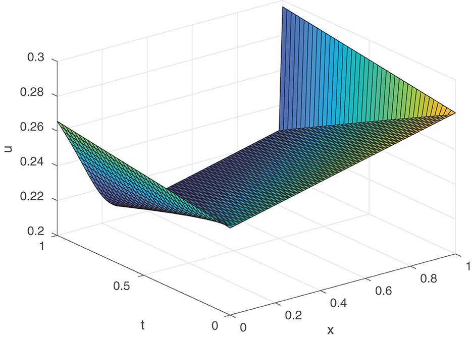
Figure 1. Numerical solutions of Example 4.1 using the proposed method for T = 1, M = 64, N = 40 and ε = 10⁻⁴. A layer is observed near x = 1.

Since the exact solution of this problem is not known, for each ε, the maximum pointwise error is calculated using double mesh principle [18] given by

$E_{\epsilon }^{M,N}={\displaystyle \underset{(x_m,t_n)\in D^{M,N}}{max}}|u_{m;M}^{n;N}-u_{2m;2M}^{2n;2N}|,$

where $u_{m;M}^{n;N}$ and $u_{2m;2M}^{2n;2N}$ are approximate solutions to problem (3.9) on D^{M, N} and D^{2M, 2N}, respectively. The corresponding order of convergence is given by

$R_{\epsilon }^{M,N}={log}_2\left(\frac{E_{\epsilon }^{M,N}}{E_{\epsilon }^{2M,2N}}\right).$

In Tables 1, 2, we compute the maximum absolute errors and the corresponding order of convergences using the proposed method for α = β = 1, γ = 0.5 and various values of ε with fixed values of M and N, respectively. From these results, we can observe that the method is ε-uniform convergent of order one both in time and space. This confirms the theoretical error results.

TABLE 1

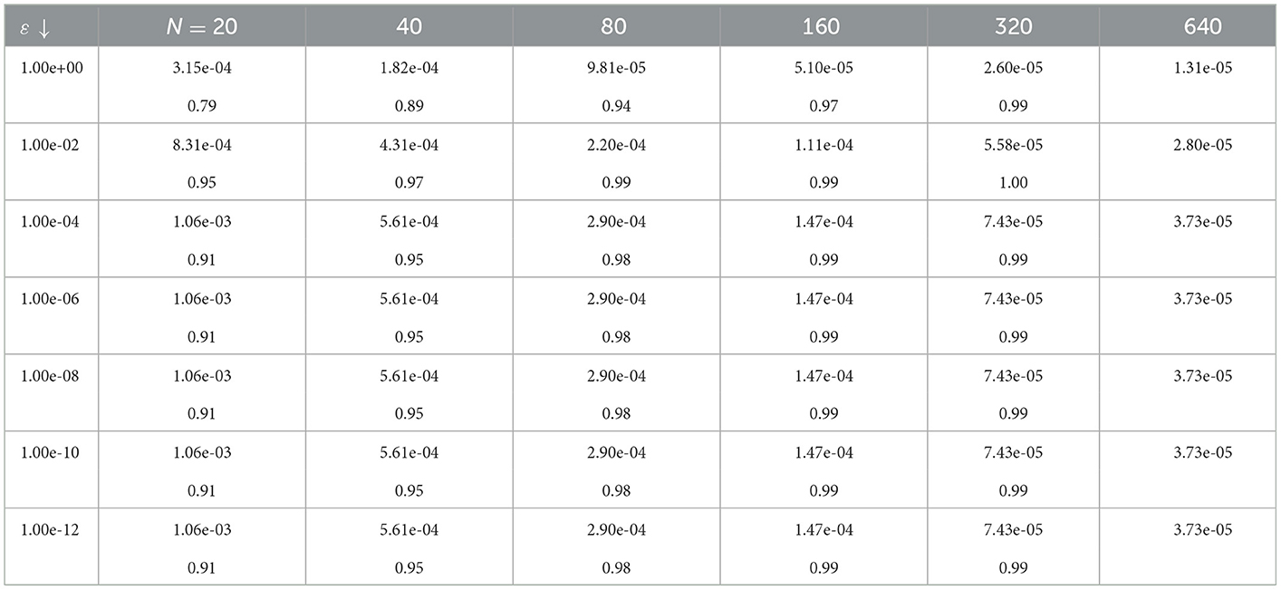
Table 1. Maximum absolute errors for Example 4.1 for M = 32 at the number of intervals N.

TABLE 2

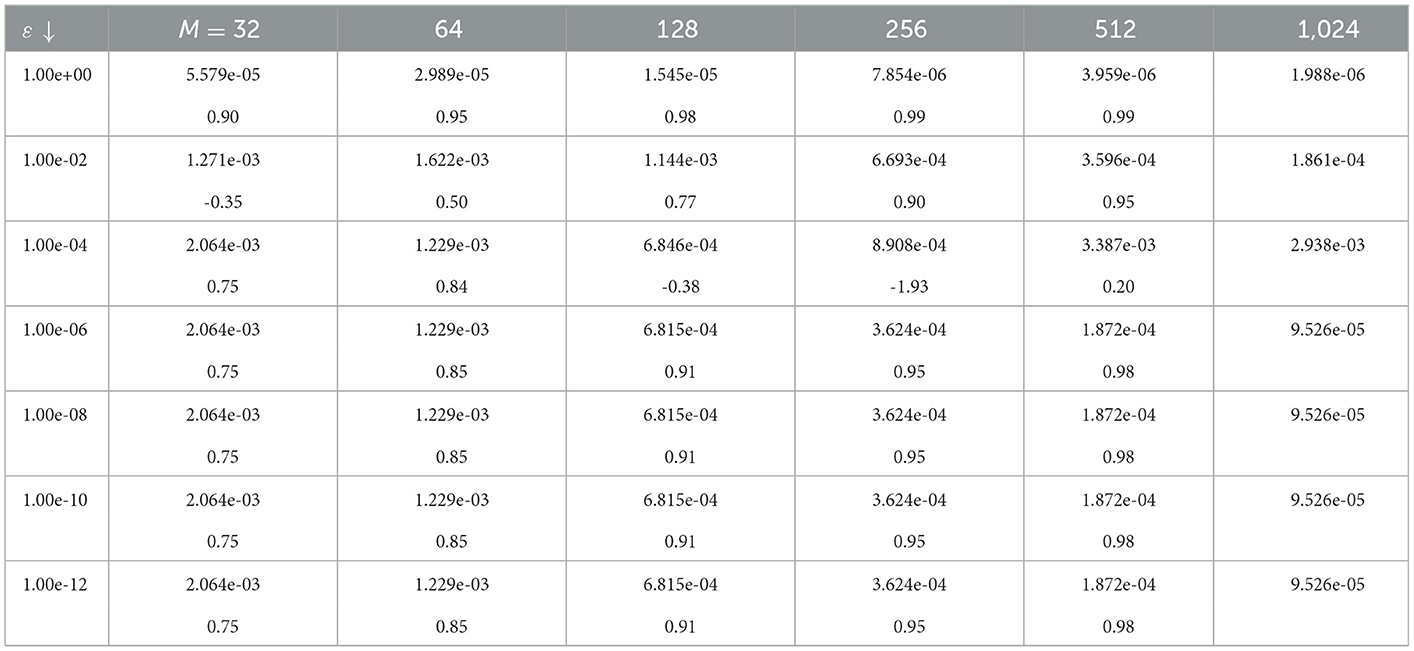
Table 2. Maximum absolute errors for Example 4.1 for N = 10 at the number of intervals M.

Table 3 compares absolute errors at some values of x and t using the proposed method and methods in [7, 19] and the nonlinear nonstandard finite difference (NNSFD) method given by

$\begin{array}{l}\frac{u_m^{n+1}-u_m^n}{\varphi (\Delta t,\epsilon )}-\epsilon \frac{u_{m+1}^{n+1}-2u_m^{n+1}+u_{m-1}^{n+1}}{{({\psi }_m^{n+1})}^2(h,\epsilon )}+a_m^{n+1}\frac{u_m^{n+1}-u_{m-1}^{n+1}}{h}\\ +b_m^{n+1}{u}_m^{n+1}=0,& (4.1)\end{array}$

where the denominator functions

$\varphi \left(\Delta t,\epsilon \right)=\frac{e^{\epsilon \Delta t}-1}{\epsilon },{\left({\psi }_m^{n+1}\right)}^2\left(h,\epsilon \right)=\frac{h\epsilon }{a_m^{n+1}}\left(\text{exp}(\frac{a_m^{n+1}h}{\epsilon })-1\right).$

The nonlinear system (4.1) can be easily solved using Newton's method (see in [7]). The solution at the previous time-step is taken as the initial estimate. The methods considered in [7] and [19] are NSFD methods and variational iteration method (VIM), respectively. From the table, we observe that our proposed method gives more accurate results.

TABLE 3

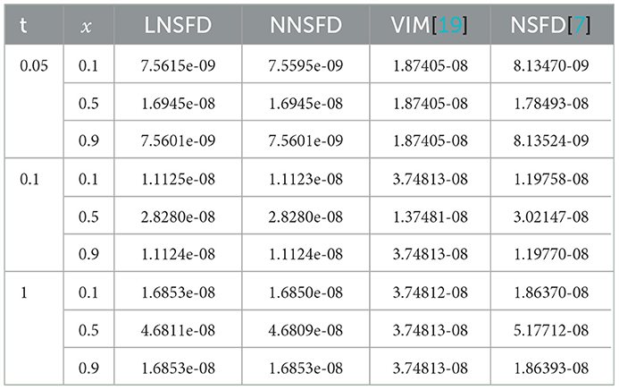
Table 3. Comparison of absolute errors for Example 4.1 using the proposed scheme (LNSFD) with results of [7, 19] and NNSFD for ε = 1, α = β = 1, γ = 0.001 at some values of x and t.

Also, in Table 4, we compare the CPU times required to compute the solutions of Example 4.1 for M = 10, N = 2000, α = β = 1, γ = 0.001, T = 10 using the LNSFD and NNSFD methods. As one can observe in the table, the CPU time for NNSFD is larger than the LNSFD.

TABLE 4

Table 4. CPU time for Example 4.1.

Example 4.2. Consider the following SPBHE [2]:

$\begin{array}{l}\{\begin{array}{l}\frac{\partial u}{\partial t}-\epsilon \frac{{\partial }^{2}u}{\partial x^2}+u\frac{\partial u}{\partial x}-(1-u)(u-0.5)u=0,(x,t)\in (0,1)\times (0,1],\\ u(x,0)=1+sin(\pi x/2),0<x<1,\\ u(0,t)=1,u(1,t)=2,0\le t\le 1.\end{array}\end{array}$

5. Conclusion

In this paper, a nonstandard finite difference method for a singularly perturbed Burgers-Huxley equation has been developed. First, the backward-Euler scheme was applied to discretize the problem (1.1) with respect to time derivative and the upwind nonstandard finite difference scheme on uniform mesh to approximate the spatial derivative. Then, the presented method was proved to be first-order convergent in both the spatial and temporal variables. Numerical results are given in Figures 1, 2 and in Tables 1–6 for two test examples to confirm the theoretical results and to compare with recent results. It has been observed from these figures and tables that the numerical results are in agreement with the theoretical findings. For ε = 1, in Table 3, comparisons with the NNSFD and the VIM of [19] and the NSFD method of [7] reveal that the proposed NSFD method gives more accurate results. In addition, the present method is also applicable when 0 < ε < 1. Thus, in all cases, the present method produces more accurate results than the existing schemes.

FIGURE 2

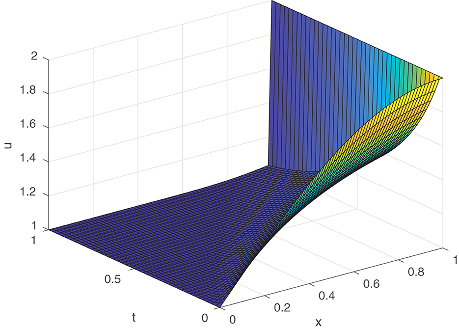
Figure 2. Numerical solutions of Example 4.2 using the proposed method for T = 1, M = 64, N = 40 and ε = 10⁻⁴. A layer is observed near x = 1.

TABLE 5

Table 5. Maximum absolute errors for Example 4.2 for M = 32 at the number of intervals N.

TABLE 6

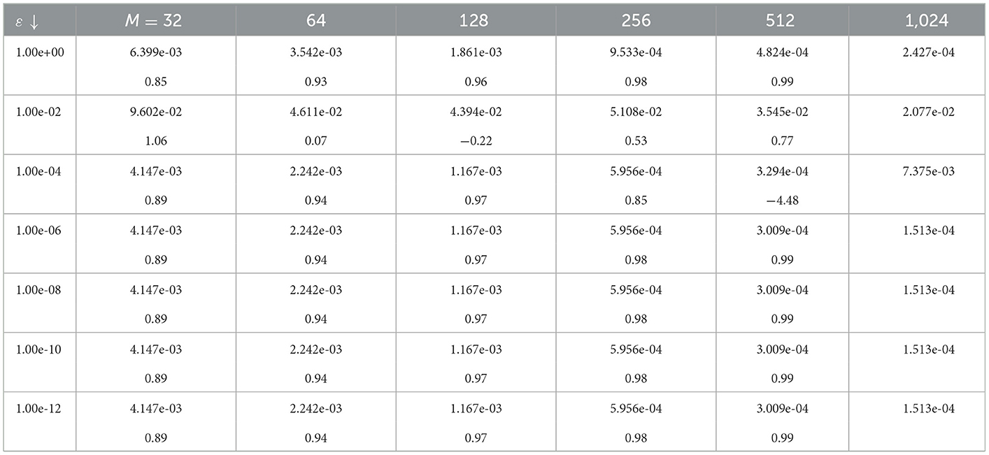
Table 6. Maximum absolute errors for Example 4.2 for N = 10 at the number of intervals M.

For future work, one may proceed with a higher order scheme for the problem under consideration for example by using the Crank-Nicolson method or those presented in [20, 21]. We are currently working in this direction. Also to note is that higher order parameter-uniform numerical methods for Burgers-Huxley equations are quasi-absent. The design of direct higher order parameter-uniform convergent methods is thus an interesting direction to explore.

Data availability statement

The original contributions presented in the study are included in the article/supplementary material, further inquiries can be directed to the corresponding author.

Author contributions

ED constructed the scheme and implemented the MATLAB code under JM's supervision. All authors participated in the analysis of the theoretical results and in the writing of the manuscript.

Acknowledgments

ED acknowledges the support received from the Department of Applied Mathematics of the Adama Science and Technology University which ensured that the author is registered for his Ph.D. study at the University for 4 years.

Conflict of interest

The authors declare that the research was conducted in the absence of any commercial or financial relationships that could be construed as a potential conflict of interest.

Publisher's note

All claims expressed in this article are solely those of the authors and do not necessarily represent those of their affiliated organizations, or those of the publisher, the editors and the reviewers. Any product that may be evaluated in this article, or claim that may be made by its manufacturer, is not guaranteed or endorsed by the publisher.

References

1. Kaushik A, Sharma MD. A uniformly convergent numerical method on non-uniform mesh for singularly perturbed unsteady Burger-Huxley equation. Appl Math Comput. (2008) 195:688–706. doi: 10.1016/j.amc.2007.05.067

PubMed Abstract | CrossRef Full Text | Google Scholar

2. Liu LB, Liang Y, Zhang J, Bao X. A robust adaptive grid method for singularly perturbed Burger-Huxley equations. Elect Res Arch. (2020) 28:1439. doi: 10.3934/era.2020076

CrossRef Full Text | Google Scholar

3. Kadalbajoo MK, Sharma KK, Awasthi A. A parameter-uniform implicit difference scheme for solving time-dependent Burgers' equations. Appl Math Comput. (2005) 170:1365–93. doi: 10.1016/j.amc.2005.01.032

CrossRef Full Text | Google Scholar

4. Wang X, Zhu Z, Lu Y. Solitary wave solutions of the generalised Burgers-Huxley equation. J Phys A Math Gen. (1990) 23:271. doi: 10.1088/0305-4470/23/3/011

CrossRef Full Text | Google Scholar

5. Wazwaz AM. Travelling wave solutions of generalized forms of Burgers, Burgers-KdV and Burgers-Huxley equations. Appl Math Comput. (2005) 169:639–56. doi: 10.1016/j.amc.2004.09.081

CrossRef Full Text | Google Scholar

6. Yefimova OY, Kudryashov N. Exact solutions of the Burgers-Huxley equation. Appl Math Mech. (2004) 3:413–20. doi: 10.1016/S0021-8928(04)00055-3

CrossRef Full Text | Google Scholar

7. Appadu AR, Inan B, Tijani YO. Comparative study of some numerical methods for the Burgers-Huxley equation. Symmetry. (2019) 11:1333. doi: 10.3390/sym11111333

CrossRef Full Text | Google Scholar

8. Derzie EB, Munyakazi JB, Dinka TG. Parameter-uniform fitted operator method for singularly perturbed Burgers-Huxley equation. J Math Model. (2022) 10:515–34. doi: 10.22124/jmm.2022.21484.1883

CrossRef Full Text | Google Scholar

9. Gupta V, Kadalbajoo MK. A singular perturbation approach to solve Burgers-Huxley equation via monotone finite difference scheme on layer-adaptive mesh. Commun Nonlinear Sci Numer. (2011) 16:1825–44. doi: 10.1016/j.cnsns.2010.07.020

CrossRef Full Text | Google Scholar

10. Mickens RE. Nonstandard finite difference models of differential equations. World Scientific. (1994). doi: 10.1142/2081

CrossRef Full Text | Google Scholar

11. Anguelov R, Lubuma JMS. Contributions to the mathematics of the nonstandard finite difference method and applications. Numer Methods Partial Differ Equ. (2001) 17:518–43. doi: 10.1002/num.1025

CrossRef Full Text | Google Scholar

12. Kadalbajoo MK, Gupta V. Hybrid finite difference methods for solving modified Burgers and Burgers-Huxley equations. Neural Parallel Sci Comput. (2010) 18:409–22.

Google Scholar

13. Mickens RE. Advances in the applications of nonstandard finite difference schemes. World Scientific. (2005). doi: 10.1142/5884

CrossRef Full Text | Google Scholar

14. Mickens RE. Calculation of denominator functions for nonstandard finite difference schemes for differential equations satisfying a positivity condition. Numer Methods Partial Differ Equ. (2007) 23:672–91. doi: 10.1002/num.20198

CrossRef Full Text | Google Scholar

15. Kumari A, Kukreja V. Robust septic Hermite collocation technique for singularly perturbed generalized Hodgkin-Huxley equation. Int J Comput Math. (2022) 95:24. doi: 10.1080/00207160.2021.1939317

CrossRef Full Text | Google Scholar

16. Kumari A, Kukreja V. Error bounds for septic Hermite interpolation and its implementation to study modified Burgers' equation. Numer Algorithms. (2022) 89:22. doi: 10.1007/s11075-021-01173-y

CrossRef Full Text | Google Scholar

17. Munyakazi JB, Patidar KC. Limitations of Richardson's extrapolation for a high order fitted mesh method for self-adjoint singularly perturbed problems. J Appl Math Comput. (2010) 32:219–36. doi: 10.1007/s12190-009-0245-6

CrossRef Full Text | Google Scholar

18. Doolan EP, Miller JJ, Schilders WH. Uniform Numerical Methods for Problems with Initial and Boundary Layers. Dublin: Boole Press. (1980).

Google Scholar

19. Batiha B, Noorani M, Hashim I. Application of variational iteration method to the generalized Burgers-Huxley equation. Chaos, Solitons & Fractals. (2008) 36:660–3. doi: 10.1016/j.chaos.2006.06.080

CrossRef Full Text | Google Scholar

20. Kovacs E, A. class of new stable, explicit methods to solve the non-stationary heat equation. Numer Methods Partial Differential Eq. (2021) 37:2469–89. doi: 10.1002/num.22730

CrossRef Full Text | Google Scholar

21. Nagy A, Saleh M, Omle I, Humam K, Kovacs E. New stable, explicit, shifted-hopscotch algorithms for the heat equation. Math Comput Appl. (2021) 26:61. doi: 10.3390/mca26030061

PubMed Abstract | CrossRef Full Text | Google Scholar