Magnetic resonance imaging enhancement using prior knowledge and a denoising scheme that combines total variation and histogram matching techniques

Introduction: Brain perfusion-weighted images obtained through dynamic contrast studies play a critical and clinical role in diagnosis and treatment decisions. However, due to the patient's limited exposure to radiation, computed magnetic resonance imaging (MRI) suffers from low contrast-to-noise ratios (CNRs). Denoising MRI images is a critical task in many e-health applications for disease detection. The challenge in this research field is to define novel algorithms and strategies capable of improving accuracy and performance in terms of image vision quality and computational cost to process data. Using MRI statistical information, the authors present a method for improving image quality by combining a total variation-based denoising algorithm with histogram matching (HM) techniques.

Methods: The total variation is the Rudin–Osher–Fatemi total variation (TV-ROF) minimization approach, TV-L2, using the isotropic TV setting for the bounded variation (BV) component. The dual-stage approach is tested against two implementations of the TV-L2: the split Bregman (SB) algorithm and a fixed-point (FP) iterations scheme. In terms of HM, the study explores approximate matching and the exact histogram matching from Coltuc.

Results: As measured by the structural similarity index (SIMM), the results indicate that in the more realistic study scenarios, the FP with an HM pairing is one of the best options, with an improvement of up to 12.2% over the one without an HM.

Discussion: The findings can be used to evaluate and investigate more advanced machine learning-based approaches for developing novel denoising algorithms that infer information from ad hoc MRI histograms. The proposed methods are adapted to medical image denoising since they account for the preference of the medical expert: a single parameter can be used to balance the preservation of (expert-dependent) relevant details against the degree of noise reduction.

1. Introduction

The introduction of computed tomography (CT) and, later, magnetic resonance imaging (MRI) in the 1980s resulted in a plethora of applications of these imaging methods to head and neck oncology. MR imaging is a rapidly evolving field that is replacing CT in the majority of extracranial head and neck lesions: tumors of the skull base, paranasal sinuses, nasopharynx, parapharyngeal space, and oral cavity, pharynx, and larynx carcinomas. Because of its superior sensitivity in detecting small lesions and superior accuracy in staging the lesion and narrowing the diagnostic possibilities, MR imaging is the method of choice for the detection and staging of skull base lesions. MRI more precisely shows the extent of a tumor in the paranasal sinuses, and multiplanar imaging outlines intracranial extension. MR imaging is more accurate than CT in differentiating parapharyngeal lesions and can more accurately detail the extent of tumor tissue in squamous cell carcinoma of the oral cavity, pharynx, and larynx. It is more sensitive than CT in detecting tumor tissue invasion into the mandible or laryngeal cartilage. Brain perfusion-weighted images obtained through dynamic contrast studies play a critical clinical role in diagnosis and treatment decisions. However, because of the patient's limited exposure to radiation, computed MRI images have a low contrast-to-noise ratio (CNR). Moreover, quantitative imaging is becoming increasingly common as radiological technology progresses. Quantitative imaging will change how we approach to care in the age of customized medicine, like the use of quantitative hepatic MRI involving fat and iron deposition [1].

Radiogenomics can help diagnose, prognosis, and treat cancer; at the same time, imaging phenotypes and multi-omic biological data may lead to new cancer prognostic models, patient treatment strategies, and survival predictors [2]. Diagnostic imaging has grown technologically and commercially, and large amounts of data do not always allow for their full exploitation. Moreover, digital platforms and applications like big data are needed to manage diagnostic images correctly [3]. Furthermore, there are many unexplored potentials of the Digital Imaging and COmmunications in Medicine (DICOM) standard for leveraging the radiological workflow from a big data perspective [4].

Because medical imaging is critical in assessing a patient's health and providing appropriate treatment, the presence of numerous overlapped items in the image complicates the diagnostic procedure. Medical images do not provide enough information to diagnose accurately due to low lighting settings, environmental sounds, technical limitations of imaging instruments, and other factors. For example, a high-contrast image can also reveal a region of interest (ROI) or an object. Numerous contrast and quality enhancement approaches for medical images have been proposed; for example, histogram equalization, gamma correction, and transform-based techniques are used to improve medical images, while denoising can aid in image cleaning. However, image histograms cannot encode spatial image variation [5]. Noise and distortions are frequently present in medical images. Some texture-based features that should indicate tissue structure may actually reflect the scanner's uneven sensitivity. The impact of various normalization approaches and the number of intensity levels on texture categorization is still being investigated [6].

In many e-health applications for disease detection, denoising MRI images is a critical task. Indeed, noise during image collection hinders both human and computer interpretation [7]. In this research field, the challenge is to define novel algorithms and strategies capable of improving accuracy and performance in terms of image vision quality and computational cost to process data. The denoising scenario is a significant research topic in the development and implementation of algorithms capable of removing artifacts from images. Bazin et al. [8] presented a denoising strategy for multi-parametric quantitative MRI that combines local PCA with a reconstruction of the complex-valued MR signal to define stable noise estimates, while Ouahabi [9] showed that wavelet denoising algorithms reduced noise.

Inferring correct information from digital images acquired by some devices requires multiple reconstruction methods to reduce artifacts, sampling errors, and noise. In many research areas, such as geophysics, e-health monitoring, and biomedical imaging, solving an image processing problem (denoising, filtering, restoration, segmentation, etc.) is a crucial computational task (see, for example, Benfenati and Ruggiero [10, 11], Hammernik et al. [12], Lanza et al. [13], Morigi et al. [14], De Asmundis et al. [15], and Zanetti et al. [16]).

This research problem is typically defined as an inverse problem in mathematical modeling, and it is typically a heavy computational task that necessitates the use of high-performance computing (HPC) environments (see Lustig and Martonosi [17] and Quan et al. [18]). Many noise-removal techniques have been discussed and developed over the last decade while avoiding excessive blurring for small structures in MRI images. Unfortunately, most strategies do not take into account morphological a priori information embedded in an MRI image I; this type of image differs significantly from a general grayscale image. The intensity distribution of MRI images follows a suitable model that describes the target's anatomy (e.g., a human brain). In Luo et al. [19], the authors propose an expectation-maximization (EM) adaptation that uses a generic prior learned from a generic external database and adapted it to the noisy images; the proposed algorithm is based on a Bayesian hyper-prior perspective. The experimental results show that the proposed adaptation algorithm consistently outperforms the control algorithm in terms of denoising. They focus on the maximum a posteriori (MAP) approach, a Bayesian approach that tackles image denoising by maximizing the posterior probability, but MAP optimization is critically dependent on the modeling capability of the prior, and seeking the prior for the entire image is practically impossible due to its high dimensionality.

This article proposes a method for improving image quality after applying a smart denoising algorithm that relies on a priori information on MRI data, which can be stored in a dictionary. The obtained results can be used to analyze and study more complex approaches based on machine learning methodologies in order to design novel denoising algorithms that infer knowledge from ad hoc MRI look-up table dictionaries. We investigated how to denoise MRI images using application domain priors. This study has two goals: it proposes a model for image entrenchment and restoration using a novel two-stage process, and it provides insights for future models.

Our fundamental idea is to employ a priori information from a pre-selected target to improve the restored image quality after applying a denoising method. In this case, a two-stage technique is appropriate, which is summarized as follows:

a) applying a suitable image denoising scheme to compute J from a noisy image I and

b) improving the quality of J by means of a dictionary containing a priori information on MRI images (the target).

Step a), i.e., image denoising, is an inverse problem, and it is well known that regularization techniques have to be considered to solve it. Given an input noisy image I of dimension N×M, solution J of the image denoising task is obtained by solving the following regularized optimization problem:

$\begin{array}{ll}{u}^{*}:={\displaystyle \underset{u}{argmin}}\left|\text{Ψ}(u)\right|+H(u,f),& (1)\end{array}$

where | · | is a norm and the convex functions Ψ(u) and H(u, f) are called the regularization and the fidelity term respectively. In practice, u generally denotes the column vector u ∈ ℝ^{N × M} by the lexicographical ordering of a two-dimensional MRI, u^* ∈ ℝ^{N × M} is a vector that represents the desired image, and f represents the noisy image. More in detail, this study deals with the accurate numerical solution of an inverse image processing problem by combining classical denoising strategies with post-processing techniques where the target is an intensity distribution of the value of u^* that is close to the image histogram.

In step b), we assume that the MRI image J has L different levels of pixel intensity; a histogram of B disjoint bins is defined as a discrete function h(b_i) = n_i, where b_i is the ith bin and n_i is the number of pixels in the image belonging to the such bin. Commonly L = B, and for an 8-bit image L = 256 and it is possible to normalize the histogram in order to have an estimate of the probability at which each level can occur. This is done by calculating

$p(b_i)=\frac{n_i}{N},\text{\hspace{1em}\hspace{1em}where }N={\displaystyle \sum _i{n}_i},$

as one would expect, $\sum _{i}p(b_i)=1$. The importance of investigating histograms is underlined by several authors. The analysis of histograms in medical images can provide two benefits: first, to improve diagnosis like in Schob et al. [20] where valuable information on tumors can be provided through histogram analysis; the second, which has to be done before any analysis, is to improve the quality of the image like in Senthilkumaran and Thimmiaraja [21] where simple histogram equalization is applied to enhance MRI brain images. Moreover, histograms are equivalent to intensity mapping functions [22, 23]. Finally, some numerical experiments show that using a priori information on MRI data can improve image quality after applying a smart denoising algorithm [7, 24–26].

At this point, we should recall that an image can be defined as a two-dimensional function u(r, c), where r and c are plane coordinates for the row and column of the 2D image. The amplitude of u at any pair of coordinates (r, c) is called the image's intensity or gray level at that point. Digital images have discrete quantities of r, c, and u. The image source determines the physical meaning of u's amplitude [23]. When an image is created physically, its intensities are proportional to the energy radiated by a physical source, such as electromagnetic waves, so u is nonzero and finite and typically, values for u are scaled in the range [0, 1]. For a digital image, we should convert the continuous sensed data into the finite set {0, 1, .., 255}. A digital grayscale image can thus be described as a map of the type u:I → [0, 255] ⊂ ℕ and consequently have a codomain of cardinality 256, where the cardinality of a set refers to the number of elements it is composed of.

The suggested method can be ideal for medical denoising because it considers a single parameter that can balance the preservation of (expert-dependent) significant features against noise reduction. One of the major issues that we will address is that, while we assume u ∈ ℝ^N×M for denoising, the cardinality of the codomain u is usually L = 256 for typical images, but it is larger for MRI.

The article is organized as follows: Section 2 is devoted to an overview of the denoising models and the construction of a target by using histogram information. Section 2 also includes the strategy for combining denoising algorithms and histogram matching. Section 3 is concerned with numerical experiments and their outcomes. Finally, the study is completed in Section 4.

2. Materials and methods

This section provides an overview of denoising models and the construction of a target using histogram data. The strategy for combining denoising algorithms and histogram matching is then finally addressed.

Assume we have an image I of size N×M with values in the range [0, 1]. The cleaned image is called J. Each image can have several values, i.e., depending on the cardinality of the codomain, all possible levels are divided into L levels; in the case of a b-bit image, we have L = 2^b.

2.1. Denoising algorithms

A typical approach to the denoising problem is based on the idea that an image f may be divided into two parts: a structural component (the objects in the image) and a textural part (the fine details plus the noise) [27]. Total variation denoising (TVD) is based on the idea that images with excessive and possibly spurious detail have high TV. According to this principle, TV denoising tries to find an image with less TV while being similar to the input image, which is controlled by the regularization parameter. Denoising tends to produce cartoon-like images, or piecewise-constant images [28].

This is known as the ROF method (from the initials of the authors' surnames, Rudolf, Osher, and Fatemi) and was first presented in Rudin et al. [29], also known as TV-L². This approach divides the input image, f, into two components: a structure component u ∈ BV (bounded variation) and a texture component u−f in L².

In this general formulation, the bounded variation seminorm is defined as follows:

$\begin{array}{r}\Vert u{\Vert }_{BV(I)}:={\displaystyle {\int }_I\Vert Du(}x)\Vert dx:=\\ \sup \left\{{\displaystyle {\int }_{I}u}\nabla ·p\text{ s.t. }p:I\to {ℝ}^2,p\in C^1(I),\Vert p\Vert \le 1,\forall x\in I\right\}\end{array}$

on the unit square I = [0, 1]² where D = [D_x; D_y] is the gradient operator ∇ in the discrete setting, and D_x, D_y denote the horizontal and vertical partial derivative operators, respectively [30]. Since TV-ROF uses the ℓ1-norm for the BV, the optimization problem (1) becomes a ℓ1-regularization problem.

By minimizing (Equation 1) defined as follows:

$\begin{array}{ll}{u}^{*}:=\underset{u}{\arg \min }\Vert u{\Vert }_{BV}+\frac{\mu }{2}\Vert u-f{\Vert }_2^2,& (2)\end{array}$

in which an image u^* is recovered starting from its noisy version f, and where Du≈∇u is the gradient of u, and the term μ denotes a regularization parameter that balances the relative weights of the fidelity and the regularization terms.

As the authors in Rudin et al. [29] point out, the use of L², for the texture component, makes this algorithm a kind of universal decomposer, capable of removing most types of existing noise. It performs particularly well on textures with oscillatory patterns. Alliney [31] and Nikolova [32] proposed replacing the L² norm of the ROF model with the L¹ norm. Nikolova demonstrated in one of her works [32] that looking for the part texture of an image within a space like L¹ is a procedure particularly suitable for removing salt and pepper noise. When researchers focused on compressed sensing, which allows images and signals to be reconstructed from small amounts of data, L¹-regularized optimization problems were investigated, and Goldstein and Osher [33] proposed a split Bregman approach to address L¹-regularized problems.

Because it is difficult to accurately describe the gradient for discrete images using finite differences, the regularization term in Equation 2, which is defined in the BV space, can be numerically approximated in a variety of ways with the most well-known approaches being the isotropic or anisotropic TV setting. The traditional, so-called “isotropic” definition of discrete TV is far from isotropic, but it works reasonably well in practice [34]. The TV-ROF is isotropic or rotation-invariant, but quantifying the isotropy of a TV functional is difficult because ℤ² is not isotropic, and there is no unique way to define image rotation. However, after a 90-degree rotation or a horizontal or vertical flip, the image's TV should remain unchanged [34]. On the other hand, the term anisotropic is used because this variation divides vertical and horizontal components in the same way that anisotropic diffusion does. As a result, it lacks the rotational invariant term seen in the Isotropic approach [35]. More in detail, we have

$\Vert u{\Vert }_{BV;iso}=\Vert Du{\Vert }_{2,1}={\Vert \sqrt{\left|D_{x}u\right|+|D_{y}u}|\Vert }_1$

for the isotropic setting, and

$\Vert u{\Vert }_{BV;ani}\text{=}\Vert Du{\Vert }_1=\Vert D_{x}u{\Vert }_1+\Vert D_{y}u{\Vert }_1$

for the anisotropic one [36]. Note that we will write more compactly d_x: = D_xu and d_y: = D_yu. The distinction between the anisotropic and isotropic problems is in how we calculate d_x and d_y. In contrast to the anisotropic problem, d_x and d_y are coupled together in the isotropic problem.

A comprehensive theoretical analysis of the ROF model has been discussed by Chambolle and Lions [37]. The following are some of the nice features of this problem that have been explored in the literature: (i) TV-ROF deals properly with edges and noise removal in grayscale images; (ii) the TV term discourages the solution from having oscillations; (iii) the second term encourages the solution to be close to the observed image u^*. Unfortunately, the model has several drawbacks, and it has a number of flaws, in particular, the model causes a loss of contrast and the staircase effect, i.e., pixelization of the image at smooth regions and loss of finely textured regions. Finally, bad decomposition of the image u^* in cartoon and texture (noise) is a general open issue [38].

In order to overcome these difficulties, several strategies have been proposed (see Benfenati and Ruggiero [11] and Setzer et al. [39]). The most commonly used approach consists in modifying the cost function by adding penalty terms R(u) in Equation (2), thus defining the new model:

$\begin{array}{ll}{u}^{*}:=\underset{u}{\arg \min }\Vert u{\Vert }_{BV}+\frac{\mu }{2}\Vert u-f{\Vert }_2^2+R(u).& (3)\end{array}$

the choice of R(u) depends on the kind of a priori information available on the problem to be solved. In this article, our approach is quite different, and it consists of solving the original denoising problem (Equation 2) and after considering post-processing techniques to improve the denoising task as reported in the next sections.

We concentrate on total variation because the variation regularization problem is cutting-edge in the noise removal process. The main hypothesis underlying this algorithm is that images with excessive and possibly spurious detail have a high total variation. In other words, the integral of the absolute gradient of the data is large. Under these conditions, minimizing a functional with the fidelity term and the total variation of the image is useful for removing unwanted detail while preserving critical information such as edge.

In terms of other more appropriate penalty terms to be used in equation (3). The TV noise-removal method outperforms simple strategies such as linear smoothing or median filtering, which reduce noise while smoothing away edges to varying degrees. Total variation denoising, on the other hand, is a remarkably effective edge-preserving approach, preserving edges while smoothing away noise in flat regions even at low signal-to-noise ratios. We propose in this article to add more penalty H(u) that is related to some statistical hypothesis on the pixel distribution. This strategy allows us to embed certain image contrast information directly into the mathematical model, and to the best of our knowledge, only the penalty term is capable of preserving this information.

There are several schemes used in the literature to solve the TV-ROF problem (2) and its variants. This research examines two denoising strategies: (i) the split Bregman algorithm (SBA), proposed in Goldstein and Osher [33]; (ii) the fixed-point (FP) iterations [40].

Our decision to discuss two algorithms is to demonstrate how these two methods can solve the problem and, eventually, how they can be modified by including our penalty term suggestion. Since the solution is unique, the two different algorithms converge to the same solution but in two distinct ways. Furthermore, they will always make a numerical error and approximate the unique solution with a certain tolerance. This is why we set the same tolerance for both methods. Furthermore, depending on the method, the same tolerance might be accomplished with a variable number of steps. In our dual-stage technique, we want to emphasize the overall number of steps necessary, which is the number of denoiser iterations plus one for histogram matching.

2.1.1. Split Bregman algorithm

The SBA is a special case of alternating direction method of multipliers (ADMMs) [41]. The SBA has been successfully used in solving several regularized optimization problems [42–44], and it has been shown to be especially effective for problems involving TV regularization [39, 45, 46].

In the isotropic TV model, we solve the following problem:

$u^{*}:=\underset{u}{\arg \min }\Vert Du{\Vert }_{2,1}+\frac{\mu }{2}\Vert u-f{\Vert }_2^2.$

This problem is rewritten as a constrained problem,

$\underset{u}{\arg \min }\Vert (d_x,d_y){\Vert }_{2,1}+\frac{\mu }{2}\Vert u-f{\Vert }_2^2,$

such that d_x = D_xu and d_y = D_yu and we relax the constraints and solve the unconstrained problem

$\underset{u,d_x,d_y}{\arg \min }\Vert (d_x,d_y){\Vert }_{2,1}+\frac{\mu }{2}\Vert u-f{\Vert }_2^2+\frac{\lambda }{2}\Vert d_x-u_x{\Vert }_2^2+\frac{\lambda }{2}\Vert d_y-u_y{\Vert }_2^2,$

where λ is the Lagrange multiplier, $u_x=D_x^{c}u$, $u_y=D_y^{c}u$ and D^c is the second order centered finite difference. Finally, by defining

$s^k=\sqrt{{\left|u_x^k+b_x^k\right|}^2+{\left|u_y^k+b_y^k\right|}^2},$

we consider the minimization of d_x and d_y, by approximating $||(d_x^k,d_y^k)||{}_{2,1}$ by s^k. Because we can now obtain the value of the derivative by minimizing, it is no longer necessary, for instance, for us to calculate a derivative for d_x, such as D_xu as in u_x.

In this section, we refer to the algorithm proposed in Goldstein and Osher [33]. The specific steps and indexes utilized are shown in Algorithm 1. Note that Isotropic TV denoising is our SBA implementation and is inspired by the study of Bush [47].

ALGORITHM 1

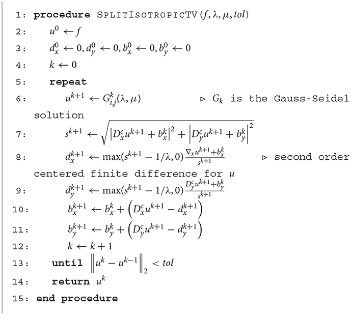
Algorithm 1. Implemented split Bregman isotropic TV denoising.

We note that the value λ ≥ 0 is a Lagrange multiplier and G is the Gauss–Seidel function written componentwise as follows:

$\begin{array}{r}{G}_{ij}^k=\frac{\lambda }{\mu +4\lambda }(u_{i+1,j}^k+u_{i-1,j}^k+u_{i,j+1}^k+u_{i,j-1}^k+\\ d_x{}_{i-1,j}^k-d_x{}_{i,j}^k+\mathrm{...}+\mathrm{...}\\ d_y{}_{i,j-1}^k-d_y{}_{i,j}^k-b_x{}_{i-1,j}^k+\\ b_x{}_{i,j}^k-b_y{}_{i,j-1}^k+b_y{}_{i,j}^k)+\\ \frac{\mu }{\mu +4\lambda }{f}_{i,j}.\end{array}$

2.1.2. Fixed-point iterations scheme

The second scheme we used to solve the optimization problem is based on what the authors in Vogel and Oman [40] call lagged diffusivity fixed point iteration, abbreviated by FP. This is done by considering the associated Euler–Lagrange equations of TV-ROF equation that are as follows:

$g(u):=(f-u)-\theta L_u(F)=0,$

where L_u is the diffusion operator whose action on a function p is given by :

$L_u(p):=-\nabla u·\left(\frac{1}{\sqrt{|\nabla u{|}^2+{\beta }^2}}\nabla p\right),$

and β is a positive parameter to correct the non-differentiability in zero, and θ is the regularization parameter. The formula for FP iteration is then (1 − θL(u^(k)))u^(k+1) = z, for k = 0, 1, …, so to obtain the new iterate u^(k+1), we solve a linear diffusion equation whose diffusivity depends on the previous iterate u^(k). The implemented algorithm is reported in Algorithm 2, where we have u^k = f − θ∇ ·p^k−1, and

$p^k=\frac{p^{k-1}-\alpha ·\nabla u^k}{(1+\alpha /g)·|\nabla u^k{|}^2},$

where $\alpha =\frac{1}{4\theta }$ and g = 1.

ALGORITHM 2

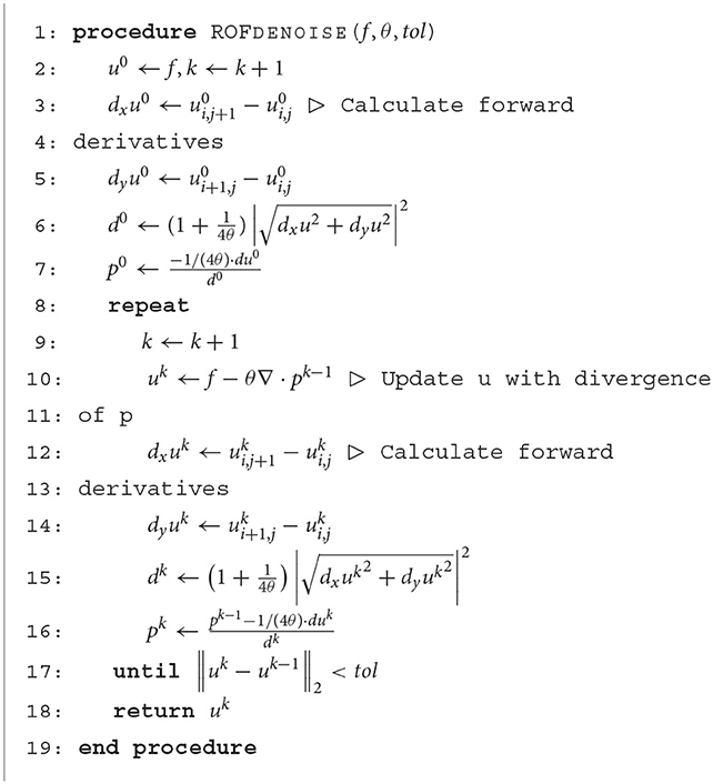
Algorithm 2. Implemented ROF denoising.

2.2. Construction of a target: The histogram approach

The histogram of a digital image with gray levels in the range [0, L − 1] shows how many times (frequency) each intensity value in an image occurs. As a result, a histogram for a grayscale image with intensity values in the range I(r, c) ∈ [0, L − 1] where r and c denote row and column, respectively, and they are utilized to identify each pixel of our image I, with the interval containing exactly L values [23]. For example, in an 8-bit grayscale image, L = 2⁸ = 256. Each histogram entry h(i) = n_i is described as the total number of pixels with intensity i for every 0 ≤ i ≤ L and $\sum _{i=0}^{L-1}{n}_i=n$. A normalized histogram is given by p(i) = n_i/n; this gives an estimate of the probability of occurrence of gray level i. Note that the sum of all components of a normalized histogram is equal to 1, i.e., $\sum _{i=0}^{L-1}p(i)=1$. In fact, histograms contain statistical data.

2.2.1. Histogram equalization

Histogram equalization is a technique for adjusting image intensities to enhance contrast. Many strategies for enhancing contrast have been explored in literature. Histogram equalization (HE) is one of the most extensively used techniques for improving low-contrast photos, as it keeps the histogram of light intensities of pixels within an image as consistent as possible. Calculating cumulative distributive function (CDF) is a common way to equalize the histogram of an image.

The histogram equalized image G, of a given image I, will be defined by

$G(r,c)=\lfloor (L-1){\displaystyle \sum _{n=0}^{I(r,c)}p}(n)\rfloor$

where ⌊a⌋ is the floor operator, which rounds down to the nearest integer that is less than or equal to a. This is comparable to changing the pixel intensities, i, of I by the function:

$T(i)=\lfloor (L-1){\displaystyle \sum _{n=0}^{i}p}(n)\rfloor .$

The motivation for this transformation comes from thinking of the intensities of I and G as continuous random variables X, V on [0, L − 1] with V defined by:

$V=T(x):=(L-1){\displaystyle {\int }_0^x{p}_X}(w)dw,$

where p_X and p_V are the probability density functions (PDFs) of I. T is the cumulative distributive function (CDF) of X multiplied by (L − 1). Assuming that T is differentiable and invertible, it can then be demonstrated that V defined by T(X) is uniformly distributed on [0, L − 1], namely $p_V=\frac{1}{L-1}$, where L is the number of levels greater than 2, i.e., when there are two levels we have a binary image [23].

The traditional HE algorithm has various flaws. For starters, when a histogram bin has a very large value, the transformation function has an extremely steep slope. Second, particularly for dark photos, HE changes from very low intensities to high intensities, which may increase noise components while lowering image quality. Third, because conventional HE is a fully automatic technique with no parameters, the level of contrast enhancement cannot be regulated.

Many strategies have been offered to alleviate these disadvantages, and histogram matching (HM) is one among them.

2.2.2. Histogram specification (or matching)

In general, HM is a technique that uses histogram information from an input image to compute the transformation function. As a result, HE can be thought of as a subset of HM.

In image analysis, the histograms corresponding to a pair of images are both required and sufficient for determining the intensity mapping function.

When we expect the histograms of scene radiance to remain roughly constant between images taken at different exposures, the intensity mapping function is determined by histogram specification. This means that in the presence of some scene, where registration would be difficult or impossible, the intensity mapping functions can be recovered [22].

One can transform a histogram into another one through histogram specification. Histogram specification (or matching) can be seen as a generalization of histogram equalization. The classical approach that formalizes histogram matching starts by considering the intensity as a continuous random variable (RV), with values in [0, L − 1], characterized by a probability density function (PDF). In this case, the formulation is straightforward.

Consider two RV, X₁ and X₂, and let F_X1 and F_X2 be the cumulative distribution function (CDF), respectively. The objective is to transform X₁ such that its PDF p_X1 becomes p_X2. The objective is to find a transformation T, such that x₂ = T(x₁). By noting that

$F_{{\text{X}}_1}(x)={\displaystyle {\int }_{-\infty }^x{p}_{{\text{X}}_1}}(w)dw,F_{{\text{X}}_2}(x)={\displaystyle {\int }_{-\infty }^x{p}_{{\text{X}}_2}}(w)dw.$

Using two transformation function T₁, T₂,

$v_1=T_1(x):=(L-1){\displaystyle {\int }_0^x{p}_{{\text{X}}_1}}(w)dw,$

$v_2=T_2(x)=(L-1){\displaystyle {\int }_0^x{p}_{{\text{X}}_2}}(w)dw$

creates two RV, V₁ and V₂, that are uniform. By imposing v₁ = v₂, the mapping T is $x_2=T(x_1)=T_2^{-1}(T_1(x_1))$, i.e., $T=T_1◦T_2^{-1}=F_{{\mathrm{\text{X}}}_1}◦F_{{\mathrm{\text{X}}}_2}^{-1}$.

Unfortunately, this process is dependent on strictly increasing functions, which are difficult to implement in a digital image. One possible method will be to use generalized inverse [48], as $T_1^{-}(x_2)=inf\left\{x\in ℝ:T_1(x)\ge x_2\right\}$. This produces a mapping between the two sets of bins in a discrete framework by obtaining an approximate matching.

In discrete histogram matching, it is difficult to rank (separate) equal intensity levels. Adding noise to the image can help distinguish between identical intensity levels. A different strategy is to differentiate each pixel of the image by ordering an N×M image pixels as I(r₁, c₁) ≺ I(r₂, c₂) ≺ ⋯ ≺ I(r_NM, c_NM), which results in an exact histogram matching [49].

Although the procedure just described is straightforward in principle, it is seldom possible in practice to obtain analytical expressions for T₁ and for $T_2^{-1}$. Fortunately, this problem is simplified considerably in the case of discrete values. The price we pay is the same as in histogram equalization, where only an approximation to the desired histogram is achievable. In spite of this, however, some very useful results can be obtained even with crude approximations.

Histogram matching (specification) is usually used to enhance an image when histogram equalization fails. Histogram matching can provide a processed image with the specified histogram, given the shape of the histogram that we desire in the enhanced image. After histogram matching, a source image resembles the target image in terms of histogram distribution when the histogram of a target image is specified. Histogram matching can be implemented with the following calculations, as shown in the following equations. For the source image, we can calculate the transformation as follows:

$\begin{array}{l}{s}_i=T_1(r_i)=(L-1)·{\displaystyle \sum _{j=0}^i}\frac{n_j}{n},i=0,1,2,\dots ,L-1,\end{array}$

where n is the total number of pixels in the image, n_j is the number of pixels that have gray level r_j, and L is the total number of possible gray levels in the image. Thus, an enhanced image is obtained by mapping each pixel with level r_i in the input image into a corresponding pixel with level s_i in the output image. Actually, this is the process of histogram equalization. Obviously, T₁(r_i) is an increasing monotonic function. Similarly, for the target image or the given group of categorized images, we have

$v_i=T_2\left(z_i\right).$

Considering v_i = s_i for histogram matching, the processed image is accordingly,

$\begin{array}{l}{z}_i=T_2^{-1}(v_i)=T_2^{-1}(s_i)=T_2^{-1}[T_1(r_i)],\\ i=0,1,2,\dots ,L-1.\end{array}$

A well-known method to map target images into categorized images comes from Coltuc et al. [49, 50] a family of moving average filters is designed starting with ϕ₁ having one-pixel size support and then, enlarging from the next ones while keeping the symmetry for a minimum increase of the filter support. The filter grows by considering squares increased or rotated at each step; this produces the ordering of image pixels.

Coltuc's approach has been improved by Nikolova et al. [51, 52] by using a variational approach. In the aforementioned study, Nikolova et al. minimized a functional of the form as follows

$J(u,f)=\text{Ψ}(u,f)+\beta \text{Φ}(u),$

where Ψ is the sum of a specific function ψ evaluated at the difference among u (function to minimize) and f (starting-original image) for each pixel and Φ is the sum for each pixel evaluated through a specific function ϕ evaluated in a vector of forward differences in horizontal and vertical directions.

The ordering problem is not important in exact histogram specification methods that are designed for real-valued data. In typical digital images, there are no true real values, and within many pixels, they must share a small range of values [52]. Another approach, like [53], instead of using functions, relaxes this property and use a one-to-many relation mapping.

Exact histogram matching solves a problem that is ignored by typical histogram modification approaches meant for real-valued data. Exact histogram specification methods for digital images have to deal with many pixels that have the same value. Because there are many ways to assign the prescribed values to the quantized values, digital image histogram specification is ill-posed [52]. The problem in the MRI case is that the granularity depends on various variables (acquisition methods, magnetization, noise, and discretization).

2.3. The MRI dual-stage denoising implementation

Here, we propose a two-stage TV denoising with histogram matching, where we try to mix the benefits of both approaches.

Our dual-stage procedure composes as follows:

1. Denoiser: a TV-ROF denoiser that iterates for a certain number of steps, until a relative error, less than Tol is achieved, by specifying its regularization parameter.

2. HM: a histogram matching technique that uses a specific histogram to match.

To validate the procedure, we used two different denoisers and HM. We tried two approaches for the denoiser:

• SB-ROF: the split Bregman isotropic TV Denoising, as described in Section 2.1.1.

• FP-ROF: the fixed-point iterations scheme, basically a simple ROF denoising algorithm described in Section 2.1.2.

The SB algorithm was used with λ = 4.95*10⁻² and μ = 1, while the FP algorithm with θ = (2/7)*10⁻¹.

In terms of the HM algorithm, we used two different functions in our tests:

Approx: the simplest histogram matching algorithm, which changes the input grayscale image so that the histogram of the output image closely matches the histogram of the reference image and

Exact: the exact histogram matching from Coltuc et al. [49, 50].

It is worth noting that in our implementation, the first function takes the target image as input, while the second takes the target histogram. In either case, we eventually settled on 8-bit images, i.e., histograms with L = 2⁸.

All of the results presented in this article were obtained on either a Windows system running Matlab^® R2022b or a Linux system running Matlab^® R2017b.

We used the Matlab^® function imhistmatch for the approximate approach. Instead of the default 64, the number of bins has been fixed at 265. The implementation assumes that values are real valued when processing the image histogram. The intensity value is represented by x and is assumed to be in the range [0, 1]. The histogram's L bins are each half-open intervals of width 1/(L − 1).

In such HM, we first compute the histogram of the reference image R, by generating vector and half-open intervals of width 1/(L − 1), and then adjust I using the reference histogram by computing the cumulative histogram and generating the transformation to intensity image. In fact, the function imhistmatch calls imhist first and then histeq. imhistmatch transforms a 2D image I and returns an output image J with a histogram that approximates the histogram of the reference image R. The number of bins b is usually 64; the higher the number, the higher the computational cost. The histogram is composed of b evenly spaced bins spanning the entire image data type. These bins also represent the maximum number of discrete data levels available. As b increases, the output histogram exhibits larger oscillations between nearby peaks. The histogram has L = 2^b bins for each half-open interval with width 1/(L − 1). The p-th bin, in particular, is the half-open interval:

$\frac{(p-1.5)}{(L-1)}\le x<\frac{(p-0.5)}{(L-1)},$

where x is the intensity value.

Finally, the exact HM is based on the work of Semechko [54]. The function takes as input a grayscale image I in 8 or 16 bits, as well as a specific histogram h with the length L, where L is the maximum number of pixel intensities. The number of histogram bins must correspond to the maximum number of gray levels in the image. We begin by assigning pixels in strict order using filters. We then adapt the provided histogram to meet the amount of image/foreground pixels by calculating the total number of image pixels and re-normalizing the histogram and frequency residuals, and finally redistributing residuals based on their magnitude. The histogram is then specified by converting it to raw intensity data. Finally, image pixels are rearranged according to pixel order, intensities are rearranged according to image position, and the image is reassembled.

We will see what happens to the image after we apply the histogram-matching technique in the results section.

2.4. MRI data model

This final subsection will discuss the data used in the experimental setup.

When discussing MRI scanners, we use the term Tesla (abbreviated by T) to refer to magnetic field strength; 3 Tesla is typical for MRI scanners (3T). 3T MRIs are used in clinical imaging; at the same time image noise is reduced, and scanning resolution is increased in new 7T MRI scanners for ultra-high resolution imaging. The size of each image pixel is referred to as spatial resolution, and more detailed, high-quality images result from higher MRI resolution.

The magnetic characteristics and amount of hydrogen nuclei in the observed area determine MR image contrast, and the repetition time (TR) and echo time (TE) are utilized to adjust image contrast. Several sequences with varying weightings can be used to select contrasts in the imaged area. Cerebrospinal fluid (CSF), white matter, cortex, and inflammation are all of interest in the brain.

Generally, two main sequences are available:

• T1-weighted. Longitudinal relaxation time, with short TR and short TE. CSF and inflammation seem dark, white matter appears bright, and the cortex appears gray.

• T2-weighted. Transverse relaxation time, with long TR and long TE. CSF seems bright, inflammation appears white, the cortex appears light gray, and the white matter appears dark gray.

In this case, T does not stand for Telsa but for timing. The gradient strength and timing used to generate diffusion-weighted images are described by the b-value. The higher the b-value, the greater the diffusion effects. Typical b-values on modern MRI scanners range from 0 to approximately 4000s/mm². This means that each scanned image can be thought of as a function that goes from a subset of N³ to a subset of [0, 1000]⊂ℝ.

For our proof-of-concept results, this article uses images from the BrainWeb collection [55]. Because there is no “ground truth” or gold standard for in vivo data analysis, we used a Simulated Brain Database (SBD) as our validation solution. We used a simulated T1 pulse sequence with a slice thickness of 1mm, a 20% intensity non-uniformity, with 181 slices in the z direction, each slice of 217 × 181 (in-plane pixels are 1 × 1mm). Noise levels of 3 and 9% were used in the tests (identified as pn3 and pn9). BrainWeb b-values ranged from 0 to around 1, 000s/mm². All of the numbers and graphics in this article are based on a standard anatomical model; further tests can be done with the simulated brains with multiple sclerosis lesions.

3. Results

This research intends to test the best two-stage technique available in order to develop a novel approach to denoising and enhancing MRIs using some existing priors. The results will show improvements in this dual-stage procedure by changing the type of denoising and the HM method used, but most importantly, in the target histogram. Furthermore, in the four scenarios described, this research employed four completely different types of target images, together with a ground truth image and a low noise slice to clean.

The purpose of this section is to show the effectiveness of the dual-stage approach with a gradually increasing complexity of noisy images and various target histograms. After scanning a slice, determining its position in the potential brain slice and, thus, the reference image should be possible in practice, but this reference image may be incorrectly identified. As a result, we use a reference image slice 5 mm above or below the slice we're attempting to clean and enhance. Next, the reference image may not be as realistically clean as in this simulated brain (with 0% noise), and we must account for some variability of the brain itself among other brains, which is why we eventually use a really noisy image (9%) using a slightly noisy image (3%) as a reference histogram.

This section illustrates four different cases as follows:

Case 1: In the first case, we consider the same slice as the reference image as the one we will clean, with noise set to 0%. Figure 1 and Table 1 show the results.

Case 2: In the second case, we consider the slice shifted by +5 mm compared to the one we are cleaning, with noise set to 0%. The results are shown in Figure 2 and Table 2.

Case 3: In the third case, we consider, as a reference image, the slice shifted by +5 mm compared to the one we are going to clean, with noise at 3%. As shown in Figure 3 and Table 3.

Case 4: In the fourth case we consider, as a reference image, the slice shifted by –5 mm compared to the one we are going to clean, with noise at 3%. The results are shown in Figure 4 and Table 4.

FIGURE 1

Figure 1. Simple proof of concept outcomes. When the matching procedure is carried out with the original image as the target, the following images are produced. (A) ExactMatch and (B) ApproxMatch applied to the image with 9% noise. (C) FP exact and (D) FP approx denoiser applied to the image with 9% noise. (E) SB exact and (F) SB approx applied to the image with 9% noise. (G) SB standard and (H) FP standard applied to the image with 9% noise.

TABLE 1

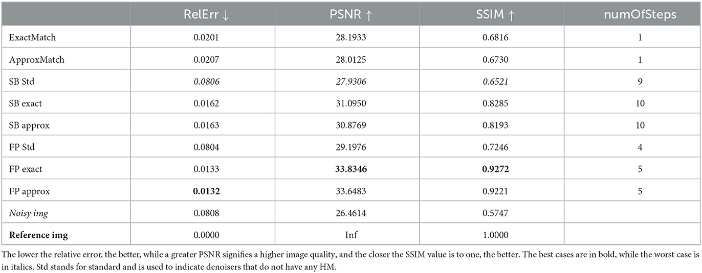
Table 1. Case 1: comparison when the matching technique is used with the original image as the target.

FIGURE 2

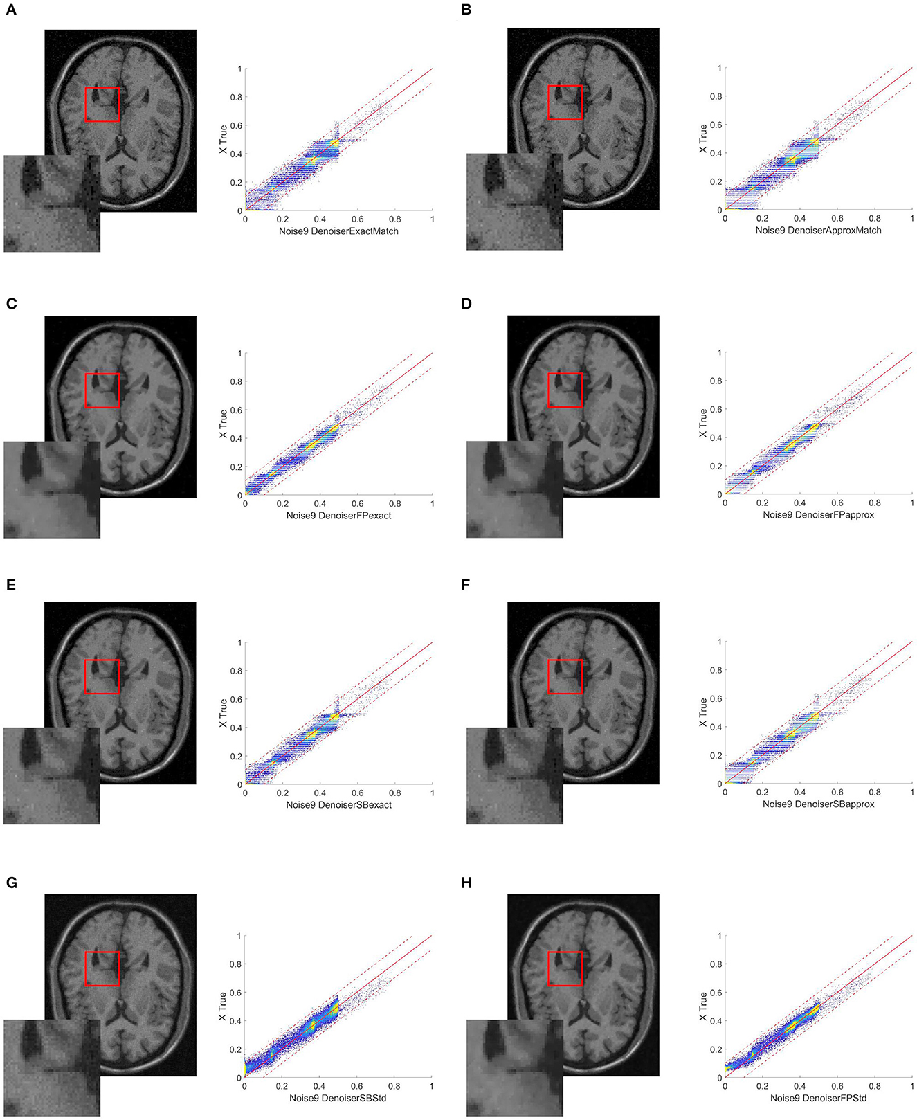
Figure 2. Resulting images when the target image is collected at a distance of -5 mm from the original image (A) ExactMatch and (B) ApproxMatch applied to the image with 9% noise. (C) FP exact and (D) FP approx denoiser applied to the image with 9% noise. (E) SB exact and (F) SB approx applied to the image with 9% noise. (G) SB standard and (H) FP standard applied to the image with 9% noise.

TABLE 2

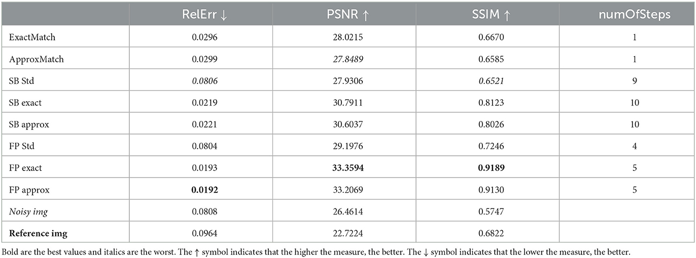
Table 2. Case 2: Comparison results, when the target image is collected at a distance of –5 mm from the original image.

FIGURE 3

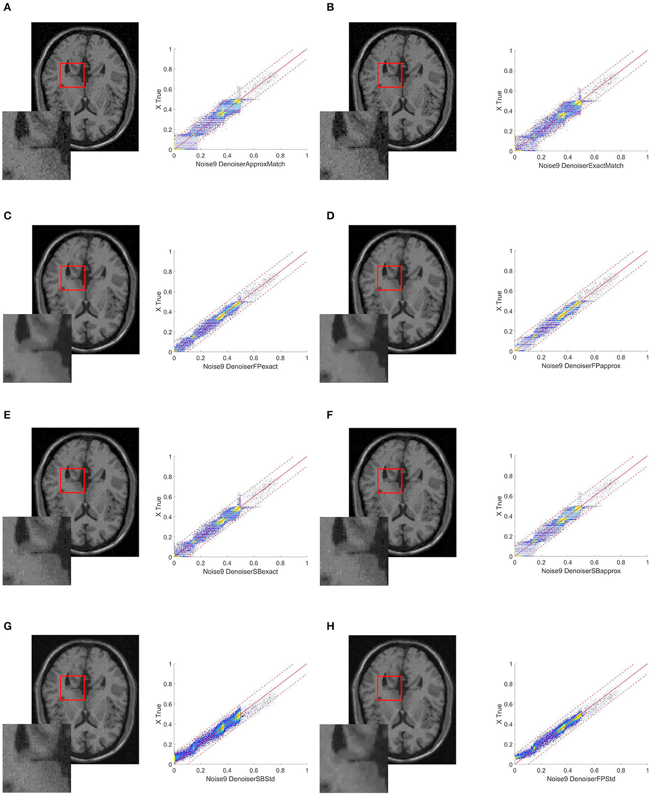
Figure 3. Resulting images when the target image is collected at a distance of –5 mm from the references, also with 3% noise. (A) ExactMatch and (B) ApproxMatch applied to the image with 9% noise. (C) FP exact and (D) FP approx denoiser applied to the image with 9% noise. (E) SB exact and (F) SB approx applied to the image with 9% noise. (G) SB standard and (H) FP standard applied to the image with 9% noise.

TABLE 3

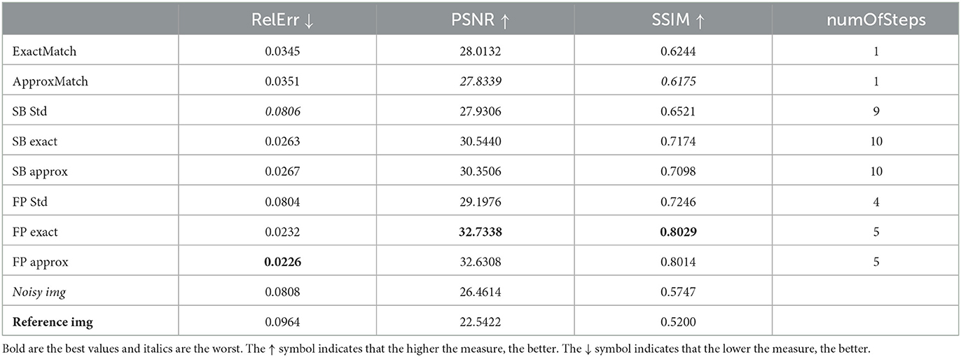
Table 3. Case 3. A more realistic case in which the target image is acquired with 9% noise at a distance of –5 mm from the original image, which has 3% noise.

FIGURE 4

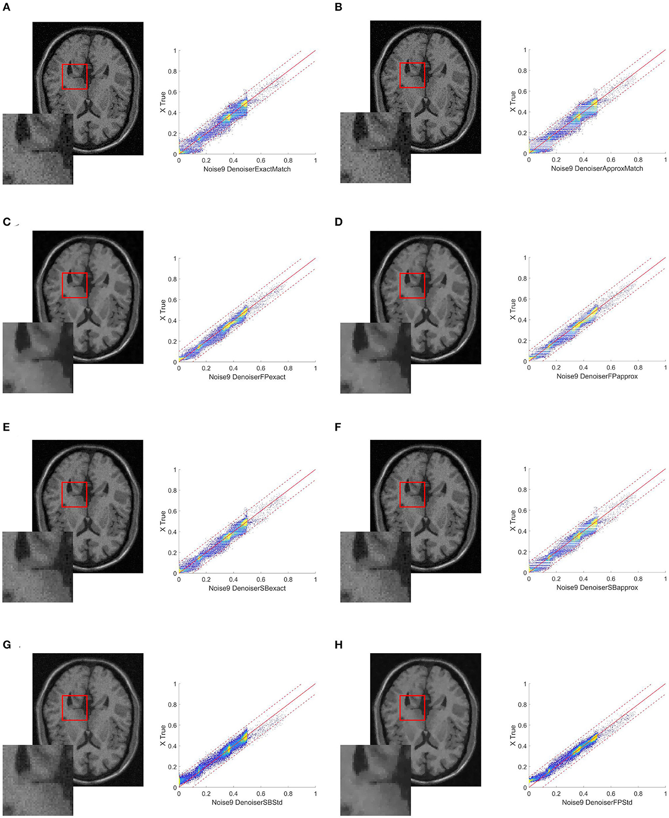
Figure 4. Resulting images when the target image is collected at a distance of +5 mm from the references, also with 3% noise. (A) ExactMatch and (B) ApproxMatch applied to the image with 9% noise. (C) FP exact and (D) FP approx denoiser applied to the image with 9% noise. (E) SB exact and (F) SB approx applied to the image with 9% noise. (G) SB standard and (H) FP standard applied to the image with 9% noise.

TABLE 4

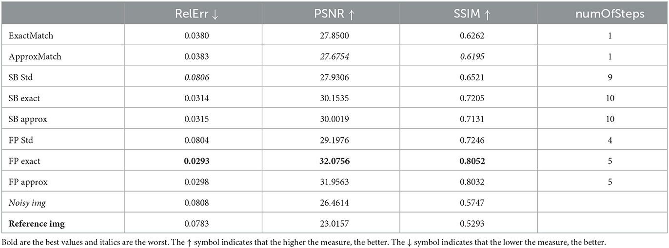
Table 4. Case 4 is another realistic case in which the target image is retrieved with 9% noise at a distance of +5 mm from the original image, which also has 3% noise.

The denoised image that outcomes will be compared to the original clean slice. This will be achieved by presenting the relative error (Rel Err), peak signal-to-noise Ratio (PSNR), and structural similarity index (SSIM). Moreover, in order to compare the outcome visually, all the histograms will have the same scale, which is shown in Figure 5D.

FIGURE 5

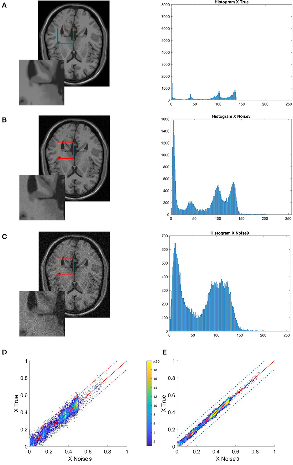
Figure 5. Sequence of images showing their respective histograms and a merged version of their histogram in 2D. (A) Ground truth. (B) Ground truth image with 3% noise. (C) Ground truth image with 9% noise. (D, E) The bi-dimensional histogram of each noisy image and the true image. The clean reference image will always be on the y-axis. The histogram patterns are more similar the closer the spots are to the diagonal of the 2D histogram.

As for the PSNR, it is mathematically defined as follows:

$PSNR=10{\log }_{10}\left(\frac{M_I^2}{MSE}\right),$

where MSE is the mean square error between the input image and the reference image, and M_I is the maximum possible pixel value of the image and is set to 1 because all BrainWeb images were re-normalized and scaled into the [0, 1] interval.

Regarding histogram matching, images are processed as either 8-bit or 16-bit, and the number of bins to match influences the results. Figure 6 depicts the results of comparing all cases to an increasing power of 2 to determine which configuration results in the lowest overall error. These results validated the selection of 2⁸ bins, which in general yielded superior results and is a common choice in image processing.

FIGURE 6

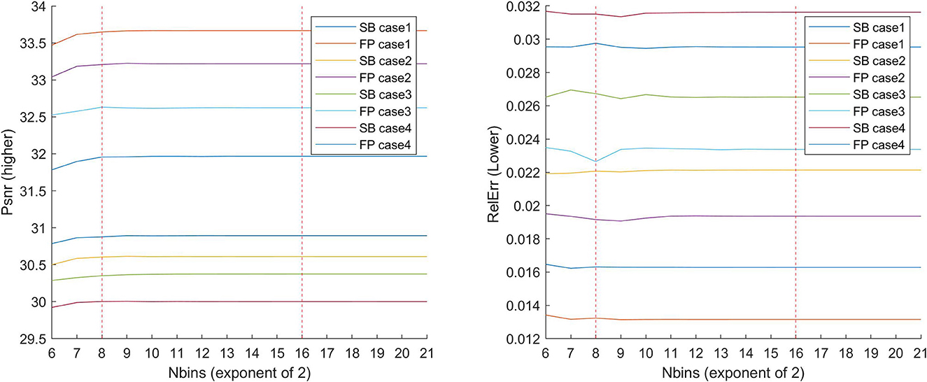
Figure 6. Graph demonstrating why we use levels of 2⁸ or 2¹⁶. We investigated what happens to the errors when the number of bins is varied for each of the cases (1,2,3, and 4) with the approximate HM presented in the study. In the literature, either 2⁸ or 2¹⁶ is commonly used. We have increased the interval and shown what happens in between. Higher levels may be a good choice for smaller values, but the main issue with using more levels is the RAM usage, which exceeds 16GB after L = 2²².

Figure 5 shows what happens to the image and its histogram when noise is added. Noise disperses values and changes peaks, as seen in a Gaussian mixture distribution by the fluctuating mean and variance of each component.

All cases will include a brain slice and a 3X zoom of the same area. Each image will be accompanied by a 2D histogram that compares the image on the y-axis to the correct reference on the x-axis. The function histogram2 generates a 2D histogram by plotting a bivariate histogram of the two input images. When looking at the histogram 2D, keep in mind that the color of a point indicates how many pixels of a specific intensity are changed from one image to another. A blue dot at the intersection of (0.4, 0.5) indicates that there are <10 points in the image described on the x-axis that should have a value of 0.5 in order to match the reference image.

3.1. Case 1: A noisy brain slice

As an initial proof of concept, we consider a brain slice with 9% of noise and assume:

1. The target histogram is known;

2. The target is the original image;

3. The matching strategy is carried out with respect to this target.

Table 1 compares the performances of the SBA and FP optimization algorithms in terms of PSNR and SSIM, relative error, and the number of iterations.

According to the results reported in Table 1, the FP (exact/approx) methods give better results than the other ones. We remind that numOfSteps is the number of denoiser iterations required to achieve the fixed tolerance of 10⁻³.

When we compare the denoisers with histogram matching to the vanilla denoisers, we can see some percentage improvements for all of the indexes used. The relative error improves the most, 79.7% from SB vanilla to SB vanilla and 83.3% between FP exact and FP vanilla; at the same time, the PSNR mildly improves 10.5% (as for the SB approx) and 16.0% (FP exact); and finally, the SSIM improves 25.6% (SB approx) or 28.4% (FP exact). In general, the exact HM outperforms the approx HM since the approx one involves a discretization of the range of values, which introduces an error that could otherwise be avoided. We also notice that FP techniques are usually superior to SB methods. Finally, based on the SSIM index, the FP exact outperforms the SB exact by 11.9%.

Figure 1 reports the results in terms of image quality and 2D histograms on the right panel. In the 2D histograms, the abscissa relates to the pixel value of the ground truth image, and the ordinate relates to one of the images in the left panel. Panel H demonstrates, for example, that most of the points are denser to the diagonal but are mostly skewed against the top-left side of the diagonal, indicating that the denoiser has correctly attempted to reduce noise by bringing the point closer to the diagonal, as shown in Figure 5, but did not have any prior knowledge of the original image. When using histogram matching, as shown in panel D, these points move to the center of the diagonal and become less dense as they move further away from the diagonal. Because histogram matching requires some level of discretization, horizontal white lines indicate that some values in the original reference image do not have a corresponding value. At the same time, the horizontal colored lines may be broader than the equivalent cleaned without matching, but the bulk of pixels that are far from the diagonal are spread closer.

3.2. Cases 2, 3, and 4: Similar real case scenarios

This subsection examines some more cases analogous to real-world scenarios.

Assuming that a cleaning and enhancement step can be done in sequence, one might start the process down the z-axis from the top to bottom-most slice and then gradually traverse through the entire z-axis. In this case, a cleaned slice from one step could be used as a subsequent slice that is 1mm distant from the previous, and because they are close to each other, given the morphology of a brain, and the structure among the various slices, while different, should be statistically similar enough to give good performance in the enhancement step. To test this hypothesis, we examine what happens when a pre-processed, cleaned slice is used as a histogram reference for the next one to process. Instead of showing the result of what happens when a contiguous ±1mm slice is used, we present the result of what happens when a 3% noise slice that is 5mm below the slice to denoise is used as a reference histogram.

In case 2, first is examined a brain slice with 9% noise, by selecting a slice that is “near” the original one as the target. Our first studies indicate that a histogram provides comparable statistical patterns up to ±5mm; as an approximation of no <0.5 for SSIM. In particular, for case 2:

1. The histogram of an image acquired at –5 mm from our original image is known;

2. The target is the acquired image;

3. The matching technique is carried-out in relation to this target.

Table 2 compares the PSNR, SSIM, relative error, and the number of iterations of the SBA and FP techniques.

In case 2, Table 2 helps us comprehend what would happen in a real situation and provides continuity to our observations as in case 1 by selecting the reference picture that is 5-mm distant from the one that was supplied. In this case, the image that serves as a reference will not be the same as the one that needs to be cleaned. As always, the SBA algorithm with λ = 4.95*10⁻² and μ = 1 has been used.

When the techniques with histogram matching are compared to the standard methods, as shown in Table 1, there is a percentage improvement in all metrics. For relative error, we have 72.6% (SB approx) and 76.2% (FP exact), the PSNR improves at 9.5% (SB approx) and 14.5% (FP exact), and finally, the SSIM improvement is 23.0% (SB approx) or 27.8% (FP exact).

In this case, we see the same pattern as in case 1, with exact matching outperforming approx matching and FP outperforming SB. We see a similar 13.1% increase in the SSIM index between the best two methods, FP and SB.

Figure 2 shows some image quality and histogram-matching results. We see that the 2D histograms relating to images processed by the denoiser in conjunction with histogram matching (panels C and D) are slightly wider than those relating to images processed by the denoiser alone (panels G and H). Although this may appear to contradict the results in Table 2, thanks to the coloring of the graph, we see a greater density of pixels best distributed along the diagonal of the histogram and thus an improvement of the expected result in accordance with the relative table.

Finally, we examine cases 3 and 4. These two cases attempt to simulate a setting that is as similar to a guanine scenario as feasible. We assume that the image to clean is rather noisy (9%) that the reference image is not perfectly clean (3% noise) and that we have a 5-mm tolerance on what the slice reference position should be, so that the two cases vary from the real location, either below (-5 mm, case 3) or above (+5 mm, case 4). Tables 3, 4 show that the improvement provided by the FP exact and FP approx methods is consistent with the previous cases. The method's robustness is even more noticeable because the results are obtained from reference images with an SSIM index (compared to the clean image) lower than the SSIM index of the image with noise at 3%. In other words, the improvement provided by the FP exact and FP approx approaches is kept, while the method's resilience is enhanced. This can also be seen in Figures 3, 4. From these images, it is visible how much better the HM distributes the pixels in the histogram than the denoiser alone. For example, when observing the square [0 0.2] in panel H in comparison to the same square in panels C and D, the reader can see a yellow spot indicating a higher density of pixels, which in panel H is completely above the diagonal, whereas when the denoiser is combined with the HM, this pigment is distributed equally on the diagonal. Another thing to notice is that the cut at 0.5 is perfectly vertical when simply the denoiser is used; however, the dye at the cut is also spread horizontally in the C or D panels. This is mathematically measured with higher PSNR and SSIM values as well as lower relative error values because these metrics, by analyzing the similarity with the reference image, are actually evaluating how close the majority of pixels are to the diagonal, i.e., a perfect match.

We also see improvements in all metrics when comparing standard denoising methods to HM ones.

Relative error improvement can be as high as 60.9% (SB approx in case 4) or 72.1% (FP exact in case 3); for PSNR, we have a 7.4% improvement for the SB approx in case 3, or 12.2% for the FP exact in case 4; and for the SSIM, we have a good improvement of 8.8% (SB approx in case 3) and 12.0% (FP exact in case 4).

In cases 3 and 4, we see the same pattern as in the previous cases, namely, that exact matching is better than approximate matching and FP is better than SB. We see a similar 12.0% increase in the SSIM index from the second-best method, the SB exact, to the first-best method, the FP exact.

4. Discussion

This final section summarizes the results and then points out the way to further research. The dual-stage procedure that combines denoising and enhancement is superior to the single two solutions. Further research could include an extension to Gaussian mixture models (GMMs) and, as a result, the use of machine learning approaches.

4.1. Discussion on the results

As can be seen from Tables 1–4, there are improvements in the two-step procedure with an increment of one iteration. Overall, you get better results when using the same slice type in the histogram that corresponds to Table 1, as you might expect, but relative to each case, you get minimal SSIM improvement of 8.6%, of the relative error of 60.0% and the PSNR index of 7.4% also obtained using other sections (noised) as a reference of the histogram. There are minor differences between different histogram matching algorithms, but it is worth noting that the target image makes a significant difference.

The difference can be noted in the type of algorithm used, but more importantly, in the target histogram. In these example cases, we are using completely different types of target images, the ground truth image, and noisy slices. As might be expected by using the same type of slice in the histogram matching, there are better results, but good results are obtained even if one uses as reference histogram slices that are within 5mm. Although the two histogram matching algorithms differ significantly, the end effect on the metrics we employed is fairly minimal. However, it is worth noting that the target image makes a significant difference in lowering the relative error and increasing PSNR and SSIM.

Figures 1–4 also show what happens to the image and its histogram when noise is removed with a denoiser. The denoiser tries to smooth the spikes of the histogram, without knowing in which direction to improve the histogram. This observation brought the authors to investigate histograms, and in particular, a useful tool is histogram specification (or matching). In this scenario, the proposed methodology can easily bring to design novel approaches for MRI enhancement and denoising. The basic idea is to exploit more in-depth the MRI domain more, i.e., information from the specific part of the body, and use such information for near slices as they are cleaned.

Limitations can be addressed to the difficulty of setting the prior image from which to extrapolate the most suitable histogram. Furthermore, the convergence of the dual-stage algorithm has yet to be mathematically proven, despite experimental tests demonstrating convergence within different parameters.

The correct number of bins into which the histogram is divided has been investigated, as illustrated in Figure 6. When determining the best number of bins, remember to consider the memory limits of the computer in use, as once the 2²² bins are exceeded, the algorithm requires more than 16GB of RAM. Taking this into consideration, a varying bin-width phase based on the specific domain (brain, knee, etc.) could be considered. Several histogram matching algorithms, particularly non-exact ones or those that attempt to add a small amount of noise to each pixel's intensity value, can be investigated further to improve the obtained results.

Finally, in all of our case studies, the FP method outperforms the SB method; however, this does not always hold true. On the contrary, the literature has examples of SB methods producing results that are superior to FP methods. In Kim and Yun [56], for example, the fixed-point technique for the TV-L2 model performs worse than the corresponding split Bregman method, whereas the fixed-point-like approach for the TV-L2 model performs almost as well as the corresponding split Bregman method, depending on the exact implementation.

4.2. Conclusion and further work

The proposed model can become a framework for techniques blending denoising and enhancement. Enhancement using histogram matching can be further improved by gathering some statically relevant information of typical histograms of a specific part of the body; in fact, this can be successively extended with the use of Gaussian Mixtures Models (GMMs), a convex combination of Gaussian densities. This has led the authors to study how machine learning can be used to find the most similar histogram in a database of statistically relevant histograms. Other techniques can yield to deal with MRIs containing statically relevant artifacts not coming from noise.

An interesting approach is to combine the denoising strategies with a post-processing technique based on histogram matching. In general, it is possible to create a dictionary of images that contains the intensity distribution of MRI data based on a suitable model describing the anatomical parts of a body as a target, such as brain slices. The target is an a priori information and in our case, the image histograms and the most similar histogram must be searched [57]. The knowledge hidden in a 3D MRI dataset can be selected by using machine learning tools to extract the correct target. A dictionary of targets approach framework can be inspired by some recent work in the literature [57, 58]. It is possible to use the parameters from a pre-learned GMM; then, in terms of matching strategy, we can consider comparing histograms based on GMM. Actually, to model the complex data distribution, a GMM is frequently employed, and the expectation-maximization (EM) algorithm is frequently used to create the mixture model [59]. Ma et al. [60] recently proposed a feature-guided GMM for robust feature matching that is capable of handling both rigid and non-rigid deformations. In fact, feature matching is a wide research topic in image retrieval, with the goal of creating accurate correspondences between two image feature sets [61].

The dual-stage algorithm is another research topic. The first open research study is to prove mathematically its convergence and improvement. Another investigation could include expanding the dual-stage algorithm to a multi-stage algorithm. One approach would be to apply histogram matching to each step of the denoising algorithm by altering the minimization problem (in our preliminary test, this approach did not give good results). Another option is to use matching after reaching a certain tolerance and then restart the denoiser to achieve a lower tolerance. Next, the multi-stage approach could be made by enhancing the image with HM to only certain areas of the brain. Moreover, further denoiser filters can be investigated such as the median filter instead of the total variation one, or use as histogram enhancement the contrast limited adaptive histogram equalization (CLAHF), combined with a matching procedure. The implementations should then be done in Python, as this language and all of its libraries can be used to build a larger machine learning framework based on a look-up table of GMM statically relevant brain slices. In future work, the histogram to match would be a synthetic GMM-based histogram; nonetheless, in this proof-of-concept work, this study demonstrated how matching behaves with various histograms by gradually simulating a real-world scenario.

Finally, all of these tests should be carried out in a more realistic environment. For example, the technique can be tested against the BCU Imaging Biobank, a non-profit biorepository dedicated to the collection and retrieval of diagnostic images, derived descriptors, and clinical data [62].

Our method improved overall image quality for all sequences and outperformed in all individual categories; using this dual-stage method, homogeneous objects/tumors in medical images can be segmented. Finally, as preprocessing medical images is a de facto standard first step, our model can be used in almost all deep learning pipelines for medical image segmentation.

Data availability statement

The original contributions presented in the study are included in the article/supplementary material, further inquiries can be directed to the corresponding authors.

Author contributions

VS, LA, and SC contributed to the conception and design of the study. VS, DM, AB, and LA developed the code. VS, LA, AB, and SC performed the mathematical analysis. VS wrote the first draft of the manuscript. DM, AB, LA, and SC wrote sections of the manuscript. All authors contributed to the manuscript revision, read, and approved the submitted version.

Funding

SC was partially supported by INdAM-GNCS. This research has been accomplished within the two Italian research groups on approximation theory: RITA and UMI-T.A.A.

Acknowledgments

The authors would like to thank Dr. Laura Antonelli for her assistance and guidance in TV-ROF denoisers. Dr. Preety Baglat was extremely helpful in reviewing and revising the manuscript. Finally, the authors thank the reviewers whose comments helped us strengthen and improve the manuscript.

Conflict of interest

The authors declare that the research was conducted in the absence of any commercial or financial relationships that could be construed as a potential conflict of interest.

Publisher's note

All claims expressed in this article are solely those of the authors and do not necessarily represent those of their affiliated organizations, or those of the publisher, the editors and the reviewers. Any product that may be evaluated in this article, or claim that may be made by its manufacturer, is not guaranteed or endorsed by the publisher.

References

1. Curtis WA, Fraum TJ, An H, Chen Y, Shetty AS, Fowler KJ. Quantitative MRI of diffuse liver disease: current applications and future directions. Radiology. (2019) 290:23–30. doi: 10.1148/radiol.2018172765

PubMed Abstract | CrossRef Full Text | Google Scholar

2. Zanfardino M, Franzese M, Pane K, Cavaliere C, Monti S, Esposito G, et al. Bringing radiomics into a multi-omics framework for a comprehensive genotype-phenotype characterization of oncological diseases. J Transl Med. (2019) 17:337. doi: 10.1186/s12967-019-2073-2

PubMed Abstract | CrossRef Full Text | Google Scholar

3. Aiello M, Cavaliere C, DAlbore A, Salvatore M. The challenges of diagnostic imaging in the era of big data. J Clin Med. (2019) 8:316. doi: 10.3390/jcm8030316

PubMed Abstract | CrossRef Full Text | Google Scholar

4. Aiello M, Esposito G, Pagliari G, Borrelli P, Brancato V, Salvatore M. How does DICOM support big data management? Investigating its use in medical imaging community. Insights Into Imaging. (2021) 12:164. doi: 10.1186/s13244-021-01081-8

PubMed Abstract | CrossRef Full Text | Google Scholar

5. Hadjidemetriou E, Grossberg MD, Nayar SK. Multiresolution histograms and their use for recognition. IEEE Trans Pattern Anal Mach Intell. (2004) 26:831–47. doi: 10.1109/TPAMI.2004.32

PubMed Abstract | CrossRef Full Text | Google Scholar

6. Kociołek M, Strzelecki M, Obuchowicz R. Does image normalization and intensity resolution impact texture classification? Comput Med Imaging Graphics. (2020) 81:101716. doi: 10.1016/j.compmedimag.2020.101716

PubMed Abstract | CrossRef Full Text | Google Scholar

7. Mohan J, Krishnaveni V, Guo Y. A survey on the magnetic resonance image denoising methods. Biomed Signal Process Control. (2014) 9:56–69. doi: 10.1016/j.bspc.2013.10.007

CrossRef Full Text | Google Scholar

8. Bazin PL, Alkemade A, van der Zwaag W, Caan M, Mulder M, Forstmann BU. Denoising high-field multi-dimensional MRI with local complex PCA. Front Neurosci. (2019) 13:1066. doi: 10.3389/fnins.2019.01066

PubMed Abstract | CrossRef Full Text | Google Scholar

9. Ouahabi A. A review of wavelet denoising in medical imaging. In: 2013 8th International Workshop on Systems, Signal Processing and their Applications (WoSSPA). (2013). p. 19–26. doi: 10.1109/WoSSPA.2013.6602330

CrossRef Full Text | Google Scholar

10. Benfenati A, Ruggiero V. Image regularization for Poisson data. J Phys. (2015) 657:012011. doi: 10.1088/1742-6596/657/1/012011

CrossRef Full Text | Google Scholar

11. Benfenati A, Ruggiero V. Inexact Bregman iteration for deconvolution of superimposed extended and point sources. Commun Nonlinear Sci Num Simulat. (2015) 20:882–96. doi: 10.1016/j.cnsns.2014.06.045

CrossRef Full Text | Google Scholar

12. Hammernik K, Würfl T, Pock T, Maier A. A deep learning architecture for limited-angle computed tomography reconstruction. In:Maier-Hein gF Klaus Hermann, Deserno gL Thomas Martin, Handels H, Tolxdorff T, , editors. Bildverarbeitung für die Medizin 2017 Informatik aktuell. Berlin; Heidelberg: Springer (2017). p. 92–7.

PubMed Abstract | Google Scholar

13. Lanza A, Morigi S, Sgallari F. Convex image denoising via non-convex regularization with parameter selection. J Math Imaging Vis. (2016) 56:195–220. doi: 10.1007/s10851-016-0655-7

CrossRef Full Text | Google Scholar

14. Morigi S, Reichel L, Sgallari F. Fractional Tikhonov regularization with a nonlinear penalty term. J Comput Appl Math. (2017) 324:142–54. doi: 10.1016/j.cam.2017.04.017

CrossRef Full Text | Google Scholar

15. De Asmundis R, di Serafino D, Landi G. On the regularizing behavior of the SDA and SDC gradient methods in the solution of linear ill-posed problems. J Comput Appl Math. (2016) 302:81–93. doi: 10.1016/j.cam.2016.01.007

CrossRef Full Text | Google Scholar

16. Zanetti M, Ruggiero V, Miranda M Jr. Numerical minimization of a second-order functional for image segmentation. Commun Nonlinear Sci Num Simulat. (2016) 36:528–48. doi: 10.1016/j.cnsns.2015.12.018

PubMed Abstract | CrossRef Full Text | Google Scholar

17. Lustig D, Martonosi M. Reducing GPU offload latency via fine-grained CPU-GPU synchronization. In: 2013 IEEE 19th International Symposium on High Performance Computer Architecture (HPCA). Shenzhen: IEEE (2013). p. 354–65.

Google Scholar

18. Quan TM, Han S, Cho H, Jeong WK. Multi-GPU reconstruction of dynamic compressed sensing MRI. In:Navab N, Hornegger J, Wells WM, Frangi AF, , editors. Medical Image Computing and Computer-Assisted Intervention - MICCAI 2015 Lecture Notes in Computer Science. Cham: Springer International Publishing (2015). p. 484–92.

Google Scholar

19. Luo E, Chan SH, Nguyen TQ. Adaptive image denoising by mixture adaptation. IEEE Trans Image Process. (2016) 25:4489–503. doi: 10.1109/TIP.2016.2590318

PubMed Abstract | CrossRef Full Text | Google Scholar

20. Schob S, Meyer HJ, Dieckow J, Pervinder B, Pazaitis N, Höhn AK, et al. Histogram analysis of diffusion weighted imaging at 3T is useful for prediction of lymphatic metastatic spread, proliferative activity, and cellularity in thyroid cancer. Int J Mol Sci. (2017) 18:E821. doi: 10.3390/ijms18040821

PubMed Abstract | CrossRef Full Text | Google Scholar

21. Senthilkumaran N, Thimmiaraja J. Histogram equalization for image enhancement using MRI brain images. In: 2014 World Congress on Computing and Communication Technologies. (2014). p. 80–3. doi: 10.1109/WCCCT.2014.45

CrossRef Full Text | Google Scholar

22. Grossberg MD, Nayar SK. Determining the camera response from images: what is knowable? IEEE Trans Pattern Anal Mach Intell. (2003) 25:1455–67. doi: 10.1109/TPAMI.2003.1240119

CrossRef Full Text | Google Scholar

23. Gonzalez RC, Woods RE. Digital Image Processing. Pearson Education (2011).

24. Edeler T, Ohliger K, Hussmann S, Mertins A. Time-of-flight depth image denoising using prior noise information. In: IEEE 10th International Conference on Signal Processing Proceedings. Beijing: IEEE (2010). p. 119–22.

Google Scholar

25. Campagna R, Crisci S, Cuomo S, Marcellino L, Toraldo G. Modification of TV-ROF denoising model based on split Bregman iterations. Appl Math Comput. (2017) 315:453–67. doi: 10.1016/j.amc.2017.08.001

CrossRef Full Text | Google Scholar

26. Block KT, Uecker M, Frahm J. Undersampled radial MRI with multiple coils. Iterative image reconstruction using a total variation constraint. Magn Reson Med. (2007) 57:1086–98. doi: 10.1002/mrm.21236

PubMed Abstract | CrossRef Full Text | Google Scholar

27. Castellano M, Ottaviani D, Fontana A, Merlin E, Pilo S, Falcone M. Improving resolution and depth of astronomical observations via modern mathematical methods for image analysis. ArXiv:1501.03999 [astro-ph] (2015). doi: 10.48550/arXiv.1501.03999

CrossRef Full Text | Google Scholar

28. Roscani, V, Tozza, S, Castellano, M, et al. A comparative analysis of denoising algorithms for extragalactic imaging surveys. A&A. (2020) 643:A43. doi: 10.1051/0004-6361/201936278

CrossRef Full Text | Google Scholar

29. Rudin LI, Osher S, Fatemi E. Nonlinear total variation based noise removal algorithms. Phys D. (1992) 60:259–68. doi: 10.1016/0167-2789(92)90242-F

CrossRef Full Text | Google Scholar

30. Chambolle A, Levine SE, Lucier BJ. Some variations on total variation-based image smoothing. In: Working Paper or Preprint. (2009). Available online at: https://hal.science/hal-00370195

Google Scholar

31. Alliney S. A property of the minimum vectors of a regularizing functional defined by means of the absolute norm. IEEE Trans Signal Process. (1997) 45:913–7. doi: 10.1109/78.564179

CrossRef Full Text | Google Scholar

32. Nikolova M. A variational approach to remove outliers and impulse noise. J Math Imaging Vis. (2004) 20:99–120. doi: 10.1023/B:JMIV.0000011920.58935.9c

CrossRef Full Text | Google Scholar

33. Goldstein T, Osher S. The split bregman method for L1-regularized problems. SIAM J Imaging Sci. (2009) 2:323–43. doi: 10.1137/080725891

PubMed Abstract | CrossRef Full Text | Google Scholar

34. Condat L. Discrete total variation: new definition and minimization. SIAM J Imaging Sci. (2017) 10:1258–90. doi: 10.1137/16M1075247

CrossRef Full Text | Google Scholar

35. González G, Kolehmainen V, Seppänen A. Isotropic and anisotropic total variation regularization in electrical impedance tomography. Comput Math Appl. (2017) 74:564–76. doi: 10.1016/j.camwa.2017.05.004

CrossRef Full Text | Google Scholar

36. Lou Y, Zeng T, Osher S, Xin J. A weighted difference of anisotropic and isotropic total variation model for image processing. SIAM J Imaging Sci. (2015) 8:1798–823. doi: 10.1137/14098435X

CrossRef Full Text | Google Scholar

37. Chambolle A, Lions PL. Image recovery via total variation minimization and related problems. Numer Math. (1997) 76:167–88. doi: 10.1007/s002110050258

CrossRef Full Text | Google Scholar

38. Antonelli L, De Simone V, Viola M. Cartoon-texture evolution for two-region image segmentation. Comput Optimizat Appl. (2022) 84:5–26. doi: 10.1007/s10589-022-00387-7

CrossRef Full Text | Google Scholar

39. Setzer S, Steidl G, Teuber T. Deblurring poissonian images by split Bregman techniques. J Visual Commun Image Represent. (2010) 21:193–9. doi: 10.1016/j.jvcir.2009.10.006

CrossRef Full Text | Google Scholar

40. Vogel CR, Oman ME. Iterative methods for total variation denoising. SIAM J Sci Comput. (1996) 17:227–38. doi: 10.1137/0917016

CrossRef Full Text | Google Scholar

41. Boyd S, Parikh N, Chu E, Peleato B, Eckstein J. Distributed optimization and statistical learning via the alternating direction method of multipliers. Found Trends Mach Learn. (2011) 3:1–122. doi: 10.1561/9781601984616

CrossRef Full Text | Google Scholar

42. Afonso MV, Bioucas-Dias JM, Figueiredo MA. Fast image recovery using variable splitting and constrained optimization. IEEE Trans Image Process. (2010) 19:2345–56. doi: 10.1109/TIP.2010.2047910

PubMed Abstract | CrossRef Full Text | Google Scholar

43. Goldstein T, Bresson X, Osher S. Geometric applications of the split Bregman method: segmentation and surface reconstruction. J Sci Comput. (2010) 45:272–93. doi: 10.1007/s10915-009-9331-z

CrossRef Full Text | Google Scholar

44. Tai XC, Wu C. Augmented Lagrangian method, dual methods and split Bregman iteration for ROF model. In: Scale Space and Variational Methods in Computer Vision. (2009). p. 502–13.

Google Scholar

45. Getreuer P. Rudin-Osher-Fatemi total variation denoising using split Bregman. Image Process Line. (2012) 2:74–95. doi: 10.5201/ipol.2012.g-tvd

CrossRef Full Text | Google Scholar

46. Li W, Li Q, Gong W, Tang S. Total variation blind deconvolution employing split Bregman iteration. J Vis Commun Image Represent. (2012) 23:409–17. doi: 10.1016/j.jvcir.2011.12.003

CrossRef Full Text | Google Scholar

47. Bush J. Bregman algorithms (Senior thesis). University of California, Santa Barbara (2011).

Google Scholar

48. Embrechts P, Hofert M. A note on generalized inverses. Math Methods Operat Res. (2013) 77:423–32. doi: 10.1007/s00186-013-0436-7

CrossRef Full Text | Google Scholar

49. Coltuc D, Bolon P, Chassery JM. Exact histogram specification. IEEE Trans Image Process. (2006) 15:1143–52. doi: 10.1109/TIP.2005.864170

PubMed Abstract | CrossRef Full Text | Google Scholar

50. Coltuc D, Bolon P. Strict ordering on discrete images and applications. In: Proceedings 1999 International Conference on Image Processing (Cat. 99CH36348). Vol. 3 (1999). p. 150–3. doi: 10.1109/ICIP.1999.817089

CrossRef Full Text | Google Scholar

51. Nikolova M, Steidl G. Fast ordering algorithm for exact histogram specification. IEEE Trans Image Process. (2014) 23:5274–83. doi: 10.1109/TIP.2014.2364119

PubMed Abstract | CrossRef Full Text | Google Scholar

52. Nikolova M, Wen YW, Chan R. Exact histogram specification for digital images using a variational approach. J Math Imaging Vis. (2013) 46:309–25. doi: 10.1007/s10851-012-0401-8

PubMed Abstract | CrossRef Full Text | Google Scholar

53. Bevilacqua A, Azzari P. A high performance exact histogram specification algorithm. In: ICIAP. IEEE Computer Society. Modena: IEEE (2007). p. 623–8.

Google Scholar

54. Semechko A. Exact histogram equalization and specification (2019).

55. Brain Web,. (2022). Simulated Brain Database, Mcconnell Brain Imaging Centre, Montreal Neurological Institute, McGill University. Available online at: http://brainweb.bic.mni.mcgill.ca/brainweb/

56. Kim KS, Yun JH. Image restoration using a fixed-point method for a TVL2 regularization problem. Algorithms. (2020) 13:1. doi: 10.3390/a13010001

CrossRef Full Text | Google Scholar

57. Macke S, Zhang Y, Huang S, Parameswaran A. Adaptive sampling for rapidly matching histograms. Proc VLDB Endowment. (2018) 11:1262–75. doi: 10.14778/3231751.3231753

CrossRef Full Text | Google Scholar

58. Grauman K, Darrell T. The pyramid match kernel: discriminative classification with sets of image features. In: Tenth IEEE International Conference on Computer Vision (ICCV'05) Volume 1. Beijing: IEEE (2005). p. 1458–65.

59. Peng J, Shao Y, Sang N, Gao C. Joint image deblurring and matching with feature-based sparse representation prior. Pattern Recogn. (2020) 103:107300. doi: 10.1016/j.patcog.2020.107300

CrossRef Full Text | Google Scholar

60. Ma J, Jiang X, Jiang J, Gao Y. Feature-guided Gaussian mixture model for image matching. Pattern Recogn. (2019) 92:231–45. doi: 10.1016/j.patcog.2019.04.001

PubMed Abstract | CrossRef Full Text | Google Scholar

61. Asheri H, Hosseini R, Araabi BN. A new EM algorithm for flexibly tied GMMs with large number of components. Pattern Recogn. (2021) 114:107836. doi: 10.1016/j.patcog.2021.107836

CrossRef Full Text | Google Scholar

62. Esposito G, Pagliari G, Randon M, Mirabelli P, Lavitrano M, Aiello M, et al. BCU imaging biobank, an innovative digital resource for biomedical research collecting imaging and clinical data from human healthy and pathological subjects. Open J Bioresour. (2021) 8:4. doi: 10.5334/ojb.72

CrossRef Full Text | Google Scholar