Deep Image Prior for medical image denoising, a study about parameter initialization

Convolutional Neural Networks are widely known and used architectures in image processing contexts, in particular for medical images. These Deep Learning techniques, known for their ability to extract high-level features, almost always require a labeled dataset, a process that can be computationally expensive. Most of the time in the biomedical context, when images are used they are noisy and the ground-truth is unknown. For this reason, and in the context of Green Artificial Intelligence, recently, an unsupervised method that employs Convolutional Neural Networks, or more precisely autoencoders, has appeared in the panorama of Deep Learning. This technique, called Deep Image Prior (DIP) by the authors, can be used in areas such as denoising, superresolution, and inpainting. Starting from these assumptions, this work analyses the robustness of these networks with respect to different types of initialization. First of all, we analyze the different types of parameters: related to the Batch Norm and the Convolutional layers. For the results, we focus on the speed of convergence and the maximum performance obtained. However, this paper aims to apply acquired information on Computer Tomography noised images. In fact, the final purpose is to test the best initializations of the first phase on a phantom image and then on a real Computer Tomography one. In fact, Computer Tomography together with Magnetic Resonance Imaging and Positron Emission Tomography are some of the diagnostic tools currently available to neuroscientists and oncologists. This work shows how initializations affect final performances and, in addition, how they should be used in the medical image reconstruction field. The section on numerical experiments shows results that on the one hand confirm the importance of a good initialization to obtain fast convergence and high performance; on the other hand, it shows how the method is robust to the processing of different image types: natural and medical. Not a single good initialization is discovered, but many of them could be chosen, according to specific necessities of the single problem.

1. Introduction

X-ray Computed Tomography (CT) [1] is a fundamental imaging method in clinical routine. Moreover, it is applied also in other areas such as engineering and arts, due to its ability to extract information about the inner structure of an object. Computed Tomography was developed in 1970 as the first non-invasively method able to acquire images of the inside of the human body that were not biased by the superposition of distinct anatomical elements. It was considered an enormous step during the 70 s.

Nowadays, medical CT research is mostly focused on developing safer protocols and reducing the radiation dose. Not only would it be of interest to medicine, but it also would prevent damage to materials science and cultural heritage. One possible method in order to do that is to minimize the number of X-rays projection, with the purpose of a sparse tomography (or sparse-view). In traditional, non-sparse, CT about one-thousand's projections are executed over the 360° trajectory. On contrary, sparse tomography requires a wider angular step between two adjacent scans. In addition, in special cases where there are practical limitations, the X-ray source could walk only a semi-circular path. Therefore, the resulting images may probably be incomplete, and streaking artifacts will corrupt them.

For this reason, the main problem of CT is the reconstruction of an object from its projections. This paper aims to artifacts removal on tomographic image reconstructions.

Tomographic image reconstruction is one of the most important challenges in the fields of mathematical oncology and neuroscience. In fact, mathematical advanced tools could be concretely applied in order to improve medical diagnosis. Deep Convolutional Neural Networks (DCNNs) have become a popular tool for inverse image reconstruction, image generation, and restoration, setting the state-of-the-art for these problems. Many applications exists, such as Adversarial Networks [2], Variational Autoencoders [3], Direct Pixelwise Minimization [4], Deep Image Prior (DIP) [5], Image Super Resolution [6].The purpose of this paper is to improve CT images' quality, exploiting a particular Autoencoders' skill. It is the ability of learning, given an image, first structures and, then, noise. We think this could be an important resource if exploited in image reconstruction tasks.

Despite their good performances, the learning process of Deep Neural Networks (DNN) has not yet been explained in detail. How they generalize depends on different aspects, some of them still unknown. One significant element of the training process is the parameters initialization choice. Since DNNs are strongly non-convex and non-linear, they may have multiple local minima, hence finding a good initialization of the parameters is critical in order to achieve good performances and limited training time. This paper aims to a better understanding of how initialization affects on performance and training time of an Autoencoder, or more in general a Deep Convolutional Neural Network.

Through this experimental study, we try to depict the influence of the initialization techniques on performances and training time. Finding an appropriate range for the initial weights could really change the final results.

The chosen Autoencoder [5, 7] belongs to the DIP category, and it is prone to semi-convergence. Regarding the choice of the CNN architecture, in particular the autoencoder architecture, in this work we fix it as one of the networks proposed in Ulyanov et al. [5], that is an autoencoder with five downsampling and five bilinear upsampling layers with convolutional skip connections. This phenomenon of semi-convergence is based on the fact that the Autoencoder, trained for a denoise-image reconstruction on a single image, first rebuilds the cleaned image, then adds noise. As stated by Ulyanov et al., “In other words, the parametrization offers high impedance to noise and low impedance to signal” [5]. For this reason, convergence, on the ground-truth image, is obtained before the end of the training process and, after this peak, the Autoencoders learn not only the real image, but the image plus noise. For this reason, after a certain number of epochs the performance decrease. The convergence is evaluated by computing the Peak Signal-to-Noise Ratio (PSNR) and saving the best of PSNR. We have chosen this particular problem because evaluating its convergence point and the optimal performance is clear.

In order to obtain experimental results, four initialization strategies were differently permuted for weights and biases of Convolution layers and weights and biases of Batch Normalization (BN), for a total of 4⁴ = 256 initialization combinations per image.

Therefore, we investigated the robustness of these particular Autoencoder architectures, observing how significant the initialization impact on both criteria is, in terms of performance values and convergence time.

This particular architecture, explained in detail in section 3, is used in many applications. While all the hyperparameters were fixed, the architecture is initialized in different ways.

First, initialization experiments are trained on real RGB images, not concerning the medical field. Second, the same experiments are repeated on a gray-scale phantom image (with two different resolutions). In addition, both qualitative and quantitative analyses have been reported. Finally, the best initialization selected from previous experiments is used for the last autoencoder training, computed on a real chest CT medical image representing a section of two lungs on a patient affected by COVID-19 [8]. In this conclusive phase, due to the absence of ground-truth in real medical images, a comparative analysis is provided, but not the quantitative one.

To sum up, contributions of this paper are:

• To improve the autoencoder model taken from Ulyanov et al. [5] through different initialization methods.

• To use this specific autoencoder in a different field, CT images.

• To combine new information from different images, not medical-related, and use them in an state-of-the-art medical problem such as image reconstruction.

The reminder of this paper is organized as follows. Section 2 presents the state-of-the-art initialization strategies and past experimental studies about them. Experimental details about the methods used, with specific motivations, are presented in section 3. The obtained analysis and results on the first part are discussed in section 4. In the end, concluding remarks are given.

2. Related Work

A key to a successful DNN implementation could be improving the generalization ability. In order to achieve this, during the implementation different aspects have to be considered. The purpose of this paper consists in exploring how initialization affects the performance of a Convolutional Autoencoder and how, in this specific case, initialization and robustness are related.

The contribution of this paper is mostly experimental, since it is quite utopian to draw theoretical results on the effect of different initializations in the non-convex and stochastic framework of the neural networks. Even in the standard variational deterministic case, in order to obtain convergence results for non-convex objective functions very strong conditions are imposed on either the objective function and the initialization [see e.g., the Capture Theorem in Bertsekas [9] to guarantee convergence to a minimum point] and/or the optimization algorithm itself [see e.g., the negative curvature directions methods in Gould et al. [10] for convergence to second order stationary points]. On the other hand, Goodfellow et al. themselves in their famous book [11] state that “Modern initialization strategies are simple and heuristic. Designing improved initialization strategies is a difficult task because neural network optimization is not yet well-understood. […] Our understanding of how the initial point affects generalization is especially primitive, offering little to no guidance for how to select the initial point.”

Different papers have explored parameters initialization in DNNs, in order to improve specific NN performances and contrast vanishing/exploding gradient problems. Especially, the most widely faced problem is initialization for classification models, whereas our paper is focused on initialization in Autoencoders. Recently many initialization methods were compared and proposed, for example in the following work, where the authors apply different types of initialization to datasets that are well-known in the literature. In Mishkin and Matas [12] different initializations for classification cases are analyzed, particularly with datases: CIFAR10, CIFAR100, and MNIST. In Aghajanyan [13], the author applied different initializations to IMDB Movie Review, a binary sentiment analysis dataset consisting of 50, 000 reviews from the Internet Movie Database (IMDb). In Arpit et al. [14], a particular family of CNNs is considered, instead of a particular dataset, thus this work analyzes how different initializations affect the training phase of the ResNet (Residual Network) family.

Due to the non-convexity of DNN problems, the initial point is fundamental. On the other hand, a too large or too small parameter scale could lead to information vanishing or exploding, especially in very DNNs (more than eight layers), when the backpropagation is applied to a long chain of gradients. Indeed, initialization has a substantial impact on the final performance of the networks and on the convergence time. We will prove that initialization plays a key-role, also in Deep Learning Explainability, because it affects all the training processes and in particular the convergence process. Since extensive literature about initialization schemes exists, we resume in this paper some of the most widely used initialization strategies.

In the literature three main initialization techniques have been identified: Data Independent, Data Dependent [15], and Pre-Training approach. In our case, the problem addressed is an unsupervised one, thus not adapted to Pre-Training techniques. Moreover, since the purpose of our experimental study is an analysis of generalization properties, Data Dependent techniques were excluded.

Recent DNNs, especially CNNs [16], are usually initialized by random weights with a Gaussian or Uniform distribution. With a fixed standard deviation, very deep models have difficulties to converge without techniques that avoid exploding gradient, therefore we choose them combined with a BN process, to reduce the problem.

Also more elaborated initialization strategies exist, which tried to solve the vanishing/exploding gradient.

Xavier initialization was proposed by Glorot and Bengio [17] and consists in a Gaussian distribution, where the standard deviation is not fixed, but it depends on the number of input and output channels of the layers. The idea is to investigate the variance of the responses in each layer. This method has a big constraint: it assumes the non-linearity between layers, imposing

$n_{l}Var\left[{\omega }_l\right]=1$

where n_l is the number of connections of a response in the l-th layer and ω_l represents each element of the weight matrix W_l. Although the restrictive assumption, this initialization has promising results in many applications.

In He et al. [18] the authors derived a theoretically more sound initialization by taking Rectifier Linear Unit non-linearity into account. The results are given by the constraint

$\frac{1}{2}{n}_{l}Var\left[{\omega }_l\right]=1$

that leads to a zero-mean Gaussian distribution with standard deviation equal to $\sqrt{\frac{2}{n_l}}$.

Moreover, in Mishkin and Matas [12] an orthonormal matrix initialization is chosen instead of Gaussian noise, which is only approximate orthogonal and works also for non-linearity assumptions. An extension of this strategy to an iterative procedure is done in Mishkin and Matas [12]. It could be seen as an orthonormal initialization associated with a sort of BN only in the first mini-batch.

All the aforementioned methods were mostly experimented in order to avoid the vanishing/exploding gradient phenomenon. This is not our case of study for the following reasons: the Autoencoder selected for this paper includes in its architecture a Batch Norm layer [19], which is a phenomenon able to reduce the Internal Covariate Shift related to the vanishing/exploding gradient phenomenon. The Internal Covariate Shift is defined as the change in the distribution of network activations, due to the change in network parameters during training. This strategy makes normalization as a part of the model architecture and performs the normalization for each training mini-batch, for this reason avoids excessive gradient growth.

Batch Normalization is usually compared to initialization such as Xavier initialization, Kaiming initialization, or Layer-sequential unit-variance[LSUV [12]]. Usually, one tool excludes the other, because they are all strategies with the same purpose. For this, considering that in our network a state of BN is already present, we will exclude them from the study. On the other hand, our experiments and analysis explore simpler initialization composed of Batch Norm layers. Moreover, this paper could enter into the robustness analysis context, different from the other purposes. Additionally, the chosen architecture is not usual: the Convolutional Autoencoder, which creates images from noise, is explained in detail in section 3.

In Sandjakoska and Stojanovska [20] the authors present a similar experimental study to ours, but with different DNNs and the QM9 dataset, that provides quantum chemical properties for a relevant, consistent, and comprehensive chemical space of small organic molecules. It is interesting how they consider initialization as a junction point between optimization and regularization.

3. Methods

First of all we begin with the mathematical formulation of the problem. The acquisition of an image often leads to corrupted data. The purpose of many techniques aims at recovering the real image from its observation. Mathematically, a generic method could be express as the following linear inverse problem: given v ∈ ℝ^m, we want to find u ∈ ℝⁿ such that v = Au + η, where v ∈ ℝ^m is the observation, A:ℝⁿ → ℝ^m is a linear operator and η ∈ ℝ^m is the noise corrupting the data. In particular, we assume η is an additive Gaussian noise with zero mean. The method proposed in Ulyanov et al. [5] tries to reconstruct the images, defining u = f_θ(z), where z is an input random variable, changing at each iteration, and f_θ is a fixed autoencoder parametrized by its weights θ. The DIP framework is the optimization problem:

$\begin{array}{cc}{\displaystyle \underset{\theta }{argmin}}\frac{1}{2}\parallel A{f}_{\theta }(z)-v{\parallel }_2^2.& (1)\end{array}$

The explicit expression of the function f_θ follows directly from the architecture of the autoencoder described in the Introduction, and the array θ collects all the parameter defining the resulting structure. Given the strongly non-linear and non-convex nature of autoencoders, the solution in θ turns out to be non-unique, hence the importance of initialization.

In this experimental study, as mentioned above, we focus on the impact of initialization techniques of the weights θ on performances and convergence time. To make this, we set the network to the encoder-decoder architecture described in Ulyanov et al. [5]. It is an Autoencoder architecture with skip-connections. The activation function is a Leaky ReLU [21] (Leaky Rectified Linear Unit), which has the same characteristics as ReLU from a differentiability point of view. We choose bilinear upsampling, as the upsampling operation, and we use reflection padding in the convolutions, to manage boundary conditions.

The number of trainable parameters in this architecture is 2, 184, 307, considering weights and biases for both Convolutional and BN layers, each Autoencoder is trained to learn how to reconstruct a single image.

In this experimental study, four types of parameters were differently initialized:

1. Convolutional weights, 1, 945, 548 elements

2. Convolutional biases, 232, 031 elements

3. Batch Norm weights, 3, 364 elements

4. Batch Norm biases, 3, 364 elements.

Four initialization methods have been permuted in every possible configurations:

1. standard (default) initialization, in which:

• For Convolutional weights and biases Uniform distribution

• For Batch Norm weights: 1.0

• For Batch Norm biases: 0.0

2. Random numbers with Uniform distribution between −1 and 1

3. Random numbers with Gaussian distribution (mean 0 and standard variation 0.01)

4. Random numbers with Gaussian distribution (mean 0 and standard variation 0.001)

Therefore, with four initialization methods for the four types of parameters, a total of 256 experiments are possible.

As we said in the previous section, the elimination of Internal Covariate Shift [19], namely the change in the distributions of internal nodes of a DNN, offers a promise of faster training. One way to solve this problem could be the x-normalization:

$\widehat{x}=norm(x,\chi )$

where x is one input of a layer and χ is the entire training set. This framework is too expensive in backpropagation terms, therefore BN works in an alternative way. It performs input normalization in a way that is differentiable, and it does not require the analysis of the entire training set after every parameter update. For each activation x^(k), a pair of parameters γ^(k) (considered as the weights of the BN) and β^(k) (the biases of the BN) is introduced, which scale and shift the normalized value ${\widehat{x}}^{(k)}$:

$y^{(k)}={\gamma }^{(k)}{\widehat{x}}^{(k)}+\beta (k)\text{where}\widehat{x}=\frac{x^{(k)}-𝔼\left[X\right]}{\sqrt{\text{Var}\left[X\right]}}.$

In general a 2D Convolution is the application of a filter over an image. In a continuous context, the convolution operator is defined between two function h and f as follows:

$(h*f)(t):={\displaystyle {\int }_{-\infty }^{\infty }}h(\tau )f(t-\tau )d\tau .$

In a discrete context, the value of each pixel of the image is replaced with a weighted combination of its neighborhoods. These weights are given by the filter (or kernel) and the parameters of the kernel are subject to optimization. More in details, given a M × M filter w and the N × N input x, the resulting output y is given by

$y_{m,n}={\displaystyle \sum _{k=0}^{N-1}}{\displaystyle \sum _{l=0}^{M-1}}{x}_{m-k,n-l}{w}_{k,l}+b_{m,n}.$

In DCNNs kernel values are optimized through backpropagation. While x is the given input, w and b, the parameters, must be initialized.

Our purpose is to investigate how different initializations of Convolutional kernels (w and b) and Batch Norm parameters (γ and β), combined in different permutations, affect the final performance and convergence speed of the Autoencoder. To the best of our knowledge, different initialization strategies have already been compared, but never combined and permuted with respect to the different types of weights and biases. This could be a great starting point for DNNs interpretability and robustness. Secondly, obtained experiments and results are applied to the field of image reconstruction. Particularly, different initializations are tried and compared also on a CT phantom and a CT real image. Original observations emerge, based on the comparison between three different kinds of experiments: real images, the CT phantom image, and the CT real image.

4. Numerical experiments

We report and motivate below the main choices, made with respect to the hyperparameters of the CNN, that we will analyze: we use the AdaM [22] optimizer, in all our experiments, and PyTorch as a framework. We decided to use AdaM optimizer inspired by Cascarano et al. [23]. In Cascarano et al. [23] the authors analyzed the first order stochastic methods (Stochastic gradient, Momentum, and AdaM) in the DIP framework from a convergence speed and semi-convergence point of view. In particular the conclusion in that AdaM is the fasted from a convergence point of view, on the other hand AdaM is also the method most subject to semi-convergence phenomena. With this elements and from a GreenAI point of view we decide to analyze AdaM optimizer. The learning rate, for the optimizer, is fixed at 1^e3 as the default value and the number of iterations is a maximum of 10, 000, as in the original paper [5]. We perform all the experiments on a desktop PC with Ubuntu 18.04, 64 bit, multi core 8 CPU Intel core i7-7700 K a 4.20 GHz, GPU GeForce RTX 2080 (8 GB). The time for each full training is about 28 min.For each experiment we apply as input a uniform noise, that is updated every step of the training process, according to the original paper [5], and the CNN, starting from this image of pure noise, must be able to reconstruct the assigned image. In the next section we show the results regarding the influence of initialization techniques on performance and training number of iterates for four different images, depicted in Figure 1. Unfortunately, in CT context, or more in general in medical context, real images do not exist without noise, therefore some artificial images must be used in order to compare results with a ground-truth. For these reasons, in our experiments we choose both a real CT image and a simulated CT one, called the Shepp-Logan phantom. It is a standard test image, first introduced in 1974 by Shepp and Logan [24]. It is widely known and used as a model of a human head in the image reconstruction field.

FIGURE 1

Figure 1. The four images analyzed. Image with noise (target, on the left), what is achieved from the CNN (best, center), and what is the unknown ground-truth (GT, on the right).

4.1. Results on natural images

In Figure 2 we collect the best K (with K set to 10) experiments (different configurations), that are, with the highest PSNR values, for each of the four images. Out of a total of 40 experiments, 10 settings for four images, we show how many combinations of them are in the top-10 for one, two, three, or four images. In column three, we can see that two configurations are among the best for three out of four images, imposing themselves as good candidates for analysis because of their ability to give good results on a variety of different images. On the other hand, Figure 2 shows that there is a low correlation between the best experiments for one image and the best experiments for the other images. Therefore, a universal initialization, on the 10-top initializations for each example, does not exist. This is probably a consequence of the high number of initialization methods chosen (256). However, from Table 2, which contains details of the initialization of the experiments depicted in Figure 2, some recurrent patterns stand out for both the weights of the Convolutional layer and the BN layer, but especially for all the pictures. The best experiments, across all images, with the highest PSNR values are those with the Convolutional weights initialized by a Gaussian with μ = 0 and τ = 0.01 (3), and with the BN weights initialized by a Gaussian with μ = 0 and τ = 0.01, 0.001 (3, 4). This probably means that biases initialization affect less the final performance.

FIGURE 2

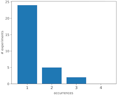
Figure 2. This figure represents the occurrence distribution of the best 10 configurations (out of a total of 256 experiments), that is, with the highest PSNR values, on the four input images.

In general, parameter initialization plays a crucial role in determining the final model performance and training time. This is evident by observing the range of PSNR-best obtained with the same image, same architecture, but different initialization methods from Table 1. In some cases the reason is a problem of convergence: the best PSNR has not been reached yet (3, 000 epochs). We define a number of epochs, risking not to reach the convergence, because we fit into a context of GreenAI where epochs are limited. On the other hand, setting an epoch number beforehand can be hazardous for those configurations that lead to semiconvergence. That is why in DIP-type models having a good Early Stopping criterion is crucial, a topic that is beyond the scope of this paper but will surely be included in the future.

TABLE 1

Table 1. The range of PSNR-best values for each image. The min PSNR and max PSNR represent the minimum and maximum PSNR-best among all experiments, respectively.

In Figures 3, 4 we show two different experiments; one among the trials with the best results (Figure 3) and one among the trials with the worst results (Figure 4). In detail, we analyzed for all 256 experiments the maximum PSNR reached for all four images. We then ranked among all PSNR maxima, for each of the four images, noting that one configuration emerged. This specific initialization, for which all learning curves performed well, shows early semi-convergence. On the other hand, analyzing the worst PSNR results, we noticed that one network gives bad performance for all images. What, in fact, can be noticed observing the images is that: on the left the PSNR grows very fast, reaching its peak before the 1, 000 epochs, which, associated with a good criterion of Early Stopping, can lead to a very good performance in few epochs, good result also in view of the GreenAI. While, observing the figure on the right, it can be seen that not even in 3, 000 epochs has reached a result comparable to the peak of the best initialization.

FIGURE 3

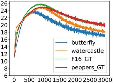
Figure 3. One of the experiments with the best results for all four images. This figure shows the PSNR curve. An example of the semiconvergence phenomenon.

FIGURE 4

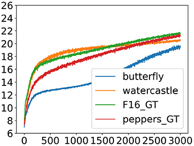
Figure 4. One of the experiments with the worst results for all four images. This figure shows the PSNR curve.

The experiment depicted in Figure 3 has the following initialization: the Convolutional weights with a Gaussian distribution (4: mean 0 and standard variation 0.001), the Convolutional biases with a Gaussian distribution (4: mean 0 and standard variation 0.001), the Batch Norm weights with a Gaussian distribution (3: mean 0 and standard variation 0.01), and the Batch Norm biases are set to zero (1). On the other hand, the experiment depicted in Figure 4 has the following initialization: the Convolutional weights with a Uniform distribution between [−1, 1] (2), the Convolutional biases with a uniform distribution between [0, 1] (1), the Batch Norm weights are set to one (1), and the Batch Norm biases are set to zero (1), very close to the initialization originally proposed in the paper [5]. In these two experiments we can observe that the first one reaches the maximum PSNR value, while the second one does not converge, not even in 3, 000 epochs. Both examples confirm what had already been observed in Table 2.

TABLE 2

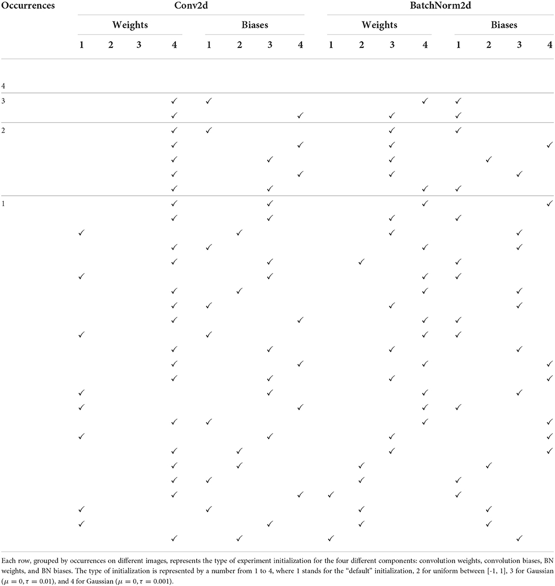
Table 2. This table shows the details of the experiments depicted in Figure 2.

Also in Figures 5, 6 we show two different experiments, but from another point of view. We decided to consider the best PSNR at 3, 000 epochs. In Figure 5 we can see the experiments with the best results and in Figure 6 the experiments with the worst results. In this case the observations that can be made are the mirror of the previous ones. In fact, the initializations that reach an early semi-convergence are the most penalized, starting soon to learn how to add noise to the image. While, the slower initializations, not being affected by semiconvergence, continue to grow, or at most stall up to 3, 000 epochs. However, this phenomenon is only evident by performing a large number of epochs, leading training times to be more than triple that of the best configuration.

FIGURE 5

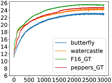
Figure 5. One of the experiments with the best results for all four images at the epoch 3, 000. This figure shows the PSNR curve.

FIGURE 6

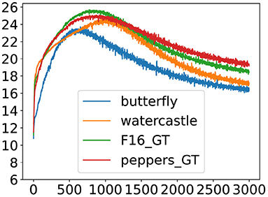
Figure 6. One of the experiments with the worst results for all four images at the epoch 3, 000. This figure shows the PSNR curve.

The experiment depicted in Figure 6 has the following initialization: the Convolutional weights with a Gaussian distribution (4. mean 0 and standard variation 0.001), the Convolutional biases are set with Uniform distribution between [0, 1] (1), the Batch Norm weights are set to one (1), and the Batch Norm biases are set with Uniform distribution between [-1, 1] (2). On the other hand, the experiment depicted in Figure 5 has the following initialization: the Convolutional weights with a Gaussian distribution (4: mean 0 and standard variation 0.001), the Convolutional biases with a Gaussian distribution (4: mean 0 and standard variation 0.001), the Batch Norm weights with a Gaussian distribution (4: mean 0 and standard variation 0.001), and the Batch Norm biases are set with Uniform distribution between [-1, 1] (2).

Another interesting result, which can be seen in Figures 7, 8, is the one concerning the convergence speed. In these four figures, we can see for the best 10 configurations mean and variance in statistical boxplot referred to the four different configuration types (x-axis) and epoch number (y-axis). For the best experiments, where we have seen that both the Convolutional weights and the Batch Norm weights are initialized with a Gaussian (Table 2), on average they are also the ones that reach convergence first, another time great for a context of GreenAI. From the point of view of the distribution of the weights at the end of the training, the only thing we can observe is that the weights distribute according to a Gaussian of zero mean, as known in the field of deep learning.

FIGURE 7

Figure 7. Initialization with respect to the convergence speed of the first top-K experiments (with K set to 10) with higher PSNR values for the butterfly image (A) and watercastle image (B).

FIGURE 8

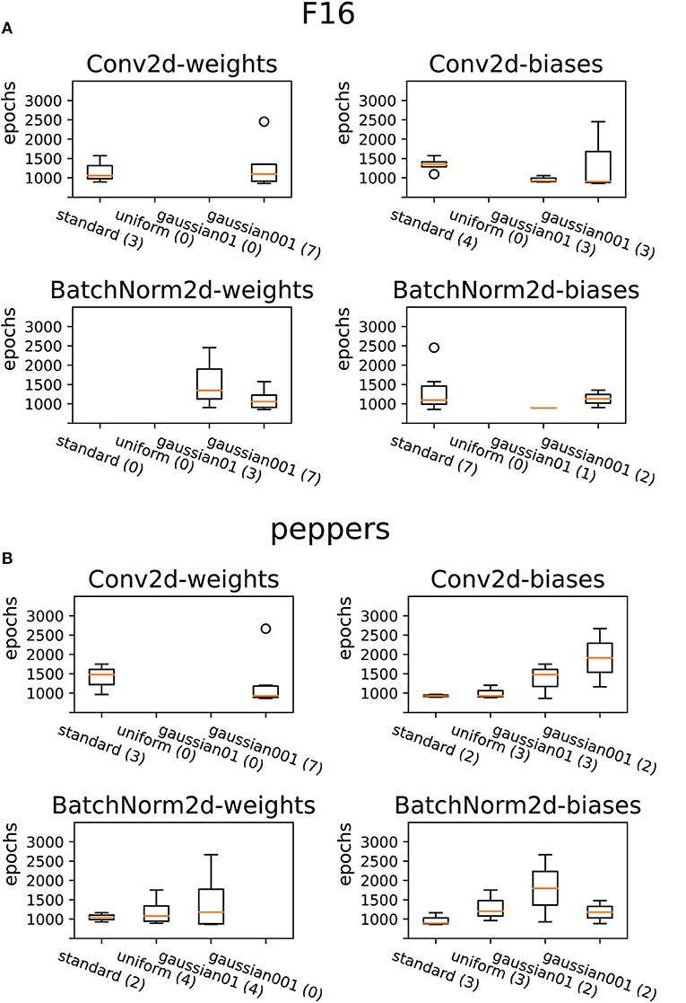
Figure 8. Initialization with respect to the convergence speed of the first top-K experiments (with K set to 10) with higher PSNR values for the F16 image (A) and peppers image (B).

4.2. Results on CT images

In the second part of experiments we will conduct some tests on images derived from biomedical CT examinations. As is well-known in the literature, this is a rather complex inverse problem due to several factors including: noise, limited angles image acquisition, and ill-conditioning of the matrix representing the tomographic transform. As an application of the DIP technique we will deal with noise removal on both CT images derived from a phantom, where we therefore know the ground-truth, and real biomedical images.

4.2.1. Experiments on the phantoms

In this section, we deal with the experiments conducted on the phantom. Experimentation was conducted on two sides for the purpose of approaching the problem of good biomedical image reconstruction. On the one hand, we tried the various experiments in different-resolution image contexts; to understand how resolution impacts the different initializations, and then shifted the focus, as with natural images, to the initializations that demonstrated good convergence behavior from the beginning. We chose to use the same phantom image, to which we added noise similar to the real tomographic image that we will use in the next section, amounting to about 5%. Thus, the idea is to take the image without noise and add Gaussian noise with zero mean and 0.05 variance. We considered two versions of the phantom image in the noisy version with different resolution, specifically we four specific initializations, in particular those configurations used in the study with the natural images. Similar to Figures 3–5 we looked for the best initialization in terms of convergence speed by validating the fact that configuration 4,431 (Figure 3) proves to be among the fastest, while configuration 4,442 (Figure 5) shows slower learning phase. In addition to this validation step, from Table 1 we identified another good initialization in configuration 4,141 (the Convolutional weights with a Gaussian distribution: mean 0 and standard variation 0.001, the Convolutional biases with a Uniform distribution, the Batch Norm weights with a Gaussian distribution: mean 0 and standard variation 0.001, and the Batch Norm biases are set to zero). It is important to note that with the phantom the phenomenon of semiconvergence is much less evident, suggesting that initializations that lead to fast improvement will be the best in terms of the final performance.

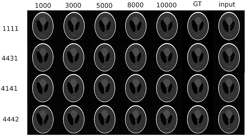
In Figure 9 we can see the phantom experiments in the resolution version 256 × 256. On the rows we observe, from top to bottom:

• the standard initialization proposed by the original paper [5],

• one of the best initializations for natural images, from the point of view of convergence speed (Figure 3),

• another good initialization found for natural images (second row of the Table 2),

• an initialization considered to be slow to converge for natural images (Figure 5).

FIGURE 9

Figure 9. Phantom experiments in the version 256 × 256.

On the columns, however, we can observe different stages of learning, indicated by the number of epochs. In the last column the noisy input image and in the penultimate column the ground-truth.

In Figure 10 we can see the same experiments for the phantom in the resolution version 512 × 512. A first observation that can be made is that image resolution does not impact behavior with respect to different initializations. A second observation, no less important, is that the fast or slow behavior of different initializations found with experiments on natural images can be transferred also for this image. This is very important, as it leads us to be able to use the information about initializations acquired with natural images for tomographic ones. The good or bad reconstruction of images is particularly evident in Figure 11 where we can see the zoom of some details of the reconstructed image. Indeed, we can well see from the details how the best initializations found for natural images (4,431, 4,141) are very good, in terms of PSNR. While we can observe how neither the original configuration of the original paper [5] nor the initialization that has been shown to be slow to converge for the natural images achieve at such good results.

FIGURE 10

Figure 10. Phantom experiments in the version 512 × 512.

FIGURE 11

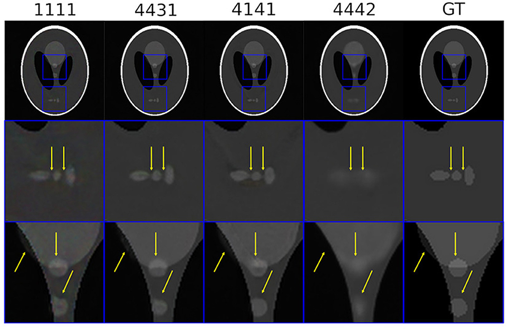
Figure 11. Some relevant details of the reconstruction of the phantom with different initializations.

4.2.2. Experiments on the real CT image

As a final experiment, an experiment was conducted on a real biomedical image. In this context, the analysis is complicated for several reasons: the noise percentage is not known, the ground-truth is not known for this reason there is no way to quantify the calculated PSNR against the real image, the image is much more complex and rich in detail, and it is not easy to make comparisons between reconstructions. For the percentage of noise in the biomedical image, a method known in the literature for estimating noise was used, arriving at a percentage of noise just under five percent. As for the qualitative assessment of the images, we relied on a literature paper [7] where the same image is already used, with specific details referenced to evaluate its accuracy.

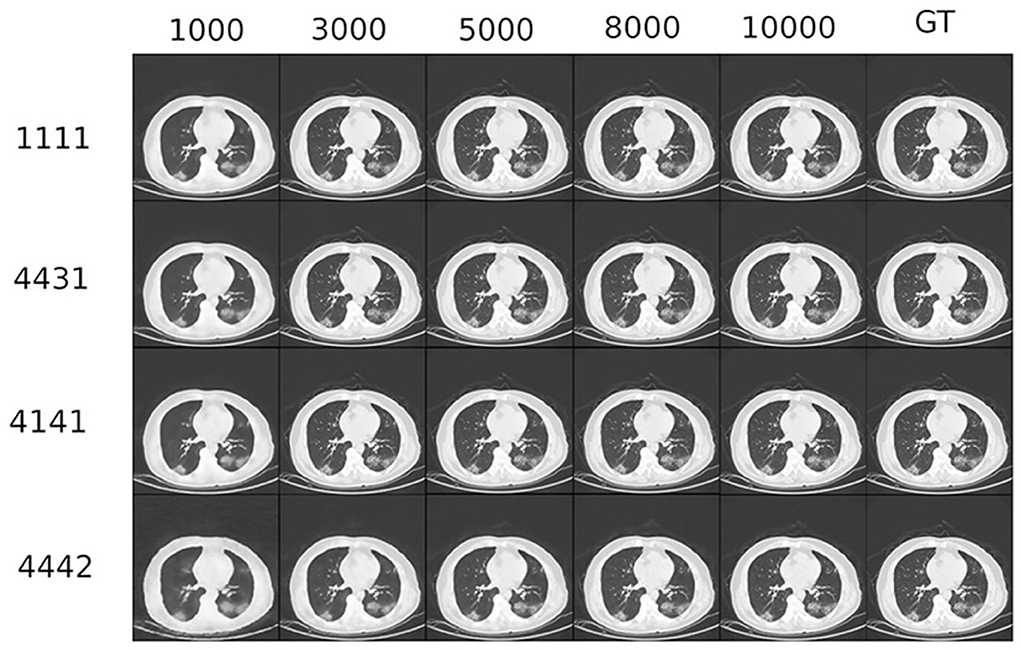
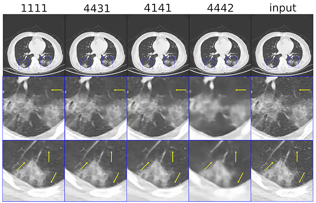
In Figure 12 we can see a table similar to the previous one for the phantom. What is observed, more in the Figure 13, is that even in the case of the tomographic image the (4,431 and 4,141) configurations show good initial behavior, while the (4,442) and the original paper initialization are shown to be slower in capturing image details.

FIGURE 12

Figure 12. Reconstruction in different epochs for CT real image.

FIGURE 13

Figure 13. Same details of the reconstruction CT image in different epochs for CT real image.

5. Conclusion and future works

As mentioned in the introduction, the main purpose of this work is to study how the choice of parameter initialization of an Autoencoder impacts performance and computation time. In particular, we analyzed a denoising problem approached with an unsupervised learning technique called DIP. This technique suffers from a phenomenon called semi-convergence, i.e., the Autoencoder initially learns to transform an image of pure noise into the assigned image, first incorporating the image characteristics, and then incorporating the noise as well. For the reasons just mentioned, the speed of convergence as a function of performance is essential. Recent works have attempted to study convergence speed from the point of view of the optimizer used, while others have tried to propose ad hoc Early Stopping techniques [25]. In this context, this paper aims to study the interpretability of this model through the various initializations in the literature. What we have observed, in conclusion, is that the different initializations of the weights have a great impact on the final performance, but in particular on the speed of convergence, which is fundamental in this context. On the other hand, we observed robustness concerning the analysis of different images, therefore the considerations made are portable to all images. In general, what we can conclude is that uniform initializations tend to bring slower results and thus require more training time. On the other hand, Gaussian initializations tend to be faster and, associated with Early Stopping techniques, can be considered better in a GreenAI context. Building on this initial work, the idea is to continue to analyze the weight distribution during the training phase, introduce pruning techniques and also examine the response with biomedical images, using, for example, Computed Tomography (CT).

Data availability statement

The original contributions presented in the study are included in the article/supplementary material, further inquiries can be directed to the corresponding author.

Author contributions

All authors listed have made a substantial, direct, and intellectual contribution to the work and approved it for publication.

Funding

This work was supported by the Gruppo Nazionale per il Calcolo Scientifico (GNCS-INdAM). The publication was created with the co-financing of the European Union-FSE-REACT-EU, PON Research and Innovation 2014–2020 DM1062/2021. The publication is co-financed from the project Artificial Intelligence-based Mathematical Models and Methods for low dose CT imaging, grant number 020143/21/FFP Prato Mission Oriented.

Conflict of interest

The authors declare that the research was conducted in the absence of any commercial or financial relationships that could be construed as a potential conflict of interest.

Publisher's note

All claims expressed in this article are solely those of the authors and do not necessarily represent those of their affiliated organizations, or those of the publisher, the editors and the reviewers. Any product that may be evaluated in this article, or claim that may be made by its manufacturer, is not guaranteed or endorsed by the publisher.

References

1. Buzug TM. Computed Tomography: From Photon Statistics to Modern Cone-Beam CT. Society Nuclear Medicine. Berlin; Heidelberg: Springer (2009).

Google Scholar

2. Goodfellow I, Pouget-Abadie J, Mirza M, Xu B, Warde-Farley D, Ozair S, et al. Generative adversarial nets. Proceedings of the 27th International Conference on Neural Information Processing Systems. Vol. 2 (2014). p. 2672–80.

Google Scholar

3. Kingma DP, Welling M. Auto-encoding variational Bayes. arXiv Preprint. (2013) arXiv:13126114. doi: 10.48550/arXiv.1312.6114

PubMed Abstract | CrossRef Full Text | Google Scholar

4. Dosovitskiy A, Springenberg JT, Tatarchenko M, Brox T. Learning to generate chairs, tables and cars with convolutional networks. IEEE Trans Pattern Anal Mach Intell. (2016) 39:692–705. doi: 10.1109/TPAMI.2016.2567384

PubMed Abstract | CrossRef Full Text | Google Scholar

5. Ulyanov D, Vedaldi A, Lempitsky V. Deep image prior. In: Proceedings of the IEEE Conference on Computer Vision and Pattern Recognition. Salt Lake City, UT (2018). p. 9446–54.

Google Scholar

6. Ledig C, Theis L, Huszár F, Caballero J, Cunningham A, Acosta A, et al. Photo-realistic single image super-resolution using a generative adversarial network. In: Proceedings of the IEEE Conference on Computer Vision and Pattern Recognition. Honolulu, HI (2017). p. 4681–90.

PubMed Abstract | Google Scholar

7. Cascarano P, Sebastiani A, Comes MC, Franchini G, Porta F. Combining weighted total variation and deep image prior for natural and medical image restoration via ADMM. In: 2021 21st International Conference on Computational Science and its Applications, (ICCSA). IEEE (2021). p. 39–46.

Google Scholar

8. Yan T, Wong PK, Ren H, Wang H, Wang J, Li Y. Automatic distinction between COVID-19 and common pneumonia using multi-scale convolutional neural network on chest CT scans. Chaos Solitons Fractals. (2020) 140:110153. doi: 10.1016/j.chaos.2020.110153

PubMed Abstract | CrossRef Full Text | Google Scholar

9. Bertsekas D. Nonlinear Programming. Belmont, MA: Athena Scientific (1999).

Google Scholar

10. Gould NIM, Lucidi S, Roma M, Toint P. Exploiting negative curvature directions in linesearch methods for unconstrained optimization. Optim Method Softw. (2000) 14:75–98. doi: 10.1080/10556780008805794

CrossRef Full Text | Google Scholar

11. Goodfellow I, Bengio Y, Courville A. Deep Learning. Cambridge, MA: The MIT Press (2016).

Google Scholar

12. Mishkin D, Matas J. All you need is a good initialization. arXiv Preprint. (2015) arXiv:151106422. doi: 10.48550/arXiv.1511.06422

CrossRef Full Text | Google Scholar

13. Aghajanyan A. Convolution aware initialization. arXiv Preprint. (2017) arXiv:170206295. doi: 10.48550/arXiv.1702.06295

CrossRef Full Text | Google Scholar

14. Arpit D, Campos V, Bengio Y. How to initialize your network? Robust initialization for weightnorm and Resnets. In: Advances in Neural Information Processing Systems 32 (NeurIPS 2019). Vancouver, BC (2019).

Google Scholar

15. Krähenbühl P, Doersch C, Donahue J, Darrell T. Data-dependent initializations of convolutional neural networks. arXiv Preprint. (2015) arXiv:151106856. doi: 10.48550/arXiv.1511.06856

CrossRef Full Text | Google Scholar

16. Krizhevsky A, Sutskever I, Hinton GE. Imagenet classification with deep convolutional neural networks. In: Advances in Neural Information Processing Systems 25 (NIPS 2012). Lake Tahoe, NE (2012).

Google Scholar

17. Glorot X, Bengio Y. Understanding the difficulty of training deep feedforward neural networks. In: Proceedings of the Thirteenth International Conference on Artificial Intelligence and Statistics. JMLR Workshop and Conference Proceedings. Sardinia (2010). p. 249–56.

Google Scholar

18. He K, Zhang X, Ren S, Sun J. Delving deep into rectifiers: Surpassing human-level performance on imagenet classification. In: Proceedings of the IEEE International Conference on Computer Vision. Santiago (2015). p. 1026–34.

Google Scholar

19. Ioffe S, Szegedy C. Batch normalization: accelerating deep network training by reducing internal covariate shift. In: International Conference on Machine Learning. PMLR, 2015. Lille (2015). p. 448–56.

Google Scholar

20. Sandjakoska L, Stojanovska F. How initialization is related to deep neural networks generalization capability: experimental study. In: 2020 55th International Scientific Conference on Information, Communication and Energy Systems and Technologies (ICEST). IEEE. Ni. (2020). p. 163–6.

Google Scholar

21. Xu B, Wang N, Chen T, Li M. Empirical evaluation of rectified activations in convolutional network. arXiv Preprint. (2015) arXiv:150500853. doi: 10.48550/arXiv.1505.00853

CrossRef Full Text | Google Scholar

22. Kingma DP, Ba J. Adam: a method for stochastic optimization. arXiv Preprint. (2014) arXiv:14126980. doi: 10.48550/arXiv.1412.6980

CrossRef Full Text | Google Scholar

23. Cascarano P, Franchini G, Porta F, Sebastiani A. On the first order optimization methods in deep image prior. Optimization Online. (2022). Available online at: https://optimization-online.org/?p=20038

PubMed Abstract | Google Scholar

24. Shepp LA, Logan BF. The Fourier reconstruction of a head section. IEEE Trans Nucl Sci. (1974) 21:21–43. doi: 10.1109/TNS.1974.6499235

CrossRef Full Text | Google Scholar

25. Wang H, Li T, Zhuang Z, Chen T, Liang H, Sun J. Early stopping for deep image prior. arXiv Preprint. (2021) arXiv:211206074. doi: 10.48550/arXiv.2112.06074

CrossRef Full Text | Google Scholar