Local stability analysis of two density-dependent semelparous species in two age classes

It is crucial to take into account the dynamics of the species while investigating how a species may survive in an environment. A species can be classified as either semelparous or iteroparous depending on how it reproduces. In this article, we present a model, which consists of two semelparous species by considering two age classes. We specifically discuss the effects of density-dependent in the interaction between the two semelparaous species and examine the equilibria of the system in the absence and presence of harvesting in the system. Then, the local stability of the equilibria is also investigated. A modified Leslie matrix population model with the addition of density-dependent in the equation is used. The model is analyzed in the presence and absence of competition between these species. We assume that density-dependent only occurred in the first age class of both species and that harvesting only occurred in the second age class of both species. Then, we assume that competition only occurs in the first age class in both species in the form of interspecific and intraspecific competition. This assumption is intended to simplify the complexity of the problem in the model. Our results show that there are three equilibria in the model without competition and four equilibria in the model with the competition. Hence, the presence of competition has influenced the number of equilibria. We also investigate the relation between the stability of the equilibria with the net reproduction rate of the system. Furthermore, we found the condition for the local stability of the co-existence equilibrium point, which is related to the degree of interspecific and intraspecific competition. This theory may be applied to investigate the dynamics of natural resources, whether in the absence of human exploitation and in the presence of various strategies in managing the exploitation of the resources, such as in fisheries industries.

1. Introduction

An ecosystem can be occupied by many species, which can be categorized either as semelparous species or iteroparous species. Semelparous species are species that reproduce only once in their life cycle. Some examples of semelparous species include cicada [1, 2], beetles [1], and salmon [3, 4]. On the other hand, iteroparous species are those that reproduce more than once during their life cycle. Examples of iteroparous species are easier to find than semelparous, including cows, cats, and many more. These species interact, such that the growth of one species is influenced by the growth of the other species. This is due to some limitations in ecosystems, like limited resources and bounded areas of the location. Because of this limitation, the environment may not meet the whole needs of the existing species. The population growth of the species is likely to be affected by their population. Similarly, species harvesting by humans for food may affects the growth of the species.

The dynamics of a population are very important to be studied with the aim of knowing the condition of the population in the future. This is because the growth of a population can lead to the increase, decrease, stability, or extinction of the population. There are several approaches used to describe the dynamics of the growth of a population in one species or multispecies in an ecosystem. One approach among several approaches is to model the growth of one species or multispecies based on population structure. Growth based on population structure focuses on dividing the overall population into smaller population structures. The population structure can be in the form of, among others, age class, stage of development, and population size.

Population structure allows us to study population growth more comprehensively, which cannot be described by other approaches. One example of a population based on a structure is a population based on age class. Population based on age class assumes that each age class has different characteristics including birth and survival rate. A population model based on the structure can be either continuous or discrete time. In recent years, the Leslie matrix model has been widely used as a discrete model of the population growth of a species based on age class. This model was introduced by Leslie [5]. The Leslie matrix model in the linear case form assumes that there are differences in birth rates and survival rates for each age class in population growth. The Leslie matrix model is linear when viewed from its growth graph. This model produces a growth graph that continues to rise, falls continuously, or is constant. Currently, the Leslie model has been widely developed on nonlinear models. The nonlinear Leslie matrix model is more realistic in representing real cases than the linear Leslie matrix model.

The development of the Leslie matrix model is not only limited to its linear and nonlinear forms, but it considers many aspects of the population. For example, the Leslie matrix model initially focused on single species cases, and furthermore, this model has also been developed for multispecies. Some of these studies observed growth models of species whose growth was influenced by density-dependence. Pennycuick et al. [6] focused on simulating the Leslie matrix model on single species and multispecies interactions. Travis et al. [7] conducted a study on Leslie's matrix model for two competing species and simulated the semelparous species. Kon [8] investigated two interacting semelparous species where one species has two age classes, and the other species have one age class. Kon [9] conducted a study on the Leslie matrix model of two semelparous species that have a predator-prey relationship and observed the coprime effect of the number of age classes of the two species. The number of age classes of two species is said to be mutually coprime if the two numbers (the number of classes of two species) have the greatest common factor equal to one. Then, Kon [10] examined the Leslie multispecies semelparous matrix model with an arbitrary number of species and an arbitrary number of interacting age classes. In addition, there are also several multispecies studies using other methods, both continuous time [11, 12], and discrete time [13].

Research on multispecies cases is very important because it is more realistic in describing real cases. However, the multispecies model is more complex than the single species model. This study invests in studying and modeling the population growth of multispecies. Our research focuses on the problem of multispecies population growth, which is influenced by dependence on population density and the effect of harvesting. Of course, this model can be used for both harvested and unharvested species, because if it is not harvested, the harvesting factor is zero. In addition, there are studies on the growth of single species that are affected by harvesting using the Leslie matrix model by Wikan [14]. Then, there is a study on harvesting cases with a different approach by Cooke et al. [15], Getz and Haight [16], Ganguli et al. [17], and Pratama et al. [18] as well as in the multispecies case of Hannesson et al. [19]. Other studies beside the effect of harvesting on the growth of the population, there are also some other studies related to obtaining the maximum sustainable yield, such as Supriatna and Possingham [20], Supriatna [21], Husniah and Supriatna [22], Supriatna and Husniah [23], Supriatna et al. [24], and Husniah et al. [25].

This study is limited to modeling two semelparous species with each species having two age classes. The model used in this paper is the Leslie matrix model for multispecies. In the model, it is assumed that there is a density-dependent influence on the growth of the species which only occurs in the first age class of the two species. In addition, growth for each species is also affected by harvesting which only occurs in the second age class. The model is analyzed under two headings, namely the multispecies model with no effect of interactions and the multispecies model with effect of interactions in the form of interspecific competition (competition between different species) and intraspecific competition (competition between the same species). Competition only occurs in the first age class in both species which is a response due to density-dependence.

This paper is presented as follows. Section 2 discusses the Leslie multispecies matrix model without interactions, determines the equilibrium point, and analyzes the stability of each equilibrium point. Section 3 discusses the Leslie multispecies matrix model with interactions in the form of interspecific competition and intraspecific competition, determines the equilibrium point of the model, and analyzes the stability of each equilibrium. Section 4 reports on the performance of the simulation, and Section 5 gives the concluding remarks.

2. Leslie matrix model of two semelparous species with density-dependent growth and harvesting without competition

This paper constructs and studies the growth dynamics of two semelparous species with each species having two age classes using the Leslie matrix for multispecies. The model with the number of two age classes can be applied to species that have a lifespan of 2 weeks, 2 months, 2 years, and two age stages can be children and adults, and so on. The model in this section is modified and constructed from the Travis et al. [7] and Wikan [14] models based on the assumptions and simplifications in this paper.

It is assumed that density-dependence only occurs in the first age class in each species. Then, harvesting only occurred in the second age class for both species. Both density-dependent and harvesting affect the population size of the second age class at time t + 1. In this case, the density-dependent factor uses the classical Beverton-Holt function whose effect is shown in Figure 1. The Beverton-Holt function is also used in research using the Leslie matrix by Wikan [14], but in this study, there is a simplification of the Beverton-Holt function. This model is given by the system of Equations (1) and is called Model A.

$\begin{array}{l}{x}_1(t+1)=f_{x_2}{x}_2(t),\end{array}$

$\begin{array}{ll}{x}_2(t+1)=\frac{s_{x_1}(1-h_{x_2})}{1+x_1(t)+y_1(t)}{x}_1(t),& (1)\end{array}$

$\begin{array}{l}{y}_1(t+1)=f_{y_2}{y}_2(t),\\ y_2(t+1)=\frac{s_{y_1}(1-h_{y_2})}{1+x_1(t)+y_1(t)}{y}_1(t),\end{array}$

where x_i(t) and y_i(t) represent the population densities of semelparous species x and y from the i-th age class (i = 1, 2) at time t, respectively. In this case f_x2, f_y2 > 0 represent the birth rate of species x and y in the second age class, respectively. Meanwhile, 0 < s_x1, s_y1 ≤ 1 each represents the survival rate of the first age to the second age class of species x and y. Finally, 0 < h_x2, h_y2 ≤ 1 are the harvesting rate in the second age class of species x and y, respectively. Based on the assumption, the density-dependent effect in Model A is modeled as $\frac{1}{1+x_1(t)+y_1(t)}$ where z in Figure 1 is x₁(t) + y₁(t). This is based on the assumption that density-dependence only occurs in the first age class in each species.

FIGURE 1

Figure 1. Density-dependent Beverton-Holt function.

The equilibrium point of model A can be done by making the left-hand side of model A dependent on time t so that the equilibria are given by the following system of equations:

$\begin{array}{l}{x}_1(t)=f_{x_2}{x}_2(t),\end{array}$

$\begin{array}{ll}{x}_2(t)=\frac{s_{x_1}(1-h_{x_2})}{1+x_1(t)+y_1(t)}{x}_1(t),& (2)\end{array}$

$\begin{array}{l}{y}_1(t)=f_{y_2}{y}_2(t),\\ y_2(t)=\frac{s_{y_1}(1-h_{y_2})}{1+x_1(t)+y_1(t)}{y}_1(t).\end{array}$

The system has the following equilibria:

i. The extinction equilibrium point

$\begin{array}{l}{E}_0=\left[\begin{array}{c}{x}_1\\ x_2\\ y_1\\ y_2\end{array}\right]=\left[\begin{array}{c}0\\ 0\\ 0\\ 0\end{array}\right],\end{array}$

implies, the extinction of both species.

ii. The extinction of the second species (species y) equilibrium point

$\begin{array}{l}{E}_x=\left[\begin{array}{c}{x}_1\\ x_2\\ y_1\\ y_2\end{array}\right]=\left[\begin{array}{c}(-f_{x_2}{s}_{x_1}(h_{x_2}-1)-1)\\ -\frac{(f_{x_2}{s}_{x_1}(h_{x_2}-1)+1)}{f_{x_2}}\\ 0\\ 0\end{array}\right]=\left[\begin{array}{c}{R}_x-1\\ -\frac{(-R_x+1)}{f_{x_2}}\\ 0\\ 0\end{array}\right],\end{array}$

with R_x = f_x2s_x1(1 − h_x2), where R_x represents the expected number of offspring per individual per lifetime when density-dependent effects are neglected on harvest-influenced growth of species x. Therefore, E_x exists if R_x > 1.

iii. The extinction of the first species (species x) equilibrium point

$\begin{array}{l}{E}_y=\left[\begin{array}{c}{x}_1\\ x_2\\ y_1\\ y_2\end{array}\right]=\left[\begin{array}{c}0\\ 0\\ (-f_{y_2}{s}_{y_1}(h_{y_2}-1)-1)\\ -\frac{(f_{y_2}{s}_{y_1}(h_{y_2}-1)+1)}{f_{y_2}}\end{array}\right]=\left[\begin{array}{c}0\\ 0\\ R_y-1\\ -\frac{(-R_y+1)}{f_{y_2}}\end{array}\right],\end{array}$

where R_y = f_y2s_y1(1 − h_y2). R_y represents the expected number of offspring per individual per lifetime when density-dependent effects are neglected on harvest-influenced growth of species y. Therefore, E_y exists if R_y > 1.

Based on the calculations, it is not interesting that the point of equilibrium at which both populations exist is not found in this model. Therefore, this model will be developed in Section 3 by adding interaction factors between species.

The following steps analyze the local stability of Model A. An equilibrium point is said to be asymptotically locally stable if the spectral radius of the Jacobian matrix at that equilibrium point is less than one. This criterion is difficult to apply to this model, so in this study, we use the M-Matrix method as done by Travis et al. [7]. The steps taken in the study of Travis et al. [7] to determine local stability asymptotically using the M-Matrix theory, include

i. Determining the Jacobian matrix from the equilibrium point. Suppose J(E) is an n × n matrix with E being the equilibrium point.

ii. Transformimg the J(E) matrix into a $G=I_n-SJ(E)S^{-1}$ matrix with I_n identity matrix of size n × n with S details can be seen in Travis et al. [7].

iii. Furthermore, the G matrix has a spectral radius of less than one if G is a M-matrix. A matrix is said to be M-Matrix if g_ij ≤ 0 for i ≠ j and if matrix G satisfies one of the five conditions, one of the conditions are that the principal minor of matrix G is positive [see for other conditions in Travis et al. [7]].

The locally stable asymptotic of each equilibrium point of Model A is presented in Theorem 1 below.

Theorem 1. For systems of Model A:

i. The equilibrium point E₀ is locally stable asymptotically if R_x < 1 and R_y < 1.

ii. The equilibrium point E_x is locally stable asymptotically if R_y < R_x and R_x > 1.

iii. The equilibrium point E_y is locally stable asymptotically if R_x < R_y and R_y > 1.

Proof. The local stability of each equilibrium point can be determined by linearizing the Model A. The Jacobian matrix of Model A becomes

$\begin{array}{ll}J(\left[x_1,x_2,y_1,y_2\right])=\left[\begin{array}{cccc}0& f_{x_2}& 0& 0\\ A_x(1+y_1)& 0& -A_x{x}_1& 0\\ 0& 0& 0& f_{y_2}\\ -A_y{y}_1& 0& A_y(1+x_1)& 0\end{array}\right],& (3)\end{array}$

where

$\begin{array}{l}{A}_x=\frac{s_{x_1}(1-h_{x_2})}{{(1+x_1+y_1)}^2},\\ A_y=\frac{s_{y_1}(1-h_{y_2})}{{(1+x_1+y_1)}^2}.\end{array}$

The next step is to substitute each equilibrium point into (3).

i. The Jacobian matrix for the equilibrium point E₀ is obtained as follows.

$\begin{array}{l}J(E_0)=\left[\begin{array}{cccc}0& f_{x_2}& 0& 0\\ s_{x_1}(1-h_{x_2})& 0& 0& 0\\ 0& 0& 0& f_{y_2}\\ 0& 0& s_{y_1}(1-h_{y_2})& 0\end{array}\right].\end{array}$

Based on the method used by Travis et al. [7], the Jacobian matrix J(E₀) will be transformed into a G matrix where $G=I_4-SJ(E_0)S^{-1}$. Because the value of J(E₀)₁₃, J(E₀)₁₄, J(E₀)₂₃, J(E₀)₂₄, J(E₀)₃₁, J(E₀)₃₂, J(E₀)₃₃, J(E₀)₃₄ ≤ 0 so that the chosen matrix S, i.e.,

$\begin{array}{l}S=\left[\begin{array}{cccc}1& 0& 0& 0\\ 0& 1& 0& 0\\ 0& 0& -1& 0\\ 0& 0& 0& -1\end{array}\right].\end{array}$

Therefore,

$\begin{array}{l}G=I_4-SJ(E_0)S^{-1}\\ =\left[\begin{array}{cccc}1& -f_{x_2}& 0& 0\\ -s_{x_1}(1-h_{x_2})& 1& 0& 0\\ 0& 0& 1& -f_{y_2}\\ 0& 0& -s_{y_1}(1-h_{y_2})& 1\end{array}\right].\end{array}$

Based on the defined parameters, the value of g_ij ≤ 0 for i ≠ j is fulfilled, where g_ij represents the elements of the G matrix in the i-th row of the j-th column so that G is called the M-matrix. Furthermore, the equilibrium point E₀ is locally stable asymptotically if all the minor principals of G are positive. Based on the calculation results obtained

$\begin{array}{l}\left|g_{11}\right|=1>0,\\ \left|\begin{array}{c}{g}_{11}{g}_{12}\\ g_{21}{g}_{22}\end{array}\right|=1+f_{x_2}{s}_{x_1}(h_{x_2}-1)\\ =1-R_x>0\Rightarrow R_x<1,\\ \left|\begin{array}{c}{g}_{11}{g}_{12}{g}_{13}\\ g_{21}{g}_{22}{g}_{23}\\ g_{31}{g}_{32}{g}_{33}\end{array}\right|=1+f_{x_2}{s}_{x_1}(h_{x_2}-1)\\ =1-R_x>0\Rightarrow R_x<1,\\ \left|\begin{array}{c}G\end{array}\right|=(1+f_{x_2}{s}_{x_1}(h_{x_2}-1))(1+f_{y_2}{s}_{y_1}(h_{y_2}\\ -1))=(1-R_x)(1-R_y)>0,\\ \Rightarrow R_x<1and{R}_y<1.\end{array}$

So, all the minor principals of G will be positive if R_x < 1 and R_y < 1. Therefore, the equilibrium point E₀ is locally stable asymptotically if R_x < 1 and R_y < 1.

ii. The Jacobian matrix for the equilibrium point E_x, i.e.,

$\begin{array}{l}J(E_x)=\left[\begin{array}{cccc}0& f_{x_2}& 0& 0\\ \frac{s_{x_1}(1-h_{x_2})}{R_x^2}& 0& -\frac{s_{x_1}(1-h_{x_2})(R_x-1)}{R_x^2}& 0\\ 0& 0& 0& f_{y_2}\\ 0& 0& -\frac{s_{y_1}(h_{y_2}-1)}{R_x}& 0\end{array}\right].\end{array}$

Next, the Jacobian matrix J(E_x) is transformed into a matrix $G=I_4-SJ(E_x)S^{-1}$. Because R_x > 1 and J(E_x)₁₃, J(E_x)₁₄, J(E_x)₂₃, J(E_x)₂₄, J(E_x)₃₁, J(E_x)₃₂, J(E_x)₃₃, and J(E_x)₃₄ ≤ 0 then,

$\begin{array}{l}S=\left[\begin{array}{cccc}1& 0& 0& 0\\ 0& 1& 0& 0\\ 0& 0& -1& 0\\ 0& 0& 0& -1\end{array}\right].\end{array}$

Furthermore,

$\begin{array}{l}G=\left[\begin{array}{cccc}1& -f_{x_2}& 0& 0\\ \frac{-s_{x_1}(1-h_{x_2})}{R_x^2}& 1& \frac{-s_{x_1}(1-h_{x_2})(R_x-1)}{R_x^2}& 0\\ 0& 0& 1& -f_{y_2}\\ 0& 0& \frac{-s_{y_1}(1-h_{y_2})}{R_x}& 1\end{array}\right].\end{array}$

Because R_x > 1 and the parameters are already defined, g_ij ≤ 0 is fulfilled for i ≠ j. The next step is to show that the principal minor of G is positive.Based on the calculation results obtained

$\begin{array}{l}\left|g_{11}\right|=1>0,\\ \left|\begin{array}{cc}{g}_{11}& g_{12}\\ g_{21}& g_{22}\end{array}\right|=\frac{1+f_{x_2}{s}_{x_1}(h_{x_2}-1)}{f_{x_2}{s}_{x_1}(h_{x_2}-1)}\\ =-\frac{1-R_x}{R_x}>0\Rightarrow R_x>1,\\ \left|\begin{array}{ccc}{g}_{11}& g_{12}& g_{13}\\ g_{21}& g_{22}& g_{23}\\ g_{31}& g_{32}& g_{33}\end{array}\right|=\frac{1+f_{x_2}{s}_{x_1}(h_{x_2}-1)}{f_{x_2}{s}_{x_1}(h_{x_2}-1)}\\ =-\frac{1-R_x}{R_x}>0\Rightarrow R_x>1,\\ \left|\begin{array}{c}G\end{array}\right|=\frac{(R_y-R_x)(1-R_x)}{R_x^2}>0\\ \Rightarrow R_x>1and{R}_y<R_x.\end{array}$

So, all minor principals of G will be positive if R_x > 1 and R_y < R_x. Therefore, the equilibrium point E_x is locally stable asymptotically if R_x > 1 and R_y < R_x.

iii. The Jacobian matrix for the equilibrium point E_y is

$\begin{array}{l}J(E_y)=\left[\begin{array}{cccc}0& f_{x_2}& 0& 0\\ \frac{s_{x_1}(1-h_{x_2})}{R_y}& 0& 0& 0\\ 0& 0& 0& f_{y_2}\\ \frac{-s_{y_1}(1-h_{y_2})(R_y-1)}{R_y^2}& 0& -\frac{s_{y_1}(h_{y_2}-1)}{R_y}& 0\end{array}\right].\end{array}$

Next, the Jacobian matrix J(E_y) is transformed into a matrix $G=I_4-SJ(E_y)S^{-1}$. Because R_y > 1 and J(E_y)₁₃, J(E_y)₁₄, J(E_y)₂₃, J(E_y)₂₄, J(E_y)₃₁, J(E_y)₃₂, J(E_y)₃₃, J(E_y)₃₄ ≤ 0 then,

$\begin{array}{l}S=\left[\begin{array}{cccc}1& 0& 0& 0\\ 0& 1& 0& 0\\ 0& 0& -1& 0\\ 0& 0& 0& -1\end{array}\right].\end{array}$

Furthermore,

$\begin{array}{l}G=\left[\begin{array}{cccc}1& -f_{x_2}& 0& 0\\ \frac{-s_{x_1}(1-h_{x_2})}{R_y}& 1& 0& 0\\ 0& 0& 1& -f_{y_2}\\ \frac{-s_{y_1}(1-h_{y_2})(R_y-1)}{R_y^2}& 0& \frac{-s_{y_1}(1-h_{y_2})}{R_y^2}& 1\end{array}\right].\end{array}$

Because R_y > 1 and the parameters are already defined, g_ij ≤ 0 is fulfilled for i ≠ j. The next step is to show that the principal minor of G is positive. Based on the calculation results obtained

$\begin{array}{l}\left|g_{11}\right|=1>0,\\ \left|\begin{array}{cc}{g}_{11}& g_{12}\\ g_{21}& g_{22}\end{array}\right|=\frac{-R_x+R_y}{R_y}>0=\frac{-R_x}{R_y}+1>0\\ \Rightarrow \frac{R_x}{R_y}<1\Rightarrow R_x<R_y,\\ \left|\begin{array}{ccc}{g}_{11}& g_{12}& g_{13}\\ g_{21}& g_{22}& g_{23}\\ g_{31}& g_{32}& g_{33}\end{array}\right|=\frac{-R_x+R_y}{R_y}>0=\frac{-R_x}{R_y}+1>0\\ \Rightarrow \frac{R_x}{R_y}<1\Rightarrow R_x<R_y,\\ \left|\begin{array}{c}G\end{array}\right|=-\frac{(R_y-R_x)(1-R_y)}{R_y^2}>0\\ \Rightarrow R_y>1and{R}_x<R_y.\end{array}$

So, all minor principals of G will be positive if R_y > 1 and R_x < R_y. Therefore, the equilibrium point E_y is locally stable asymptotically if R_y > 1 and R_x < R_y. This proof is complete.      ■

3. Leslie matrix model of two semelparous species with density-dependent growth and harvesting together with competition effect

Based on the previous model, there is no equilibrium point where the two species exist. In fact, in an ecosystem, it is expected that both species can survive. In this section, the previous model is improved upon. An assumption is added to the model that there are both intraspecific and interspecific competitions that occur only in the first age class as a density-dependent response. To simplify the problem, it is assumed that the level of competition between the first age class in species x and species y has the same value, i.e., a > 0. Then, the level of competition between the first age class in species y against species x and vice versa has the same value, i.e., b > 0. This problem is modeled in Equation (4) below and we call it Model B.

$\begin{array}{l}{x}_1(t+1)=f_{x_2}{x}_2(t),\end{array}$

$\begin{array}{ll}{x}_2(t+1)=\frac{s_{x_1}(1-h_{x_2})}{1+a{x}_1(t)+b{y}_1(t)}{x}_1(t),& (4)\end{array}$

$\begin{array}{l}{y}_1(t+1)=f_{y_2}{y}_2(t),\\ y_2(t+1)=\frac{s_{y_1}(1-h_{y_2})}{1+b{x}_1(t)+a{y}_1(t)}{y}_1(t).\end{array}$

Model B is an observed model from the model developed by Travis et al. [7] where in this model there is no effect of harvesting. Then, the model from Travis et al. [7] was modified and constructed based on the assumptions and simplifications in this research.

The equilibrium point of Model B can be determined by making the left-hand side of Model B dependent on the t-th time. The equilibrium solution of Model B is expressed in the following system of equations:

$\begin{array}{l}{x}_1(t)=f_{x_2}{x}_2(t),\end{array}$

$\begin{array}{ll}{x}_2(t)=\frac{s_{x_1}(1-h_{x_2})}{1+a{x}_1(t)+b{y}_1(t)}{x}_1(t),& (5)\end{array}$

$\begin{array}{l}{y}_1(t)=f_{y_2}{y}_2(t),\\ y_2(t)=\frac{s_{y_1}(1-h_{y_2})}{1+b{x}_1(t)+a{y}_1(t)}{y}_1(t).\end{array}$

By solving the Equation (5), we arrived at the following results:

i. The extinction equilibrium point is given as

$\begin{array}{l}{E}_0=\left[\begin{array}{c}{x}_1\\ x_2\\ y_1\\ y_2\end{array}\right]=\left[\begin{array}{c}0\\ 0\\ 0\\ 0\end{array}\right].\end{array}$

ii. The equilibrium point with species x exists is given as

$\begin{array}{l}{E}_x=\left[\begin{array}{c}{x}_1\\ x_2\\ y_1\\ y_2\end{array}\right]=\left[\begin{array}{c}-\frac{-R_x+1}{a}\\ -\frac{-R_x+1}{a{f}_{x_2}}\\ 0\\ 0\end{array}\right],\end{array}$

where R_x = f_x2s_x1(1 − h_x2). Therefore, E_x exists only if R_x > 1.

iii. The equilibrium point with species y exists is given as

$\begin{array}{l}{E}_y=\left[\begin{array}{c}{x}_1\\ x_2\\ y_1\\ y_2\end{array}\right]=\left[\begin{array}{c}0\\ 0\\ -\frac{-R_y+1}{a}\\ -\frac{-R_y+1}{a{f}_{y_2}}\end{array}\right],\end{array}$

where R_y = f_y2s_y1(1 − h_y2). Hence, E_y exists only if R_y > 1.

iv. The equilibrium point with both species exist given as

$\begin{array}{l}{E}_{xy}=\left[\begin{array}{c}{x}_1\\ x_2\\ y_1\\ y_2\end{array}\right]=\left[\begin{array}{c}-\frac{(a(-R_x+1)-b(-R_y+1))}{(a^2-b^2)}\\ -\frac{(a(-R_x+1)-b(-R_y+1))}{(a^2-b^2)f_{x_2}}\\ -\frac{(a(-R_y+1)-b(-R_x+1))}{(a^2-b^2)}\\ -\frac{(a(-R_y+1)-b(-R_x+1))}{(a^2-b^2)f_{y_2}}\end{array}\right].\end{array}$

There are two cases where the elements in E_xy are positive, namely

      Case 1 : $(a^2-b^2)>0,a(-R_x+1)-b(-R_y+1)<0$, and a(−R_y+1) − b(−R_x + 1) < 0.

      Case 2 : $(a^2-b^2)<0,a(-R_x+1)-b(-R_y+1)>0$, and a(−R_y + 1) − b(−R_x + 1) > 0.

Next, an asymptotically local stability analysis in Model A is performed. The steps taken to check the local stability in Model B are the same as in Model B. However, in Model B there are four equilibrium points that must be analyzed while in Model A there are only three equilibrium points due to the absence of a co-existence equilibrium point. The locally stable asymptotic for each equilibrium point of the model in Model B is presented in Theorem 2 below.

Theorem 2. For systems of Model B:

i. If R_x < 1 and R_y < 1, then the equilibrium point E₀ is locally stable asymptotically.

ii. If R_x > 1 and a(1 − R_y) > b(1 − R_x), then the equilibrium point E_x is locally stable asymptotically.

iii. If R_y > 1 and a(1 − R_x) > b(1 − R_y), then the equilibrium point E_y is locally stable asymptotically.

iv. If $(a^2-b^2)>0,a(1-R_x)<b(1-R_y)$, and a(1 − R_y) < b(1 − R_x), then the equilibrium point E_xy is locally stable asymptotically.

Proof: The Jacobian matrix of Model B is

$\begin{array}{ll}J(\left[x_1,x_2,y_1,y_2\right])=\left[\begin{array}{cccc}0& f_{x_2}& 0& 0\\ A_x(1+b{y}_1)& 0& -A_{x}b{x}_1& 0\\ 0& 0& 0& f_{y_2}\\ -A_{y}b{y}_1& 0& A_y(1+b{x}_1)& 0\end{array}\right],& (6)\end{array}$

where

$\begin{array}{l}{A}_x=\frac{s_{x_1}(1-h_{x_2}}{{(a{x}_1+b{y}_1+1)}^2},\\ A_y=\frac{s_{y_1}(1-h_{y_2}}{{(a{x}_1+b{y}_1+1)}^2}.\end{array}$

The next step is to substitute each equilibrium point into the Jacobian matrix in Equation (6).

i. The Jacobian matrix for the equilibrium point E₀, i.e.,

$\begin{array}{l}J(E_0)=\left[\begin{array}{cccc}0& f_{x_2}& 0& 0\\ s_{x_1}(1-h_{x_2})& 0& 0& 0\\ 0& 0& 0& f_{y_2}\\ 0& 0& s_{y_1}(1-h_{y_2})& 0\end{array}\right].\end{array}$

The same thing was done in determining the locally stable asymptotically of the Model A. First, the Jacobian matrix J(E₀) is transformed into the matrix $G=I_4-SJ(E_0)S^{-1}$. Because the value of J(E₀)₁₃, J(E₀)₁₄, J(E₀)₂₃, J(E₀)₂₄, J(E₀)₃₁, J(E₀)₃₂, J(E₀)₃₃, J(E₀)₃₄ ≤ 0 so that the chosen matrix S, i.e.,

$\begin{array}{l}S=\left[\begin{array}{cccc}1& 0& 0& 0\\ 0& 1& 0& 0\\ 0& 0& -1& 0\\ 0& 0& 0& -1\end{array}\right].\end{array}$

Furthermore,

$\begin{array}{l}G=\left[\begin{array}{cccc}1& -f_{x_2}& 0& 0\\ -s_{x_1}(1-h_{x_2})& 1& 0& 0\\ 0& 0& 1& -f_{y_2}\\ 0& 0& -s_{y_1}(1-h_{y_2})& 1\end{array}\right].\end{array}$

and g_ij ≤ 0 for i ≠ j. The next step is to show that the principal minor of G is positive. Based on the calculation results obtained

$\begin{array}{l}\left|g_{11}\right|=1>0,\\ \left|\begin{array}{cc}{g}_{11}& g_{12}\\ g_{21}& g_{22}\end{array}\right|=1-R_x>0\Rightarrow R_x<1,\\ \left|\begin{array}{ccc}{g}_{11}& g_{12}& g_{13}\\ g_{21}& g_{22}& g_{23}\\ g_{31}& g_{32}& g_{33}\end{array}\right|=1-R_x>0\Rightarrow R_x<1,\\ \left|\begin{array}{c}G\end{array}\right|=(1-R_x)(1-R_y)>0\\ \Rightarrow R_x<1and{R}_y<1.\end{array}$

So, all minor principals of G will be positive if R_y < 1 and R_x < 1. Therefore, the equilibrium point E₀ is locally stable asymptotically if R_x < 1 and R_y < 1.

ii. The Jacobian matrix for the equilibrium point E_x, i.e.,

$\begin{array}{l}J(E_x)=\left[\begin{array}{cccc}0& f_{x_2}& 0& 0\\ \frac{s_{x_1}(1-h_{x_2})}{R_x^2}& 0& -\frac{b{s}_{x_1}(1-h_{x_2})(R_x-1)}{a{R}_x^2}& 0\\ 0& 0& 0& f_{y_2}\\ 0& 0& -\frac{a{s}_{y_1}(h_{y_2}-1)}{(R_x-1)b+a}& 0\end{array}\right].\end{array}$

Next, the matrix J(E_x) is transformed into a matrix $G=I_4-SJ(E_x)S^{-1}$. Since R_x > 1, and the value of J(E_x)₁₃, J(E_x)₁₄, J(E_x)₂₃, J(E_x)₂₄, J(E_x)₃₁, J(E_x)₃₂, J(E_x)₃₃, J(E_x)₃₄ ≤ 0 so that the chosen matrix S, i.e.,

$\begin{array}{l}S=\left[\begin{array}{cccc}1& 0& 0& 0\\ 0& 1& 0& 0\\ 0& 0& -1& 0\\ 0& 0& 0& -1\end{array}\right].\end{array}$

Furthermore,

$\begin{array}{l}G=\left[\begin{array}{cccc}1& -f_{x_2}& 0& 0\\ -\frac{s_{x_1}(1-h_{x_2})}{R_x^2}& 1& -\frac{b{s}_{x_1}(1-h_{x_2})(R_x-1)}{a{R}_x^2}& 0\\ 0& 0& 1& -f_{y_2}\\ 0& 0& -\frac{a{s}_{y_1}(1-h_{y_2})}{(R_x-1)b+a}& 1\end{array}\right].\end{array}$

and g_ij ≤ 0 for i ≠ j. The next step is to show that the principal minor of G is positive. Based on the calculation results obtained

$\begin{array}{l}\left|g_{11}\right|=1>0,\\ \left|\begin{array}{cc}{g}_{11}& g_{12}\\ g_{21}& g_{22}\end{array}\right|=\frac{R_x-1}{R_x}>0\Rightarrow R_x>1,\\ \left|\begin{array}{ccc}{g}_{11}& g_{12}& g_{13}\\ g_{21}& g_{22}& g_{23}\\ g_{31}& g_{32}& g_{33}\end{array}\right|=\frac{R_x-1}{R_x}>0\Rightarrow R_x>1,\\ \left|\begin{array}{c}G\end{array}\right|=\frac{(R_x-1)(a(1-R_y)-b(1-R_x))}{R_x(a-b(1-R_x))}.\end{array}$

For |G|, R_x−1 > 0 and (a − b(1 − R_x)) > 0 because R_x > 1. Therefore, for |G| > 0, it must be (a(1 − R_y)−b(1 − R_x)) > 0 so that a(1 − R_y) > b(1 − R_x). Therefore, the equilibrium point E_x is locally stable asymptotically if R_x > 1 and a(1 − R_y) > b(1 − R_x).

iii. The Jacobian matrix for the equilibrium point E_y, i.e.,

$\begin{array}{l}J(E_0)=\left[\begin{array}{cccc}0& f_{x_2}& 0& 0\\ s_{x_1}(1-h_{x_2})& 0& 0& 0\\ 0& 0& 0& f_{y_2}\\ 0& 0& s_{y_1}(1-h_{y_2})& 0\end{array}\right].\end{array}$

Next, the matrix J(E_x) is transformed into a matrix $G=I_4-SJ(E_y)S^{-1}$. Since R_y > 1, the value of J(E_y)₁₃, J(E_y)₁₄, J(E_y)₂₃, J(E_y)₂₄, J(E_y)₃₁, J(E_y)₃₂, J(E_y)₃₃, and J(E_y)₃₄ ≤ 0 so that the chosen matrix S, i.e.,

$\begin{array}{l}S=\left[\begin{array}{cccc}1& 0& 0& 0\\ 0& 1& 0& 0\\ 0& 0& -1& 0\\ 0& 0& 0& -1\end{array}\right].\end{array}$

Furthermore,

$\begin{array}{l}G=\left[\begin{array}{cccc}1& -f_{x_2}& 0& 0\\ -s_{x_1}(1-h_{x_2})& 1& 0& 0\\ 0& 0& 1& -f_{y_2}\\ 0& 0& -s_{y_1}(1-h_{y_2})& 1\end{array}\right].\end{array}$

and g_ij ≤ 0 for i ≠ j. The next step is to show that the principal minor of G is positive. Based on the calculation results obtained

$\begin{array}{l}\left|g_{11}\right|=1>0,\\ \left|\begin{array}{cc}{g}_{11}& g_{12}\\ g_{21}& g_{22}\end{array}\right|=\frac{(a(1-R_x)-b(1-R_y))}{a-b(1-R_y)},\\ \left|\begin{array}{ccc}{g}_{11}& g_{12}& g_{13}\\ g_{21}& g_{22}& g_{23}\\ g_{31}& g_{32}& g_{33}\end{array}\right|=\frac{(a(1-R_x)-b(1-R_y))}{a-b(1-R_y)},\\ \left|\begin{array}{c}G\end{array}\right|=-\frac{(1-R_y)(a(1-R_x)-b(1-R_y))}{R_y(a-b(1-R_y))}.\end{array}$

Since R_y > 1, consequently, (1 − R_y) < 0 and (a − b(1 − R_y)) > 0. Therefore, for all minor principals to be positive, it must be (a(1 − R_x)−b(1 − R_y)) > 0 so that a(1 − R_x) > b(1 − R_y). Thus, the equilibrium point E_y is locally stable asymptotically if R_y > 1 and a(1 − R_x) > b(1 − R_y).

iv. The Jacobian matrix for the equilibrium point E_xy, i.e.,

$\begin{array}{l}J(E_{xy})=\left[\begin{array}{cccc}0& f_{x_2}& 0& 0\\ A_1& 0& A_2& 0\\ 0& 0& 0& f_{y_2}\\ B_1& 0& B_2& 0\end{array}\right],\end{array}$

where

$\begin{array}{l}{A}_1=\frac{b^2{R}_x+a(-a+(1-R_y)b)}{-R_x{f}_{x_2}(a^2-b^2)},\\ A_2=\frac{b(a(1-R_x)-b(1-R_y))}{R_x{f}_{x_2}(a^2-b^2)},\\ B_1=\frac{b(a(1-R_y)-b(1-R_x))}{R_y{f}_{y_2}(a^2-b^2)},\\ B_2=\frac{b^2{R}_y+a(-a+(1-R_x)b)}{-R_y{f}_{y_2}(a^2-b^2)}.\end{array}$

Next, the matrix J(E_xy) is transformed into a matrix $G=I_4-SJ(E_{xy})S^{-1}$. Because between a(1 − R_x)−b(1 − R_y) and a(1 − R_y)−b(1 − R_x) to a²−b² have different signs which is a condition where the equilibrium point E_xy exists. As a result, A₂ and B₂ are negative. Therefore, the value of J(E_xy)₁₃, J(E_xy)₁₄, J(E_xy)₂₃, J(E_xy)₂₄, J(E_xy)₃₁, J(E_xy)₃₂, J(E_xy)₃₃, and J(E_xy)₃₄ ≤ 0 so that the chosen matrix S, i.e.,

$\begin{array}{l}S=\left[\begin{array}{cccc}1& 0& 0& 0\\ 0& 1& 0& 0\\ 0& 0& -1& 0\\ 0& 0& 0& -1\end{array}\right].\end{array}$

Furthermore,

$\begin{array}{l}G=\left[\begin{array}{cccc}1& -f_{x_2}& 0& 0\\ A_1& 1& A_2& 0\\ 0& 0& 1& -f_{y_2}\\ B_1& 0& B_2& 1\end{array}\right].\end{array}$

In addition, g_ij ≤ 0 for i ≠ j. The next step is to show that the principal minor of G is positive. Based on the calculation results obtained

$\begin{array}{l}J(E_y)=\left[\begin{array}{cccc}0& f_{x_2}& 0& 0\\ \frac{a{s}_{x_1}(1-h_{x_2})}{(R_y-1)b+a}& 0& 0& 0\\ 0& 0& 0& f_{y_2}\\ -\frac{b{s}_{y_1}(1-h_{y_2})(R_y-1)}{a{R}_y^2}& 0& -\frac{s_{y_1}(h_{y_2}-1)}{(R_y^2}& 0\end{array}\right].\end{array}$

The results above show that only |g₁₁| is positive, so there are three minor principals that must be determined to be positive. The three minor principals will be positive if $(a^2-b^2)>0,a(-R_x+1)-b(-R_y+1)<0$, and a(−R_y+1)−b(−R_x+1) < 0. Thus, the equilibrium point E_xy is locally stable asymptotically if $a(a^2-b^2)>0,a(-R_x+1)-b(-R_y+1)<0$, and a(−R_y+1)−b(−R_x+1) < 0. The proof is complete.      ■

4. Numerical simulations

In the previous sections, analytical analyses of the existence and locally stable asymptotically of each equilibrium point have been carried out in Models A and B. This section presents some numerical simulation results with the aim of providing numerical proof of Theorems 1 and 2 of this study. The graphical results of the numerical proof are presented in Figures 2–8. In this study, the specific species in question is not determined. For this reason, some of the parameter values used in the numerical simulation are hypothetical parameters. In this case, simulations are performed on both models and each model will be divided into several cases based on the stability conditions of each equilibrium point.

FIGURE 2

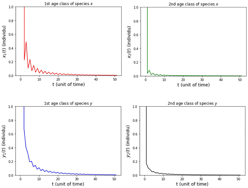
Figure 2. Population growth of each age class from case (i) Model A.

In the numerical simulation of Model A, the simulation is divided into three cases. It is assumed for all the cases that the parameter values are s_x1 = 0.3 and s_y1 = 0.3. Both of these parameters were obtained in the research of Travis et al. [7]. The other parameters for each case in the numerical simulation of Model A 275 is presented as follows:

(i) f_x2 = 6, f_y2 = 4, h_x2 = 1/2, and h_y2 = 1/4 so that R_x = 0.89 and R_y = 0.89.

(ii) f_x2 = 20, 000, f_y2 = 500, h_x2 = 0.001, and h_y2 = 1/4 so that R_x = 5, 994 and R_y = 22.5.

(iii) f_x2 = 500, f_y2 = 20, 000, h_x2 = 0.001, and h_y2 = 1/4 so that R_x = 149.85 and R_y = 4500.

The parameter value for the birth rate of 20,000 follows the value of the birth rate parameter in the study of Travis et al. [7]. All parameter values are measured per unit of time and the total population is calculated per individual.

The results of simulation on Model A for cases (i)-(iii) are presented in Figures 2–4. Figure 2 shows the case (i), in which R_x < 1 and R_y < 1, resulting in the stability of the system toward the equilibrium point E₀. Figure 3 shows case (ii), in which R_x > 1 and R_x > R_y, resulting in the stability of the system toward the equilibrium point $E_x={\left[5993,0.3,0,0\right]}^T$, i.e., species x exists. Figure 4 shows case (iii), in which R_y > 1 and R_y > R_x, resulting in the stability of the system toward the equilibrium point $E_y={\left[0,0,4499,0.22\right]}^T$ i.e., species y exists.

FIGURE 3

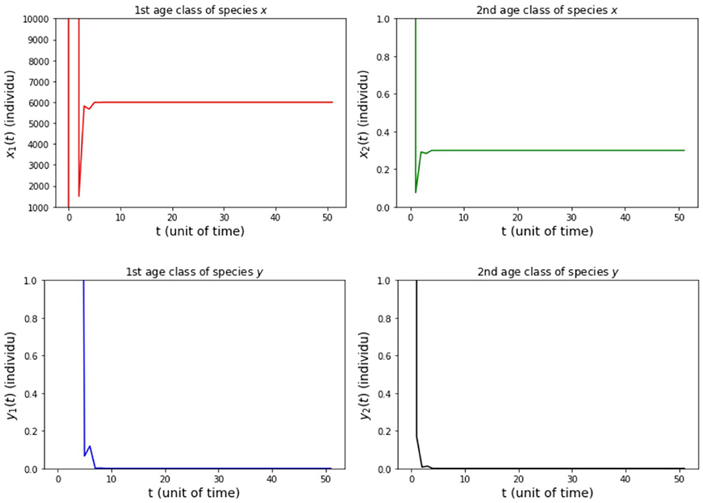
Figure 3. Population growth of each age class from case (ii) Model A.

FIGURE 4

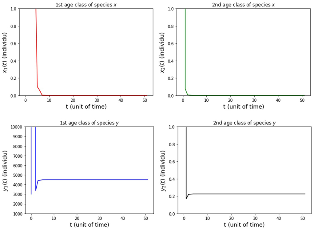
Figure 4. Population growth of each age class from case (iii) Model A.

In the numerical simulation of Model B, the simulation is divided into four cases. It is assumed that the survival rate of Model B is the same as the survival rate of Model A. It is also assumed that the level of intraspecific competition is a = 0.05 and the level of interspecific competition is b = 0.01. The values of a and b indicate that a²−b² > 0. This choice was made to minimize the simulations carried out. Then, we assume the value of the parameters h_x2 = 1/2 and h_y2 = 1/4 for all cases of Model B. The other parameters for each case in the numerical simulation of Model B are presented as follows:

(i) f_x2 = 6 and f_y2 = 4 so that R_x = 0.89 and R_y = 0.89.

(ii) f_x2= 20,000 and f_y2 = 500 so that R_x= 3,000 and R_y = 112.5.

(iii) f_x2 = 500 and f_y2= 20,000 so that R_x = 75 and R_y= 4,500.

(iv) f_x2= 20,000 and f_y2= 10,000 so that R_x= 3,000 and R_y= 2,250.

The results of the numerical simulation on Model B are shown in Figures 5–8. Figure 5 shows case (i), in which R_x < 1 and R_y < 1, resulting in the stability of the system toward the equilibrium point E₀. Figure 6 shows the case (ii), in which R_x > 1 and a(1 − R_y) > b(1 − R_x), resulting in the stability of the system toward the equilibrium point $E_x={\left[59980,3,0,0\right]}^T$ where species x exists. Figure 7 shows case (iii), in which R_y > 1 and a(1 − R_x) > b(1 − R_y), resulting in the stability of the system toward the equilibrium point $E_y={\left[0,0,89980,4.495\right]}^T$. Figure 8 shows case (iv), in which a > b, a(1 − R_x) < b(1 − R_y), and a(1 − R_y) < b(1 − R_x), resulting in the stability of the system toward the equilibrium point $E_{xy}={\left[53108.33,2.65,34358.33,3.43\right]}^T$.

FIGURE 5

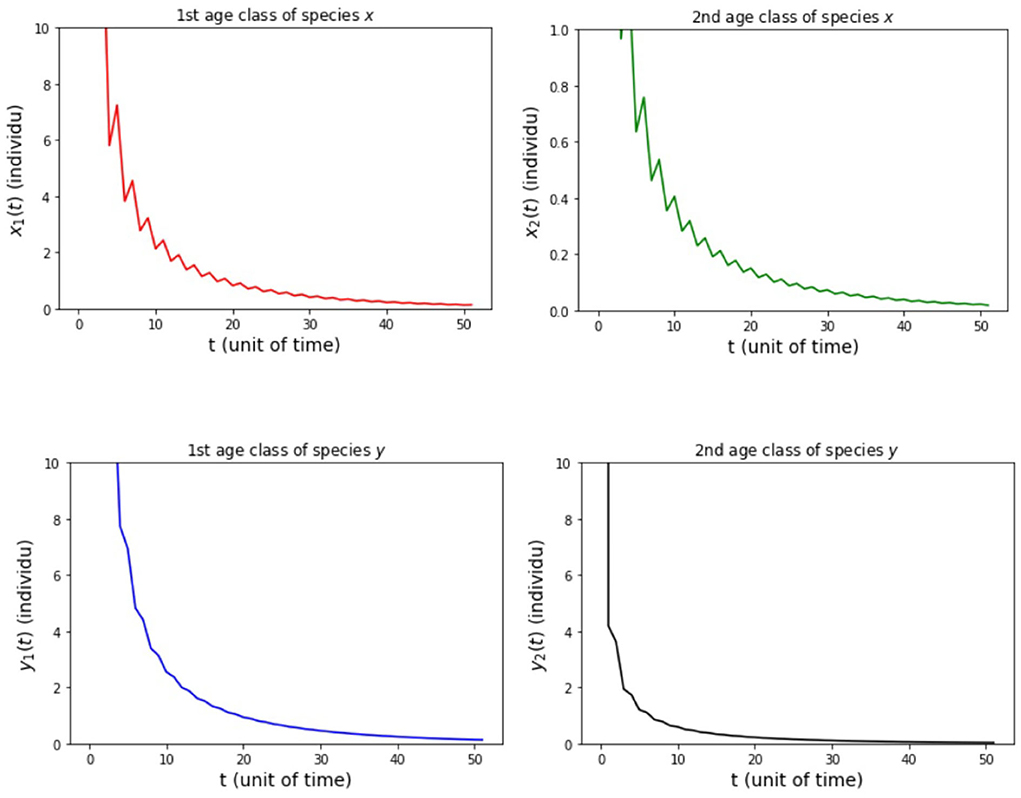
Figure 5. Population growth of each age class from case (i) Model B.

FIGURE 6

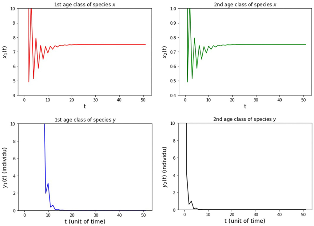
Figure 6. Population growth of each age class from case (ii) Model B.

FIGURE 7

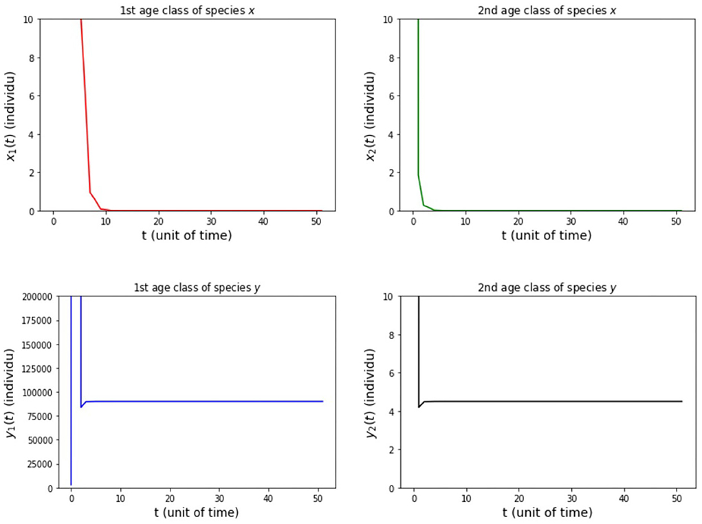
Figure 7. Population growth of each age class from case (iii) Model B.

FIGURE 8

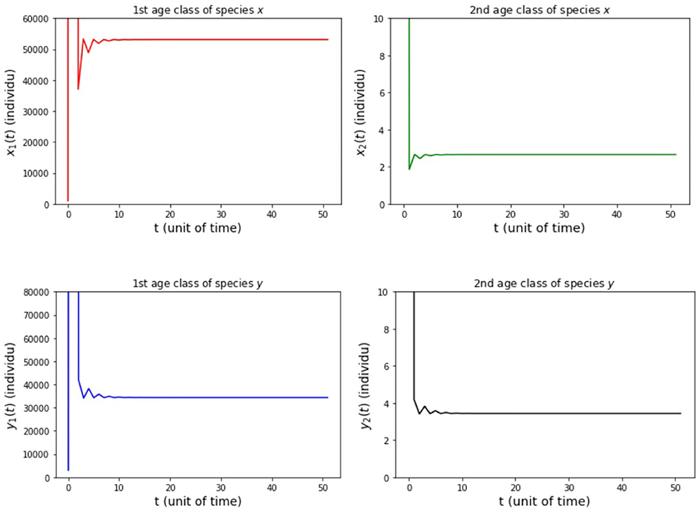
Figure 8. Population growth of each age class from case (iv) Model B.

5. Discussion

The research presented in this paper is an extension of the model carried out by Pennycuick et al. [6], Travis et al. [7], and Kon [8–10]. In these studies, the effect of harvesting on species growth which is influenced by density-dependence and competition has not been studied. These influences on the growth of species can occur in an ecosystem as in the case study on fish conducted by Travis et al. [7] in his research. This extended model can also be applied to the species growth model without the effect of harvesting with the value of the harvesting level equal to zero.

In this paper, we find several results in the comparison of the models we developed, namely Model A and Model B. In Model A, there is no co-existence equilibrium point between the two semelparous species in the same ecosystem, but this point has only been found in Model B. It can be concluded that the competition affects the existence of a co-existence equilibrium point in the density-dependent growth of the two species. In addition, the local stability in Model A and Model B is also explored. The asymptotically local stability of Model A depends on the condition of the inherent net reproduction number of species x (R_x) and the inherent net reproduction number of species y (R_y). Then, the asymptotically local stability of Model B depends on the values of R_x, R_y, the level of intraspecific competition (a), and the level of interspecific competition (b).

6. Conclusion

In this paper, population growth models of two semelparous species have been studied where growth is influenced by density-dependent and harvesting. The models are analyzed with no competition as in Model A and with competition as in Model B. Based on the results, the factors that influence both the existence of the equilibrium point and its locally stable asymptotically are the values of a, b, R_x (net reproductive value of species x with harvesting effect), and R_y (net reproductive value of species y with harvesting effect). Overall, both the equilibrium points and their local stability are determined by the parameters R_x and R_y, which implies that harvesting is very influential. Besides, in Model A, there is no equilibrium point where both species exist. Therefore, Model A was developed into Model B and it turned out that adding the factors of intraspecific competition (a) and interspecific competition (b) affect the equilibrium point where the two species require that a ≠ b. Then, the values of parameters a and b also play a role in determining the local stability conditions from the equilibrium point where both species exist. Observations on multispecies growth are closer to the real problem than single species growth. However, the multispecies growth model is difficult to work with. Hence, there is a simplification of the particular model currently being investigated. This study still focuses on the simple problem of the growth of two semelparous species that are affected by density-dependent, competition, and harvesting. Future work that can be developed from this research include research on the number of any age class, the number of any species, global stability problems, bifurcation problems, and many more.

Data availability statement

The original contributions presented in the study are included in the article/supplementary material, further inquiries can be directed to the corresponding author/s.

Author contributions

AS: design and supervise the research. AH: develop and analyze the models. EC: conducting literature review. All authors contributed to the article and approved the submitted version.

Funding

The authors would like to thank the Indonesia Government who provided fund for the APC of the publication in this journal through the scheme of Penelitian Tesis Magister (PTM)-2022 with contract number 1318/UN6.3.1/PT.00/2022.

Acknowledgments

The work is part of the research during the M.Sc. candidature of AH. AH would like to thank for the tuition fee during the candidature covered by ALG-Unpad Research Grant for the year 2020-2021 with contract number 1959/UN6.3.1/PT.00/2021.

Conflict of interest

The authors declare that the research was conducted in the absence of any commercial or financial relationships that could be construed as a potential conflict of interest.

Publisher's note

All claims expressed in this article are solely those of the authors and do not necessarily represent those of their affiliated organizations, or those of the publisher, the editors and the reviewers. Any product that may be evaluated in this article, or claim that may be made by its manufacturer, is not guaranteed or endorsed by the publisher.

References

1. Chow Y, Kon R. Global dynamics of a special class of nonlinear semelparous Leslie matrix models. J Diff Equat Appl. (2020) 26:1777288. doi: 10.1080/10236198.2020.1777288

CrossRef Full Text | Google Scholar

2. Diekmann O, Planqué R. The winner takes it all: how semelparous insects can become periodical. J Math Biol. (2020) 80:283–301. doi: 10.1007/s00285-019-01362-3

PubMed Abstract | CrossRef Full Text | Google Scholar

3. Diekmann O, Davydova N, Van Gils S. On a boom and bust year class cycle. J Diff Equat Appl. (2005) 11:327–35. doi: 10.1080/10236190412331335409

CrossRef Full Text | Google Scholar

4. Davydova NV, Diekmann O, Gils SAV. Year class coexistence or competitive exclusion for strict biennials? J Math Biol. (2003) 46:95–131. doi: 10.1007/s00285-002-0167-5

PubMed Abstract | CrossRef Full Text | Google Scholar

5. Leslie PH. On the use of matrices in certain population mathematics. Biometrika. (1945) 33:183. doi: 10.1093/biomet/33.3.183

PubMed Abstract | CrossRef Full Text | Google Scholar

6. Pennycuick CJ, Compton RM, Beckingham L. A computer model for simulating the growth of a population, or of two interacting populations. J Theor Biol. (1968) 18:316–29. doi: 10.1016/0022-5193(68)90081-7

PubMed Abstract | CrossRef Full Text | Google Scholar

7. Travis CC, Post WM, DeAngelis DL, Perkowski J. Analysis of compensatory Leslie matrix models for competing species. Theor Popul Biol. (1980) 18:16–30. doi: 10.1016/0040-5809(80)90037-4

PubMed Abstract | CrossRef Full Text | Google Scholar

8. Kon R. Age-structured Lotka-Volterra equations for multiple semelparous populations. SIAM J Appl Math. (2011) 21:694–713. doi: 10.1137/100794262

CrossRef Full Text | Google Scholar

9. Kon R. Permanence induced by life-cycle resonances: the periodical cicada problem. J Biol Dyn. (2012) 6:855–90. doi: 10.1080/17513758.2011.594098

PubMed Abstract | CrossRef Full Text | Google Scholar

10. Kon R. Stable bifurcations in multi-species semelparous population models. In: Elaydi SMHHY, Potzsche C, editor. Springer Proceedings in Mathematics and Statistics. Vol. 212. New York, NY: Springer New York LLC (2017). p. 3–25.

11. Beay LK, Suryanto A, Suryanto A, Suryanto A. Stability of a stage-structure Rosenzweig-MacArthur model incorporating Holling type-II functional response. In: IOP Conference Series: Materials Science and Engineering. (2019). Available online at: https://iopscience.iop.org/article/10.1088/1757-899X/546/5/052017

12. Savadogo A, Sangaré B, Ouedraogo H. A mathematical analysis of Hopf-bifurcation in a prey-predator model with nonlinear functional response. Adv Diff Equat. (2021) 2021:275. doi: 10.1186/s13662-021-03437-2

CrossRef Full Text | Google Scholar

13. Fang L, N'gbo N, Xia Y. Almost periodic solutions of a discrete Lotka-Volterra model via exponential dichotomy theory. Am Inst Math Sci. (2022) 7:3788–801. doi: 10.3934/math.2022210

CrossRef Full Text | Google Scholar

14. Wikan A. Dynamical consequences of harvest in discrete age-structured population models. J Math Biol. (2004) 49:35–55. doi: 10.1007/s00285-003-0251-5

PubMed Abstract | CrossRef Full Text | Google Scholar

15. Cooke KL, Elderkin R, Witten M. Harvesting procedures with management policy in iterative density-dependent population models. Nat Resour Model. (1988) 2:383–420. doi: 10.1111/j.1939-7445.1988.tb00065.x

CrossRef Full Text | Google Scholar

16. Haight RG, Getz WM. Population Harvesting: Demographic Models of Fish, Forest, and Animal Resources. Princeton, NJ: Princeton University Press (1989).

17. Ganguli C, Kar TK, Mondal PK. Optimal harvesting of a prey-predator model with variable carrying capacity. Int J Biomath. (2017) 10:17500693. doi: 10.1142/S1793524517500693

PubMed Abstract | CrossRef Full Text | Google Scholar

18. Pratama RA, Ruslau MFV, Nurhayati. Global analysis of stage structure two predators two prey systems under harvesting effect for mature predators. In: Journal of Physics: Conference Series. Vol. 1899. IOP Publishing Ltd (2021). Available online at: https://iopscience.iop.org/article/10.1088/1757-899X/546/5/052017

19. Hannesson R, Flåten O, Hannesson R, Flaten O. The economics of multispecies harvesting. Scand J Econ. (1989) 91:340091. doi: 10.2307/3440091

CrossRef Full Text | Google Scholar

20. Supriatna AK, Possingham HP. Harvesting a two-patch predator-prey metapopulation. Nat Resour Model. (1999) 12:481–98. doi: 10.1111/j.1939-7445.1999.tb00023.x

CrossRef Full Text | Google Scholar

21. Supriatna AK. Maximum sustainable yield for marine metapopulation governed by coupled generalised logistic equations. J Sustain Sci Manag. (2012) 7:201–6. Available online at: https://jssm.umt.edu.my/files/2012/11/13.pdf

22. Husniah H, Supriatna AK. Marine biological metapopulation with coupled logistic growth functions: the MSY and quasi MSY. In: AIP Conference Proceedings. Makassar (2014). Available online at: https://aip.scitation.org/doi/10.1063/1.4866532

23. Supriatna AK, Husniah H. Sustainable harvesting strategy for natural resources having a coupled Gompertz production function. In: Interdisciplinary Behavior and Social Sciences - Proceedings of the 3rd International Congress on Interdisciplinary Behavior and Social Sciences, ICIBSoS 2014. Bali (2015). Available online at: https://www.taylorfrancis.com/chapters/edit/10.1201/b18146-19/sustainable-harvesting-strategy-natural-resources-coupled-gompertz-production-function-supriatna-husniah

24. Supriatna AK, Ramadhan AP, Husniah H. A decision support system for estimating growth parameters of commercial fish stock in fisheries industries. Procedia Comput Sci. (2015) 59:331–9. doi: 10.1016/j.procs.2015.07.575

CrossRef Full Text | Google Scholar

25. Husniah H, Anggriani N, Supriatna AK. System dynamics approach in managing complex biological resources. ARPN J Eng Appl Sci. (2015) 10. Available online at: https://www.arpnjournals.com/jeas/research_papers/rp_2015/jeas_0315_1650.pdf