 Oralia Nolasco-Jáuregui
 L. A. Quezada-Téllez2
95% of researchers rate our articles as excellent or good
Learn more about the work of our research integrity team to safeguard the quality of each article we publish.
Find out more
ORIGINAL RESEARCH article
Front. Appl. Math. Stat. , 02 June 2022
Sec. Statistics and Probability
Volume 8 - 2022 | https://doi.org/10.3389/fams.2022.848898
This article is part of the Research Topic Statistical Data Science - Theory and Applications in Analyzing Omics Data View all 8 articles
In December 2019, the COVID-19 pandemic began, which has claimed the lives of millions of people around the world. This article presents a regional analysis of COVID-19 in Mexico. Due to comorbidities in Mexican society, this new pandemic implies a higher risk for the population. The study period runs from 12 April to 5 October 2020 761,665. This article proposes a unique methodology of random matrix theory in the moments of a probability measure that appears as the limit of the empirical spectral distribution by Wigner's semicircle law. The graphical presentation of the results is done with Machine Learning methods in the SuperHeat maps. With this, it was possible to analyze the behavior of patients who tested positive for COVID-19 and their comorbidities, with the conclusion that the most sensitive comorbidities in hospitalized patients are the following three: COPD, Other Diseases, and Renal Diseases.
Throughout its history, humanity has faced several pandemics in which millions of people lost their lives around the world. The recent epidemics of SARS-CoV and MERS-CoV stand out [1]. In December 2019, in the city of Wuhan China, a series of cases were reported that met the criteria for pneumonia with severe characteristics. Local health authorities noted an epidemiological relationship in the patients with a wholesale seafood market, where wild animals were also sold [2].
By 31 December, the Chinese Center for Disease Control and Prevention was notified and began an epidemiological investigation. As a first security measure, the seafood market was closed to the public on 1 January 2020. On 9 January, the Chinese government reported the discovery of the new coronavirus, and on 12 January, they released their genomic sequence of nCoV-2019. In the beginning, the epidemic growth rate was predicted to be about 0.10 per day (95% CI among 696 daily cases, and it was doubled in 7.4 days1). On 11 January, the first death was reported in China [1].
On 13 January in Thailand, the first imported case was registered in a 61-year-old patient from Wuhan. The USA reported its first confirmed case on 20 January in a 35-year-old patient who traveled to Wuhan. It was not until January 30 that the WHO declared the nCoV-2019 infection an international public health emergency. On 11 February, the name of the disease officially changed to COVID-19 (coronavirus disease). The name of the virus, after genomic analysis of the sequences, is SARS-CoV-2 [3].
COVID-19 arrived in Mexico in February 2020. On 27 February 2020, the media announced that one patient had tested positive for the virus. This patient went to the INER, where he mentioned having traveled to Bergamo, Italy, where he had contact with an infected person. On 28 February, the Institute for Diagnosis and Epidemiological Reference “Dr. Manuel Martnez-Bez” (InDRE) confirmed the first case of COVID-19 in Mexico. Following up on four more cases, they found that they had traveled to Italy as well, and three of them had mild symptoms. Two of these patients stayed in Mexico City and one in Sinaloa. The fourth patient did not develop symptoms, so he was a carrier. This was perhaps the first asymptomatic patient reported in Mexico. On 1 March, all cases in Mexico were imported [2].
The Random Matrix Theory (RMT) had its origins with John Wishart, who analyzed the properties of multivariate normal populations. This definition goes back to the seminal work of Wigner [4], where he also proved the semicircle law, which states that the asymptotic eigenvalue distribution of a Wigner matrix is given with a high probability by the semicircle distribution. Eugene Wigner studied the energy levels of heavy nuclei, wherein quantum mechanics the prediction of these energy levels is eigenvalues of self-adjoint operators. Wigner depicted these operators by large dimensional random matrices with independent entries. He found that the asymptotically empirical distribution of the eigenvalues has a semicircular shape, which led to his famous semicircle law. Wigner also analyzed the distribution of the gaps in the set of energy levels, finding them to be independent underlying material. As result, this energy level model and its distribution were successfully reproduced by his random matrix models.
Random Matrix Theorys [5] are a set of matrices in real symmetric bands with inputs extracted from an infinite sequence of interchangeable random variables, as far as the symmetry of the matrices allows it [6]. The entries of the upper triangular matrices are correlated, and these correlations are not assumed to be small or sparse [7]. The RMTs have in their eigenvalue distribution measures that converge to a semicircular shape with random scale [8] and asymptotic behavior of the norm attributions in 2 operators [9]. The key to his analysis is a generalization of a classical Finetti result which allows the underlying probability spaces to be represented as averages of the Wigner band sets with the inputs not necessarily centered [10]. Some results appear to be new even for such Wigner band matrices [11].
Random Matrix Theory was designed by Wigner to deal with the statistics of eigenvalues and eigenfunctions of complex many-body quantum systems. In this domain, RMT has been successfully applied to the description of spectral fluctuation properties in large data dimensions with independent input [11]. Wigner has also analyzed the distribution of the gaps in the energy levels, finding them to be independent of the underlying matter; surprisingly, this gap distribution is successfully reproduced by RMT [12].
According to the properties of Gaussian ensembles, they are introduced as Hermitian matrices with independent elements distributed as Gaussian, and joint distribution of all independent elements invariant under conjugation by orthogonal unitary matrices. As a result, Wigner, Dyson, and Mehta were able to compute the exact gap distribution, called WDM which is the bulk universality conjecture for Wigner matrices [13], it asserts the kth-point correlation function of the eigenvalues of random n x n Wigner matrices in the bulk of the spectrum converge to the kth-point correlation function of the Dyson sine process in the asymptotic limit n → ∞.
There has been much recent progress on this conjecture, which states that local spectral statistics of random matrices should be independent of the exact distribution of their entries, and this coincides with the Gaussian case [14]. In 2009, the so-called local law was developed, proving to be a powerful tool both for testing the WDM-conjecture for Wigner matrices and for providing insights into the mechanisms that govern convergence of the empirical distribution of the eigenvalues to the semicircle distribution and oriented to graph models like in this document [14].
In Shang [15], on the skew-spectral distribution of randomly oriented graphs, simulated and computed the eigenvalue distribution for a Wigner matrix, with the results showing perfect agreement with his theoretical model prediction.
Random Matrix Theories have grown enormously in fields such as wireless communication theories [16], RNA analysis [17], pure mathematics [18], probability [19], and others [5].
The main methods used to study RMTs can be classified using the analytical method and the method of moments. Both methods deal with the asymptotic eigenvalue distributions of large random matrices. This manuscript has focused on the method of moments, showing in particular how this method is powerful and fruitful in studying RMTs and its application to commodities analysis.
In this application, it is important to mention that our interest is the moments of a probability measure and some properties of the real symmetric matrix are positive and real values. It will often not be of interest if a sequence of numbers belongs to a probability measure, this result is automatically obtained when employing the method of moments.
This method assumes a priori that the target distribution has specific moments, so it can be used to check convergence to a random probability measure. In any case, the essential for the method of moments is the knowledge about the uniqueness of distribution with given moments, i.e., that there is at most one distribution with a given sequence of moments. In random matrix theory, the probability measure that appears as the limit of the empirical spectral distribution is naturally that of semicircle distribution. "Naturally" means that it appears in Wigner's semicircle law, which is the easiest non-trivial random matrix ensemble, as it has standardized entries which are independent up to the symmetry constraint. It is safe to say that the role of the semicircle distribution in random matrix theory is as large as the role of the standard normal distribution in probability theory. Remember that the semicircle distribution is the probability measure.
The focus of this document is on RMTs, Wigner matrices, and Hermitian random matrices with independent up to the symmetry constraint and constant variance. Until the last decade, RMT had never been applied to epidemiological and comorbidities (in large data) application in the literature, so that was the main motivation for this study.
Note that there are no overlapping semicircle laws from the distribution of randomly oriented graphs in the state of the art, and this is the main contribution of this research. As a consequence, this fresh method guarantees that in one plot (with a simple view), it is possible for a rapid visual comparison between the local semicircles that are immersed in the plot. The maximum local is the result of the comparison between the local asymptotic values (refer to Table 1) of the empirical distributions from the overlapping semicircular shapes that are immersed in the graph 2.
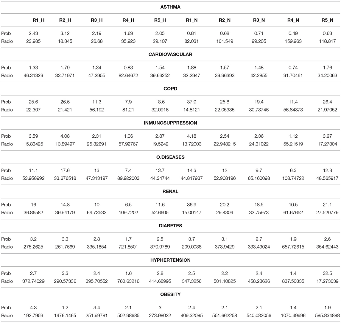
Table 1. Maximum values of probability and radius of the Wigner semicircles, of the 9 comorbidities reported in Mexico.
This study focuses on a particular case in Mexico, but this methodology is indubitably applicable to many countries in the world. One of the approaches proposed in this research is RMT, which originated from John Wishart's analysis of properties in multivariate normal populations [20]. Also in the prediction's in quantum mechanics, the energy levels can be calculated by the eigenvalues together with the RMT elements [21]. In general, the RMTs can work to analyze the multivariate behavior of data as in this study. One of the most important contributions of this document is Wigner and RMT in the comorbidities of patients with COVID-19.
The effect of the COVID-19 pandemic in Mexico has been investigated by some authors, such as Medel-Ramírez et al. [22], which used data mining for data analysis. Parra-Bracamonte et al. [23] analyzed the risk factors for COVID-19 and managed to rank the most determining factors using multivariate logistic regression. In Najera and Ortega-Ávila [24] found a high incidence of comorbidities in deaths that had occurred up to August 2020. In another analysis, Prieto et al. [25] gave predictions on the spread of the pandemic in 2021 using Bayesian inference.
However, as far as we know, there is no study using the methodology presented here that has analyzed the Mexican case. This methodology describes a tool that helps to infer weak convergence: the method of moments in a probability measure. The authors propose applying this method for both deterministic and random probability measures. This article provides an in-depth study of the concepts of weak convergence of probability measures and random probability measures with Wigner's law.
Note that the RMT analysis is in a static setting analysis (refer to Table 1), in the sense, that their entries are not depending on the time. In the interest of studying the evolution of the pandemic over time, which is growing every day in the five regions of Mexico, and the region with the highest risk of contagion in Mexico, this document completes the study with a SuperHeat map resulting from a Machine Learning algorithm which compares by clusters (grouping the lowest scale of infections to the highest density of infections occurred in 176 with the pandemic situation) the risk of the population and their commodities day-by-day who tested positive to COVID-19 in Mexico in the period from 12 April to 5 October 2020 761,665.
The special unitary group of degree n, denoted SU(n), is the Lie group of n x n unitary matrices with determinant 1. The Lie group is used in many applications (for more details refer to Hall [26]). The SU(1) is the simplest case, with only a single element. In this application, we are interested especially in the group SU(2) because it is isomorphic to the group of quaternions of norm 1 and is, thus, diffeomorphic to the 3-sphere, meaning that it can be used to represent rotations in 3-dimensional space, as there is a subjective homomorphism from SU(2) to the rotation group SO(3) with identical symmetry groups [26]. The Lie algebra of SU(2) consists of 2 x 2 skew-Hermitian matrices with trace zero. Mentioned the last properties, note that the Wigner matrices are unit matrices, written in an irreducible unit group (SU), and their rotationally (SO) matrices:
Where Jx, Jy, and Jz are generators of the Lie algebra of the previous groups [27], i.e., there is a non-associative vector of space g, with an alternate bilinear map: g×g→g; (x, y) → [x, y], satisfying the Jacobi identity, which means that the sum of all even permutations is zero. So these three operators are the components of a vector operator, known as angular momentum.
DEFINITION 1 (Hermitian matrix). A square matrix A∈Mn(C) is called a Hermitian matrix if it has the property of A* = A, where A* denotes the conjugate transpose (or Hermitian transpose) of A, i.e., where the subscripts i, j are formally defined by (ai, j) = (āj, i). An important property of these matrices is that each Hermitian matrix is diagonalizable, its eigenvalues are real, and its eigenvectors are 2 x 2 orthogonal.
DEFINITION 2 (Probability Density Function). The probability density function fx(t) of a continuous random variable, is a function whose value at any given sample (or point) in the sample space (the set of possible values taken by the random variable) can be interpreted as providing a relative likelihood that the value of the random variable would equal that sample. A distribution has a density function if and only if its cumulative distribution function FX(x) is continuous. In this case, F is almost everywhere differentiable, and its derivatives can be used as a probability density:
DEFINITION 3 (The empirical measure). Let X1, X2, ... be a sequence of identically distributed independent random variables with values in ℝ. Where P is denoting their probability distribution. The empirical measure Pn is a measurable subset of A⊂ℝ. The empirical distribution function is an estimate of the cumulative distribution function that generated the points in the sample. It converges with probability 1 to that underlying distribution, according to the Glivenko Cantelli theorem. Several results exist to quantify the rate of convergence of the empirical distribution function to the underlying cumulative distribution function:
Where 1A is the indicator function. Note that if it chooses A = [−∞, x], ∀x∈ℝ, then Pn(A) is the distribution of the empirical function.
DEFINITION 4 (Wigner matrix). A Wigner matrix Wn∈Mn(ℂ) is a Hermitian matrix where (Xi, j) with subscripts i<j such that Xi, j are independent and identically randomly distributed variables and are of the complex type with i<j [11] as follows:
• The Xi, j are independent and identically distributed real random variables
• E[Xi, j] = 0, ∀i, j
• if i≠j
•
REMARK 1 (Ensembles of RMT). The main ensembles of RMT, which are called the Gaussian Unitary Ensemble GUE(n) and Gaussian Orthogonal Ensemble GOE(n) and which ensembles are the most classical and most widely studied random matrix ensembles in the literature. The main statistical properties of the eigenvalues of the GOE/GUE random matrices were reviewed, and the random matrices in the Gaussian Unitary Ensembles were found to be invariant under the conjugation of unitary matrices. The entries are independent (up to symmetry) complex centered Gaussian random variables, and the diagonal entries are real centered Gaussian variables with variance 1/N, whereas the diagonal entries can be written as N(0, 1/2)+iN(0, 1/2).
The GUE consider a complex Wigner matrix where Xi, j is the standard complex Gaussian (i.e. Xi, j∽N(0, 1/2)+iN(0, 1/2) and Xi, i∽N(0, 1) (real)), which are defined as follows (for more details refer to Arous and Guionnet [6]):
Let C∈ℂn×n be unitary, so CC* = I and C*WnC have the same distribution as Wn, i.e., (GOE) is invariant under unit conjugation. GOE is a real Wigner matrix where Xi, j∽N(0, 1) and [28].
Where C∈ℝn×n are orthogonal, CCT = I and have the same distribution as Wn, that is, GOE(n) is an invariant function under orthogonal conjugation. Now, the focus is on Gaussian Wigner matrices, whose inputs are Gaussian random variables with zero mean and variance s2 if i≠j and 2s2 if i = j, but this theory only applies to general distributions.
DEFINITION 5 (The Operator Norm for Band Random Matrices). The semicircle law for Wigner band ensembles suggests that in the case of centered entries, the operator norm should asymptotically be of the order of the square root of the bandwidth. It was already observed in Disertori et al. [29] and Valente-Acosta et al. [40] that this cannot hold if the bandwidths do not grow at least at some logarithmic rate with the matrix size.
In the first subsection, Definitions ([Hermitian matrix]-[Wigner matrix]) and the remark [Ensembles of RMT] show positive results in this direction that guarantee an almost certain upper bound on the operator norm that grows proportionally and the bandwidth satisfies some growth condition for centered Wigner band ensembles. The second subsection considers the situation of Wigner band ensembles with arbitrary means and de Finetti band ensembles. The method of the moment was used to obtain the almost certain limit of the appropriately rescaled operator norms for centered Wigner ensembles; then, let M∈Matn×n(C) be a matrix.
The matrix operator norm of M is defined as:
with ||x|| ≤ 1. In that case, x∈Cn and ||.|| ≤ is a normalized vector of Cn.
THEOREM 1 (Bai-Yin Law). The limiting spectral distribution for a Wigner matrix Wn is the upper limit of Bai and Yin [30].
As result, the normalized version is defined as
THEOREM 2 (Semicircle for Wigner Distribution). If the Wn(Wn)n≥1 is a sequence of Wigner matrices, let μn be the probability measure [6]:
In this case, the λ1(Xn) ≤... ≤ λn(Xn)∈ℝ are the eigenvalues of Xn. As a consequence, the μn weakly converges to the semicircle distribution:
One of the most iconic and straightforward tests of the Wigner macroscopic random matrix scale is that it uses the method moments. This approach is based on the intuition that the eigenvalues of the Wigner matrices are distributed according to a limiting law, which is the semicircle distribution μsc. The moments of the empirical distribution μn correspond to sampling moments of the limit distribution, where the number of samples is given by the size of the matrix.
To calculate the k-th moment with the μ-law of a random variable of X, which is the expectation of the E(Xk), the eigenvalues of Xn are denoted by λj(Xn) with an order of λ1(Xn) ≤ λ2(Xn) ≤... ≤ λn(Xn). Note that Xn can be diagonalized since it is a Hermitian matrix. In fact, it has where Dn = diag(λ1(Xn) ≤ λ2(Xn) ≤... ≤ λn(Xn)). Therefore, they are obtained for the k-th moment:
This is a very useful method, especially considering that it does not make any assumptions about the target to measure μn. In the literature on random matrices, this condition is often used as the method of moments (refer to Bai and Yin [30]). In summary, this is the theorem used when applying the method of moments to random matrix theory [31].
The empirical spectral distributions of random matrices, which are K-valued in their entries, have absolute moments of all orders. Then if (mk)k is a sequence of real numbers that satisfy the Carleman condition, then (σn)n converges in expectation to a probability measure μ on (R,B) with moments (mk)k. The k-th random moment is given by a real-valued random variable whose expectation is finite.
The Catalan numbers uniquely determine Wigner's semicircle distribution via its moments, given by:
Cn is the n-th Catalan number, which is given directly by the binomial coefficients:
The Catalan numbers are elements of the sequence of natural numbers. As a result of the semicircle law, it is the unique distribution where the k-th moments are given by the Catalan numbers:
Note that semicircle distribution is uniquely determined by its moments, in other words, the moments of the semicircle are the Catalan number sequence interjected with zeros: 0, 1, 0, 0, 2, 0, 5, 0, 14. Thus, the limit of the k-th moment is measured with the probability distribution with n → ∞ (refer to more details in Random Matrix Theory: A combinatorial Proof of Wigner's Semicircle Law [32]):
However, the Catalan numbers are not only the (even) moments of the semicircle distribution; they also appear as the solution to various combinatorial problems (refer to Achim [33] or Charalambides [34] for examples).
The method of moments for random probability works as follows: If one wants to show weak convergence of random probability measures in expectation, in the probability or almost certainly, it will suffice to show that the random moments converge in expectation, in the probability, or almost certainly.
This section presents a COVID-19 risk analysis for the regions of Mexico. For the record, the database is from the official government web page created by the Secretary of Health in Mexico, available at: https://www.gob.mx/cms/uploads/attachment/file/604001/Datos_abiertos_hist_ricos_2020.pdf.
The Mexico COVID-19 database has the following hierarchical variables (refer to Figure 1): 1) positive patients and negative patients, 2) symptomatic patients, and 3) hospitalized and non-hospitalized patients.
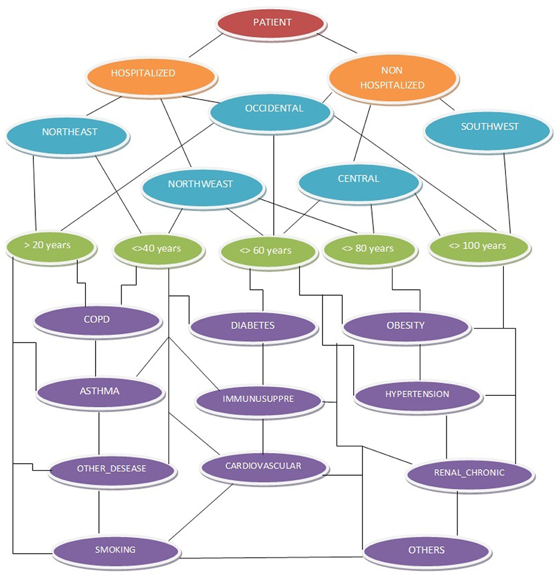
Figure 1. A network database was constructed with hierarchical variables, with the hierarchy level identified by 5 different colors: maroon, orange, blue, green, and purple.
The geographical information of patients infected by the virus in Mexico is divided into 5 regions (refer to shown in blue in Figure 1). Remember that Mexico has 32 federal states, each with a particular political, economic, population, and social situation. The federal states are grouped by regions: Northwest Region (R1), Northeast Region (R2), West Region (R3), Central Region (R4), and Southeast Region (R5). R1 has the following states: Baja California, Baja California Sur, Chihuahua, Sinaloa, and Sonora. In R2 are Coahuila, Durango, Nuevo León, San Luis Potosí, and Tamaulipas. R3 contains Mexico City, the State of Mexico, Guerrero, Hidalgo, Morelos, Puebla, and Tlaxcala. R4 has Aguascalientes, Colima, Guanajuato, Jalisco, Michoacán, Nayarit, Querétaro, and Zacatecas. Finally, R5 covers the states of Campeche, Chiapas, Oaxaca, Quintana Roo, Tabasco, Veracruz, and Yucatán. Symptomatic patients were characterized by presenting the major COVID-19 symptoms, such as cough, sore throat, fever, or shortness of breath. Once the viral detection test was applied, if the patients tested positive, they were classified as positive patients and assumed to have the virus; otherwise, they were considered negative patients. Figure 1 was extracted from the corresponding author's previous study; for more details visit the file repository dataset inputs and their analyses3.
In the first position on the hierarchical variables are positive patients (shown in maroon in Figure 1) these cases have the following subsections: symptom onset date, clinic admission date, and clinic discharge date. In second place are symptomatic patients, who are subsections as hospitalized patients and non-hospitalized patients (shown in orange in Figure 1). For symptomatic patients with severe to critical diseases or those who are severely immunocompromised, health experts admitted them to the clinic immediately and classified them as hospitalized patients in the database. For symptomatic patients with mild to moderate disease who are not severely immunocompromised, the health experts recommended that they must keep a strict quarantine at home and were classified as non-hospitalized patients in the database.
The case study report is based on a comparison of hospitalized and non-hospitalized patients with the patients' comorbidities and their risk of exposure to the virus in different regions of Mexico [35]. These statistical analyses, detail the patients' primary comorbidities (shown in purple in Figure 1), such as diabetes (D) [36], COPD (CO), asthma (A), immunosuppression (IM), hypertension (HY) [37], cardiovascular (CA) problems [38], chronic kidney disease (RE) [39], obesity (OB) [40], and others diseases (OD) [41]. People suffering from any comorbidities are at increased risk of severe COVID-19 infection [40]; the aforementioned diseases play an important role in the recovery potential of patients who have acquired the virus [36–41]. Figure 1 describes Mexico's COVID-19 database extraction and its hierarchical variables. Note that the database analysis period corresponds from 12 April to 5 October 2020 761,665, with a total of 176 daily record files.
The authors propose applying random matrix theory to the probability measure that appears as the limit of the empirical spectral distribution by the Wigner semicircle law of the hierarchical network shown in Figure 1 for every region of Mexico by comorbidities for hospitalized (H) patients and Non-hospitalized (N) patients (refer to Figure 2). Figure 2 is a beautiful graphical representation of the Wigner semicircles overlapping as a result of this proposal, which enables the reader to draw conclusions about the comorbidity of the regions of Mexico and their patients with COVID-19.
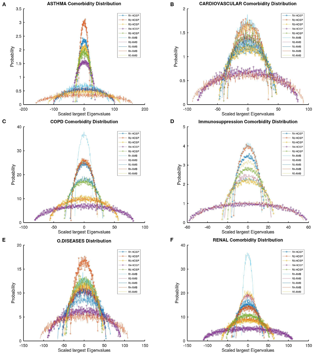
Figure 2. Empirical spectral distribution from the Wigner overlapping semicircular shapes by comorbidities in all regions of Mexico.
In Figure 2A, asthma comorbidity, it can be observed that R2 presents a greater probability of this morbidity in the case of hospitalized patients, while there is a lower probability in non-hospitalized patients. Consequently, the radius of R2 indicates that there are fewer hospitalized than non-hospitalized patients. R1 also has the most cases of hospitalized patients with this comorbidity, R1 has more non-hospitalized patients than R2. The radius in outpatients is more platykurtic than in hospitalized ones since the distribution is more leptokurtic (refer to Table 1).
Table 1 has the local asymptotic values of the local limit from the semicircular Wigner shape distribution, so the reader can compare the analytical values. Note that the x-axis has a scaled largest eigenvalue because it is a semicircle, so it has negative and positive values; the radius indicates the absolute asymptotic value of the eigenvalue distribution.
Figure 2B shows cardiovascular comorbidity; almost all regions and patient types have the same numbers because the radius has similar values, except R4. The radius of R4 indicates that there are more hospitalized and non-hospitalized patients in this region than in other regions but R4 presents a fewer probability of this morbidity than in other regions. Figure 2B shows that R1 presents a greater probability of this morbidity in the case of non-hospitalized patients; Following up to R1 is R2, with the highest probability in hospitalized patients with this comorbidity (refer to Table 1).
Figure 2C shows COPD comorbidity; the probability value in this morbidity is higher than the previous diseases in all cases, and the highest radius is that of R4 in hospitalized patients; as a result, this region of Mexico has the greatest number of patients infected with this morbidity. In Figure 2C, it can be seen that R1 presents the greatest probability of this morbidity in the case of non-hospitalized patients. Next is the R2, with the highest probability in both types of patients (ambulatories and hospitalized); the distribution is leptokurtic for both cases.
In Figure 2D, Immunosuppression comorbidity, it can be observed that R1 presents a greater probability of this morbidity in the case of non-hospitalized patients. Next is R2, which also has the greatest number of cases in hospitalized patients with this comorbidity. The highest radius is that of the R4 in both types of patients. As a result, this region of Mexico has the greatest number of patients infected with this morbidity.
In Figure 2E, for other diseases, it can be observed that R2 presents a greater probability of these comorbidities in the case of non-hospitalized patients. Next is R1, which also has the greatest number of non-hospitalized patients with this comorbidity. The highest radius is that of the R4 in non-hospitalized patients. As a result, this region of Mexico has the greatest number of patients infected with these comorbidities.
In Figure 2F, renal diseases, it can be observed that R1 presents a greater probability of these comorbidities in non-hospitalized patients. Next is R2 with the greatest number of non-hospitalized patients with this comorbidity. The highest radius is that of the R4 in both types of patients. As a result, this region of Mexico has the greatest number of patients infected with this morbidity.
Table 1 is a summary of Mexico's patient regions; with the percentage of patients for each region who have tested positive for COVID-19 but who do not have any type of comorbidity. Of these patients, 61−69% are N patients, while 29−41% were H patients.
This document has a medullary analysis with a SuperHeat map (refer to Figure 3) as a complement to the previous analysis. This SuperHeat map [42] is used as a correlation analysis between the comorbidities of the regions of Mexico and the daily behavior pandemic analysis. Figure 3 is interpreted as follows: it is the dendrogram [42] on its left axis, which indicates in its farthest lines the representation of the highest to the lowest hierarchical correlation, toward the center of the map, the lowest hierarchy appears and its relationship between all elements.
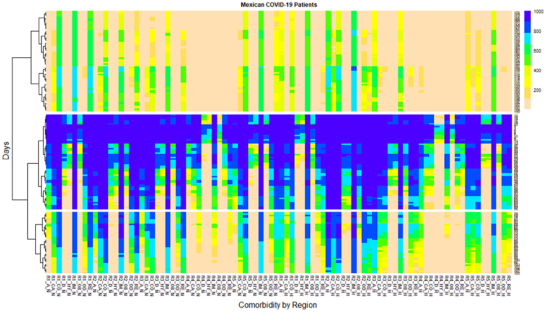
Figure 3. SuperHeat map shows the daily behavior of the pandemic, grouping the lowest scale of infections to the highest density of infections by comorbidities in all regions of Mexico.
Three large groups can be seen on the SuperHeat map, resulting from a Machine Learning algorithm called K-means [43]. This is a type of algorithm clustering characterized by indicating how similar these three groups are, i.e., the similarity coefficient. The similarity coefficient is achieved with a distance called Euclidean Distance [44]. In Figure 3, the right axis indicates the number of days of the pandemic (from 12 April 2019, to 4 October 2020) and the density of infected cases for 176 days. The color scale on the right side of the map indicates the density of infected patients ranging from 1,000 in blue to 200 in pink, corresponding to daily cases.
The SuperHeat has three large groupings or clusterings. The first clustering has the lowest scale of infections approximately 200 days (from day 75 to day 176 during the pandemic). The second clustering has the highest density of infections occurring in the first days of the pandemic, from day 1 to day 50; in this clustering, the N and H patients were infected in practically all regions and all comorbidities, and there were about 1,000 daily cases of contagion (blue) (refer to Figure 3). The third clustering was the result of selecting the days with the highest number of infection transitions, ranging from 1,000 to less than 200 daily infections in all regions and by patient comorbidity type. The third clustering is approximately from day 51 to day 74 of the pandemic in Mexico (refer to Figure 3).
In the first clustering analysis, there are four cases with an average prolongation of the density of N infected patients for a longer period, alternating between 800 and 600 daily infected cases from day 75 to day 176 of the pandemic. As a result, for N patients, R1 patients with COPD, Immunosuppression, and Renal diseases; and N R5 patients with Immunosuppression have an average prolongation of the density of infected patients for the longest time ranging from 800 and 600 daily infected cases of almost 101 days of the pandemic. There are only three cases that are alternating between 800 and 600 daily infected cases, for H patients, R1 patients with Immunosuppression, R2 patients with Asthma, and R2 patients with Immunosuppression. The remaining regions and comorbidities among hospitalized and non-hospitalized patients alternate, with a density of infected patients of approximately 400 and less than 200 daily cases. Note that this clustering has reported the least number of H cases; the majority of infected are N patients, who are recovering at home.
In the second clustering analysis, both N and H patients in all regions have the highest density of infections with around 1,000 daily cases. For N patients, R1 patients with COPD, Immunosuppression, and Renal diseases have an average prolongation of the density for the longest time ranging from 1,000 to 800 infected patients daily for almost 50 days of the pandemic. For H patients, R2 patients with Cardiovascular, COPD, Renal diseases, and Other Diseases; and N patients with Immunosuppression have an average prolongation of the density for a longer time ranging from 1,000 to 800 infected patients daily of almost 50 days of the pandemic. For H patients, R3 patients with Cardiovascular, COPD, Renal diseases, and N with Immunosuppression have an average prolongation of the density for longer periods ranging from 1,000 to 800 patients infected daily for almost 50 days of the pandemic. For H patients, R5 patients with Cardiovascular diseases, COPD, Immunosuppression, and N with Renal diseases have an average prolongation of density for a longer time ranging from 1,000 to 800 infected patients daily for almost 50 days of the pandemic. For H patients, R2 is the only region that has the prolongation of mean density by greater time ranging from 1,000 to 800 infected patients daily for almost 50 days of the pandemic, in comorbidities such as Asthma, Cardiovascular diseases, COPD, and Immunosuppression.
The difficult work in this study is the correct application of all mathematics properties involved in RMTs. This is the main reason for including the two sections in the description of the method (refer to Sections 2.1 and 2.2). The Section 2.3 was written in detail in order that the reader will be able to implement this method. The simulation was programmed in a scripting language in Octave GNU software. A public repository is freely available with the above codes in order to reproduce all the results of this article4.
This article was written in detail so that the reader need not attend the literature review, and includes references for understanding RTMs, Wigner's semicircle law, probability theory, Hermitian random matrices even for the layperson; this is the main reason for including Sections 1.2 and 1.3 in this article.
Note that there are no overlapping semicircle laws from the distribution of randomly oriented graphs in the state of the art, and this is the main contribution of this research. Thus, Figure 2 is a fresh plotting that allows a rapid visual comparison between the local semicircle laws immersed in the plot. Future study will aim to answer the following question: What are the limit dimensions of the matrices where this method can be able to work correctly in large data? Does this method have limits? or even is the technology itself?
This methodology is undoubtedly applicable to many countries in the world, (although this study focuses on a particular case in Mexico). It describes a tool that helps to infer weak convergence using the method of moments in a probability measure. The authors propose applying this method for both deterministic and random probability measures (refer to Table 1).
In Table 1, it can be concluded that COPD comorbidity, renal diseases, and other diseases represent the highest probability in infected hospitalized patients (H). In the case of COPD, renal diseases, and other diseases, Regions 1 and 2 present the highest probability value for hospitalizations. On the other hand, these same comorbidities are also found in non-hospitalized patients, where high levels of probability prevail among those infected.
This research culminates in studying the evolution of the pandemic over time, how it is growing in the five Mexican regions on a day-to-day basis, and the region with the highest risk of contagion in Mexico; this document completes the study with Figure 3 (SuperHeat map), the result of a Machine Learning algorithm which occurring by clusters [grouping the lowest scale of infections to the highest density of infections occurred in the period from 12 April to 5 October 2020 (761,665 Patients)].
From the analysis in Figure 3, it can be concluded that there are four cases with an average prolongation of the density of non-hospitalized infected patients for a longer period, alternating between 800 and 600 new infections daily from day 75 to day 176 of the pandemic are (refer to first clustering): 1) for H patients, R1 patients with COPD, renal disease, 2) for N patients, R1 patients with Immunosuppression, and 3) for N patients, R5 patients with Immunosuppression.
Two cases have the longest time ranging from 800 and 600 new infections daily of almost 101 days: 1) for H patients, R1 patients with Immunosuppression, and 2) for H patients, R2 patients with Asthma and Immunosuppression.
From day 1 to day 50 analysis, it can be concluded that in all regions, both N and H patients, were infected in practically all regions and all comorbidities, and there were about 1,000 daily cases of contagion (refer to second clustering, Figure 3). There are four cases that have the average prolongation of the density of infected patients for the longest time ranging from 1,000 to 800 new infections daily for almost 50 days of a pandemic: 1) for N patients, R1 patients with COPD, Immunosuppression, and Renal diseases, 2) for H patients, R2 patients with Cardiovascular diseases, COPD, Renal diseases, Other Diseases, and for N, R2 patients with Immunosuppression, 3) for H patients, R3 patients with Cardiovascular diseases, COPD, Renal diseases, and for N patients with Immunosuppression, and 4) for H patients, R5 patients with Cardiovascular diseases.
Publicly available datasets were analyzed in this study. This data can be found here: https://www.gob.mx/cms/uploads/attachment/file/604001/Datos_abiertos_hist_ricos_2020.pdf.
ON-J drafted the main manuscript text, prepared all figures, and proposed the comorbidities applications with overlapping Wigner Semicircles. LQ-T, YS-F, and AD-H discussed the review of other studies that use Mexican COVID-19 data. All the authors reviewed and approved the final version of the manuscript.
The authors declare that the research was conducted in the absence of any commercial or financial relationships that could be construed as a potential conflict of interest.
All claims expressed in this article are solely those of the authors and do not necessarily represent those of their affiliated organizations, or those of the publisher, the editors and the reviewers. Any product that may be evaluated in this article, or claim that may be made by its manufacturer, is not guaranteed or endorsed by the publisher.
D, Diabetes; CO, COPD; A, Asthma; IM, Immunosuppression; HY, Hypertension; CA, Cardiovascular; RE, chronic kidney disease; OB, obesity; OD, other diseases; R1, Region 1; R2, Region 2; R3, Region 3; R4, Region 4; R5, Region 5; N, Non-hospitalized patient; H, Hospitalized patient.
1. ^This transmission dynamic modeling is described on: https://www.nature.com/articles/s41598-021-81985-z#Tab1.
2. ^for more details about this research visit our public repository https://github.com/OraliaNJ/RMT_And_Overlapping_Wigner_Semicircles.
3. ^This method describing the Bayesian network and correlation matrices is available on: https://github.com/OraliaNJ/COVID-19_Mex_Analysis.
4. ^Repository available on: https://github.com/OraliaNJ/RMT_And_Overlapping_Wigner_Semicircles.
1. Hui DS, Azhar EI, Madani TA, Ntoumi F, Kock R, Dar O, et al. The continuing 2019-nCoV epidemic threat of novel coronaviruses to global health, The latest 2019 novel coronavirus outbreak in Wuhan, China. Int J Infec Dis. (2020) 91:264–6. doi: 10.1016/j.ijid.2020.01.009
2. Miranda-Novales MG, Vargas-Almanza I, Aragón-Nogales R. COVID-19 por SARS-CoV-2: la nueva emergencia de salud. Revista Mexicana de Pediatr-a. (2020) 86:213–8. doi: 10.35366/91871. Available online at: http://www.scielo.org.mx/pdf/rmp/v86n6/0035-0052-rmp-86-06-213.pdf
3. Perlman S. Another decade, another coronavirus. N Engl J Med. (2020) 382:760–2. doi: 10.1056/NEJMe2001126
4. Capitaine M, Donati-Martin C. Strong asymptotic freeness for Wigner and Wishart matrices. Indiana Univer Math J. (2007). 767–803. doi: 10.48550/arXiv.math/0504414
5. Adamczak R, Chafa D, Wolff P. Circular law for random matrices with exchangeable entries. Random Struct Algor. (2016) 48:454–79. doi: 10.1002/rsa.20599
6. Arous GB, Guionnet A. Wigner matrices. The Oxford Handbook of Random Matrix Theory. (2011). p. 433–51. Available Online at: http://perso.ens-lyon.fr/aguionne/RMTChap21.pdf
7. Dos Santos FC, Federspiel S, Schammo A. Spectral Theory of Random Matrices. University of Luxembourg. Department of Mathematics (2020). Available Online at: https://math.uni.lu/eml/projects/reports/random-matrices.pdf
8. Hirviniemi , Fundamental Properties of Random Hermitian Matrices (2017). Available Online at: https://helda.helsinki.fi/handle/10138/176233
9. O'Rourke S. A note on the Marchenko-Pastur law for a class of random matrices with dependent entries. Electron Commun Prob. (2012) 17:1–13. doi: 10.1214/ECP.v17-2020
10. Valko B,. Lecture 1: Basic random matrix models. University of Wisconsin. Department of Mathematics (2009). Available Online at: http://www.math.wisc.edu/~valko/courses/833/2009f/lec_01.pdf
11. Fleermann M,. Global Local Semicircle Laws for Random Matrices with Correlated Entries (Doctoral Thesis). FernUniversitt in Hagen at the Faculty of Mathematics Computer Science (2019). Available Online at: https://ub-deposit.fernuni-hagen.de/receive/mir_mods_00001524
12. Bouchaud MJP,. Chaos multiplicatif Gaussien, matrices aléatoires et applications (Doctoral Thesis). Dauphine Université Paris at the Faculty of Mathematics (2012). Available Online at: http://www.normalesup.org/~allez/THESE_ARTICLE.pdf
13. Erdõs L, Yau HT. A comment on the Wigner-Dyson-Mehta bulk universality conjecture for Wigner matrices. Electron J Prob. (2012) 17:1–5. doi: 10.48550/arXiv.1201.5619
14. Erdõs L. Universality of Wigner random matrices: a survey of recent results. Russian Math Surveys. (2011). 66:507. doi: 10.48550/arXiv.1004.0861
15. Shang Y. On the skew-spectral distribution of randomly oriented graphs. arXiv preprint. (2017). doi: 10.48550/arXiv.1702.02304
17. Melo M,. Applications of Random Matrices to Image Processing for Image Denoising (2015). Available Online at: http://hdl.handle.net/11141/736.
19. Namaki A Raei R Ardalankia J Hedayatifar L Hosseiny A Haven E and Jafari GR. Analysis of the global banking network by random matrix theory. Front in Phys-Lausanne (2021) 18:608. doi: 10.3389/fphy.2020.586561
20. Masucci AM,. Moments method for random matrices with applications to wireless communication (Doctoral Thesis). CentraleSupélec Université Paris at the Faculty of Physics (2011). Available Online at: https://tel.archives-ouvertes.fr/tel-00805578/
21. Benaych-Georges F, Knowles A. Lectures on the local semicircle law for Wigner matrices. preprint arXiv. (2018). doi: 10.48550/arXiv.1601.04055
22. Medel-Ramírez C, Medel-López H. Data Mining for the Study of the Epidemic (SARS-CoV-2) COVID-19: Algorithm for the Identification of Patients (SARS-CoV-2) COVID 19 in Mexico (June 3, 2020). Available Online at: https://ssrn.com/abstract=3619549
23. Parra-Bracamonte GM, Lopez-Villalobos N, Parra-Bracamonte FE. Clinical characteristics and risk factors for mortality of patients with COVID-19 in a large data set from Mexico. Ann Epidemiol. (2020) 52:93–98. doi: 10.1016/j.annepidem.2020.08.005
24. Najera H, Ortega-Ávila AG. Health and Institutional Risk Factors of COVID-19 Mortality in Mexico, 2020. Am J Prev Med. (2021) 60:471–7. doi: 10.1016/j.amepre.2020.10.015
25. Prieto K, Chavez-Hernandez M, Romero-Leiton JP. On mobility trends analysis of COVID-19 dissemination in Mexico City. medRxiv. (2021). doi: 10.1101/2021.01.24.21250406
26. Hall BC. Lie Groups, Lie Algebras, and Representations: An Elementary Introduction. New York, NY: Springer (2003).
27. Porikli F, Tuzel O, Meer P. Covariance tracking using model update based on lie algebra. IEEE Comput Soc Conf Comput Vis Pattern Recogn. (2006) 1:728–35. doi: 10.1109/CVPR.2006.94
28. Tracy CA, Widom H. The distribution of the largest eigenvalue in the Gaussian ensembles: = 1, 2, 4. In: Calogero Moser Sutherland Models. New York, NY: Springer (2000). p. 461–72.
29. Disertori M, Pinson H, Spencer T. Density of states for random band matrices. Commun Math Phys. (2002) 232:83–124. doi: 10.1007/s00220-002-0733-0
30. Bai ZD, Yin YQ. Necessary and sufficient conditions for almost sure convergence of the largest eigenvalue of a Wigner matrix. Ann Probab. (1988) 16:1729–41.
31. Anderson GW, Guionnet A, Zeitouni O. An introduction to Random Matrices (No. 118). Cambridge: Cambridge University Press (2010).
32. Wolf V, Random Matrix Theory: A Combinatorial Proof of Wigner's Semicircle Law. Scripps Senior Theses. Department of Mathematics of Women's College in Claremont California (2021). Available Online at: https://scholarship.claremont.edu/scripps_theses/1683
33. Achim K. Wahrschein-Lichkeits-Theorie. Springer (2013). Available Online at: https://link.springer.com/book/10.1007%2F978-3-642-36018-3
34. Charalambides CA. Enumerative Combinatorics. New York, NY: CRC Press (2018). doi: 10.1201/9781315273112. Available online at: https://www.taylorfrancis.com/books/mono/10.1201/9781315273112/enumerative-combinatorics-charalambos-charalambides
35. Jordan RE, Adab P, Cheng K. COVID-19: risk factors for severe disease and death. BMJ. (2020) 368:m1198. doi: 10.1136/bmj.m1198
36. Nolasco-Jáuregui O, Quezada-Tállez LA, Rodríguez-Torres EE, Tetrlalmatzi-Montiel M. COVID-19 Patients analysis using superheat map and bayesian network to identify comorbidities correlations under different scenarios. J Infect Dis Ther. (2021) 9:S5. doi: 10.1101/2021.05.11.21257055
37. Fang L, Karakiulakis G, Roth M. Are patients with hypertension and diabetes mellitus at increased risk for COVID-19 infection?. Lancet Respiratory Med. (2020) 8:21. doi: 10.1590/S1806-37132013000400015
38. Phelps M, Christensen DM, Gerds T, Fosbl E, Torp-Pedersen C, Schou M, et al. Cardiovascular comorbidities as predictors for severe COVID-19 infection or death. Eur Heart J Quality Care Clin Outcomes. (2021) 7:172–80. doi: 10.1093/ehjqcco/qcaa081
39. Bansal M. Cardiovascular disease and COVID-19. Diabet Metab Syndrome. (2020) 14:247–50. doi: 10.1016/j.dsx.2020.03.013
40. Valente-Acosta B, Hoyo-Ulloa I, Espinosa-Aguilar L, Mendoza-Aguilar R, Garcia-Guerrero J, Ontanon-Zurita D, et al. COVID-19 severe pneumonia in Mexico City-First experience in a Mexican hospital. medRxiv. (2020). doi: 10.1101/2020.04.26.20080796
41. Kassir R. Risk of COVID-19 for patients with obesity. Obes Rev. (2020) 21:e13034. doi: 10.1111/obr.13034
42. Barter RL, Yu B. Superheat: an R package for creating beautiful and extendable heatmaps for visualizing complex data. J Comp Grap Stat. (2018) 27:910–22. doi: 10.1080/10618600.2018.1473780
43. Wu L, Peng Y, Fan J, Wang Y, Huang G. A novel kernel extreme learning machine model coupled with K-means clustering and firefly algorithm for estimating monthly reference evapotranspiration in parallel computation. Agr Water Manag. (2021) 245:106624. doi: 10.1016/j.agwat.2020.106624
44. Lange M, Zühlke D, Holz O, Villmann T, Mittweida SG. April. Applications of lp-Norms and their smooth approximations for gradient based learning vector quantization. In: European Symposium on Artificial Neural Networks, Computational Intelligence and Machine Learning. Bruges (2014). p. 271–6. Available Online at: http://citeseerx.ist.psu.edu/viewdoc/download?doi=10.1.1.642.3159&rep=rep1&type=pdf
Keywords: random matrix theory, COVID-19, Wigner's law, multivariate distribution, SuperHeat map, eigenvalue distribution
Citation: Nolasco-Jáuregui O, Quezada-Téllez LA, Salazar-Flores Y and Díaz-Hernández A (2022) Application of Random Matrix Theory With Maximum Local Overlapping Semicircles for Comorbidity Analysis. Front. Appl. Math. Stat. 8:848898. doi: 10.3389/fams.2022.848898
Received: 05 January 2022; Accepted: 06 April 2022;
Published: 02 June 2022.
Edited by:
Li Xing, University of Saskatchewan, CanadaReviewed by:
Yilun Shang, Northumbria University, United KingdomCopyright © 2022 Nolasco-Jáuregui, Quezada-Téllez, Salazar-Flores and Díaz-Hernández. This is an open-access article distributed under the terms of the Creative Commons Attribution License (CC BY). The use, distribution or reproduction in other forums is permitted, provided the original author(s) and the copyright owner(s) are credited and that the original publication in this journal is cited, in accordance with accepted academic practice. No use, distribution or reproduction is permitted which does not comply with these terms.
*Correspondence: Oralia Nolasco-Jáuregui, b3JhbGlhbm9sYXNjby5qYXVyZWd1aUBnbWFpbC5jb20=
Disclaimer: All claims expressed in this article are solely those of the authors and do not necessarily represent those of their affiliated organizations, or those of the publisher, the editors and the reviewers. Any product that may be evaluated in this article or claim that may be made by its manufacturer is not guaranteed or endorsed by the publisher.
Research integrity at Frontiers
Learn more about the work of our research integrity team to safeguard the quality of each article we publish.