 Mohamed R. Abonazel
 Issam Dawoud
 Fuad A. Awwad
 Adewale F. Lukman
95% of researchers rate our articles as excellent or good
Learn more about the work of our research integrity team to safeguard the quality of each article we publish.
Find out more
ORIGINAL RESEARCH article
Front. Appl. Math. Stat. , 22 February 2022
Sec. Optimization
Volume 8 - 2022 | https://doi.org/10.3389/fams.2022.775068
This article is part of the Research Topic 2022 Applied Mathematics and Statistics – Editor’s Pick View all 15 articles
The linear regression model becomes unsuitable when the response variable is expressed as percentages, proportions, and rates. The beta regression (BR) model is more appropriate for the variable of this form. The BR model uses the conventional maximum likelihood estimator (BML), and this estimator may not be efficient when the regressors are linearly dependent. The beta ridge estimator was suggested as an alternative to BML in the literature. In this study, we developed the Dawoud–Kibria estimator to handle multicollinearity in the BR model. The properties of the new estimator are derived. We compared the performance of the estimator with the existing estimators theoretically using the mean squared error criterion. A Monte Carlo simulation and a real-life application were carried out to show the benefits of the proposed estimator. The theoretical comparison, simulation, and real-life application results revealed the superiority of the proposed estimator.
The linear regression (LR)model is used if the dependent variable follows a normal distribution. The assumption of the normality of the dependent variable may be violated and then it will fit some of the exponential family distributions as a negative binomial, Poisson, gamma, inverse Gaussian, and beta, so in this case, we use the generalized linear (GL) model instead of the LR model. The beta regression (BR) model is applied in many different fields such as engineering, medical sciences, physical sciences, social sciences, environment, and business if the dependent variable observations are between (0, 1). To estimate the BR model parameters, we use the maximum likelihood (ML) estimator which is more convenient than the ordinary least squares (OLS) estimator for describing and investigating different phenomena.
In the LR model, the explanatory variables may be correlated and this causes a problem called multicollinearity in which this problem may arise in the BR model. The ML estimator is the most popular used method for estimating the unknown regression parameters in the BR model. But also, in the existence of multicollinearity problems, the regression parameters' variances and standard errors are very large. To reduce the multicollinearity effect, different biased estimation methods are proposed and the most popular method is the ordinary ridge regression (ORR) estimation method which was proposed by Hoerl and Kennard [1, 2]. Another recent one parameter estimator proposed by Kibria and Lukman [3] to solve the multicollinearity is the Kibria and Lukman estimator. Also, in the case of an estimator with two parameters, Özkale and Kaçiranlar [4] proposed a two-parameter estimator. Very recently, Dawoud and Kibria [5] proposed a new kind of two-parameter estimator called the Dawoud–Kibria (DK) estimator. There are other recent studies regarding the one parameter and two-parameter estimators in LR and GL models, such as Roozbeh et al. [6], Lukman et al. [7], Arashi et al. [8], Farghali et al. [9], Lukman et al. [10, 11], Algamal and Abonazel [12], Akram et al. [13], and Abonazel et al. [14]. In this article, we drive the Dawoud–Kibria estimator for the BR model in the presence of the multicollinearity problem. Then, the properties of the Dawoud–Kibria estimator for the BR model are investigated.
This article is organized as follows. The methodology and the proposed estimator are given in section methodology. In section the superiority of the proposed estimator, the theoretical comparisons among the estimators are conducted. Section selection of biasing parameters k and d gives the proposed biasing parameters for the estimators. In sections Monte Carlo simulation study and real data application, the Monte Carlo simulation and the real-life dataset results are presented. Finally, in section conclusion, some conclusions of this article are given.
In this section, we discuss the BR model. Then, the ridge, Kibria–Lukman, and Özkale–Kaçiranlar estimators are stated to the BR model. After that, we introduce the Dawoud–Kibria estimator for the BR model. Finally, the biasing parameters of the Dawoud–Kibria estimator for the BR model are proposed.
The BR model is popularly used in many different fields such as economics and medical studies. The BR model is used to show the effect of explanatory variables on a non-normal response variable as any generalized LR model. However, the response variable for the BR model is restricted to the interval (0, 1) as rates, proportions, and fractions. The BR model was given firstly by the authors Ferrari and Cribari-Neto [15] with relating the response variable mean function to linear predictors set through a link function. The BR model has a precision parameter where its reciprocal is determined as a dispersion measure [16, 17].
Let y be a continuous random variable having a beta distribution, then the probability density function of y is given as:
where Γ(·) is called as the gamma function and ϕ is called as the precision parameter. The beta probability distribution mean and variance are as follows:
Let y1, …, yn be independent random variables, where each yi; i = 1, …, n follows the density in Equation (1) with mean μi and unknown precision ϕ. The model is obtained by assuming that the mean of yi can be written as:
where g(·) is the used link function, is an (p × 1) unknown parameters vector, is the vector of p regressors, and ηi is the linear predictor.
The BR parameters estimation is done using the beta maximum likelihood (BML) method [18]. The BR log-likelihood function is given as:
Differentiating the log-likelihood given in Equation (3) with respect to the parameter β provides us the score function of the parameter β that is given as:
where ; with g′(·) is the first derivative of g(·); with , and ; with , such that ψ(·) denoting the digamma function. The iterative reweighted least-squares (IRLS) algorithm or the Fisher scoring algorithm are used for estimating the parameter β [19, 20]. This algorithm form is given as:
where is called the score function, and is called the information matrix for β, for more details, see Espinheira et al. [20]. With the use of the IRLS algorithm with initial values of β and ϕ as in Ferrari and Cribari-Neto [15] and Espinheira et al. [20], the BML estimator of the parameter β is provided as:
where X is an (n × p) design matrix, , and Ŵ = diag(ŵ1, …, ŵn); with
Here, and are the estimates of W, T, μi, and μ*, respectively, evaluated at the ML estimator of β and ϕ [15].
Now, let , and where γ1 ≥ … ≥ γp ≥ 0 and Q is the matrix whose columns are the eigenvectors of the (X′ŴX) matrix. Then, the mean squared error matrix (MSEM) and the mean squared error (MSE) of an estimator are defined as follows:
Then the MSEM and MSE of are.
To reduce the effects of multicollinearity in the BR model, Abonazel and Taha [21] and Qasim et al. [22] introduced the BRR estimator as an alternative to the BML estimator and is given as:
The MSEM and MSE of are
where L = (Γ + k Ip) and Lj = (γj + k).
The BKL estimator is defined as follows:
The MSEM and MSE of are
where N = (Γ − k Ip) and Nj = (γj − k).
Recently, Abonazel et al. [14] proposed the BOK estimator as an extension of the Özkale and Kaçiranlar [4] estimator in the BR model and is defined as follows:
The MSEM and MSE of are
where G = (Γ + kd Ip) and Gj = (γj + kd).
Extensions of the two-parameter estimators to the area of GLMs have been recently developed; such as Qasim et al. [22], Farghali et al. [9], Lukman et al. [23], Algamal and Abonazel [12], and Abonazel et al. [14]. Following the previous works, we introduced the beta version of the two-parameter estimator of Dawoud and Kibria [5] (BDK) as follows:
We give the MSEM of the proposed as follows:
where M = (Γ + k(1 + d)Ip), R = (Γ − k(1 + d)Ip), Mj = (γj + k(1 + d)) and Rj = (γj − k(1 + d)).
Theorem 1: If , then .
Proof: The MSE difference between the BML and the BDK estimators is written as
In the case of in the equation (23), it implies that , then . That means the BDK estimator is better than the BML estimator if .
Theorem 2: If ,
then
Proof: The MSE difference between the BRR and the BDK estimators is written as
In the case of in the Equation (24), it implies that , then . That means the BDK estimator is better than the BRR estimator if .
Theorem 3: If .
then
Proof: The MSE difference between the BKL and the BDK estimators is written as
In the case of in the Equation (25), it implies that , then . That means the BDK estimator is better than the BKL estimator
if .
Theorem 4: If ,
then
Proof: The MSE difference between the BOK and the BDK estimators is written as
In the case of in the Equation (26), it implies that , then . That means the BDK estimator is better than the BOK estimator if .
We will suggest the following biasing parameters' estimators for the mentioned estimators.
Following Hoerl et al. [24] and Qasim et al. [22], of the BRR estimator is written as
where is the jth element of vector and is the ML estimate of ϕ [15].
- Following Lukman et al. [25], of the BKL estimator is written as
- Following Özkale and Kaçiranlar [4] and Abonazel et al. [14], and of the BOK estimator are written as
- Following Dawoud and Kibria [5], we suggest two different of the proposed BDK estimator as follows:
In this section, a Monte Carlo simulation study has been conducted to compare the performances of BML, BRR, BKL, and BOK with the suggested estimator (BDK). The program of the simulation study is written in R programming language based on the betareg package.
We simulated the datasets with the following settings:
1) The response variable yi is generated from the beta distribution as Beta (μi, ϕ), where ; i = 1, …, n, and xi is the ith row of X. The precision parameter ϕ chosen in the simulation is ϕ = 2 and 6.
2) Sample size: n = 50, 75, 100, 150, and 200.
3) Explanatory variables are generated with a degree of multicollinearity as in Kibria [26]: where uij are the independent standard uniform pseudorandom numbers, and ρ is defined as the correlation between the explanatory variables, ρ = 0.80, 0.85, 0.90, 0.95, and 0.99.
4) The number of explanatory variables is p = 2, 4, and 6; with β′ β = 1 and β1 = … = βp, as per Kaçiranlar and Dawoud [27], Rady et al. [28], Abonazel and Farghali [29], Farghali et al. [9], Dawoud and Abonazel [30], and Awwad et al. [31].
5) We used the simulated MSE (SMSE) criterion for verification, which are computed as
where is the estimated value vector at the lth experiment of the simulation, β is the true parameter vector. The number of replications is 5,000.
We have the following comments according to the simulation results in Tables 1–6: Obviously, from Tables 1–6, the proposed estimator possesses a smaller SMSE than the BML estimator and other estimators understudy for all sample sizes. For instance, from Table 3, when ρ = 0.9, n = 50, the SMSE of BML is 16.331 while the SMSE for other estimators is as follows: 13.295 (BRR), 13.254 (BKL), 10.640 (BOK), 4.493 (BDK(1)), and 4.428 (BDK(2)), respectively. Similarly, when the values of ϕ increase the SMSE also increases: from Table 1, when ϕ = 2, n = 100 and ρ = 0.99, and Table 2, when ϕ = 6, n = 100 and ρ = 0.99, the SMSE of BRR rises from 102.758 to 252.353. Also, it is evident that the SMSE values of all the estimators increased as the number of explanatory p increased. For the one-parameter shrinkage estimator, the BKL estimator consistently dominates the BRR estimator. For two-parameter shrinkage estimators, the BDK estimator dominates the BOK estimator. Overall, the BDK dominates both the one-parameter and the two-parameter estimators. However, the performance of each estimator is a function of the employed shrinkage parameter.
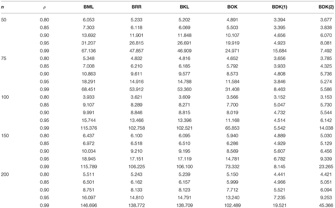
Table 1. Simulated mean square error (SMSE) values of different estimators when p = 2 and ϕ = 2.
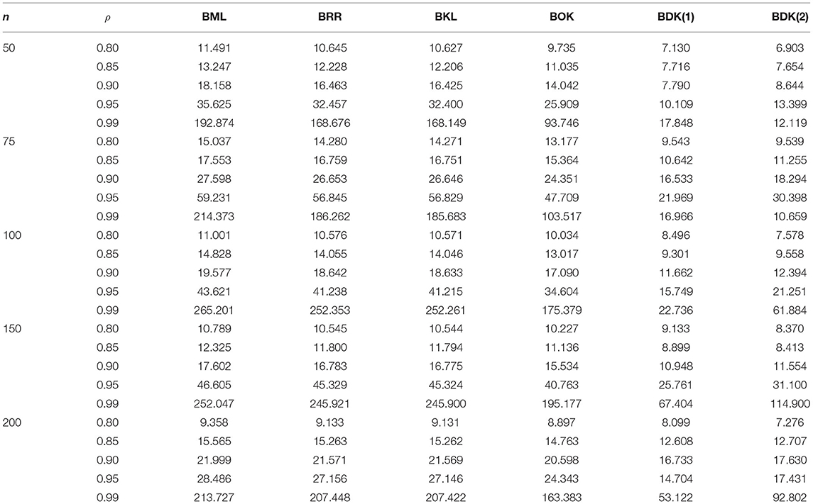
Table 2. SMSE values of different estimators when p = 2 and ϕ = 6.
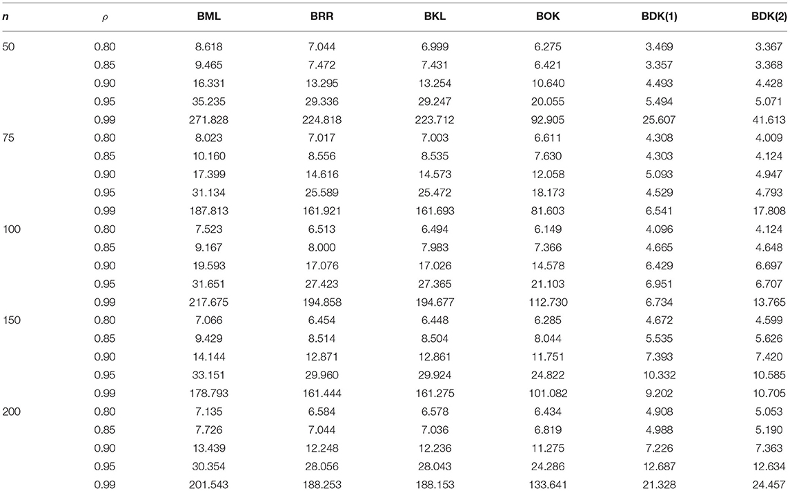
Table 3. SMSE values of different estimators when p = 4 and ϕ = 2.
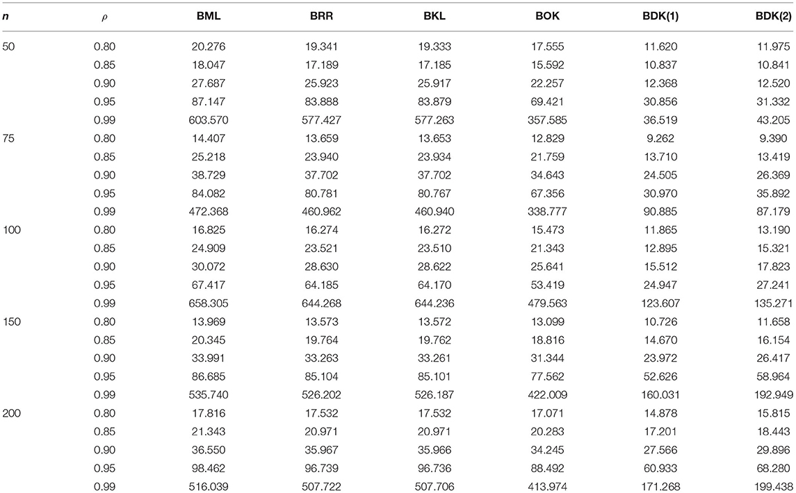
Table 4. SMSE values of different estimators when p = 4 and ϕ = 6.

Table 5. SMSE values of different estimators when p = 6 and ϕ = 2.
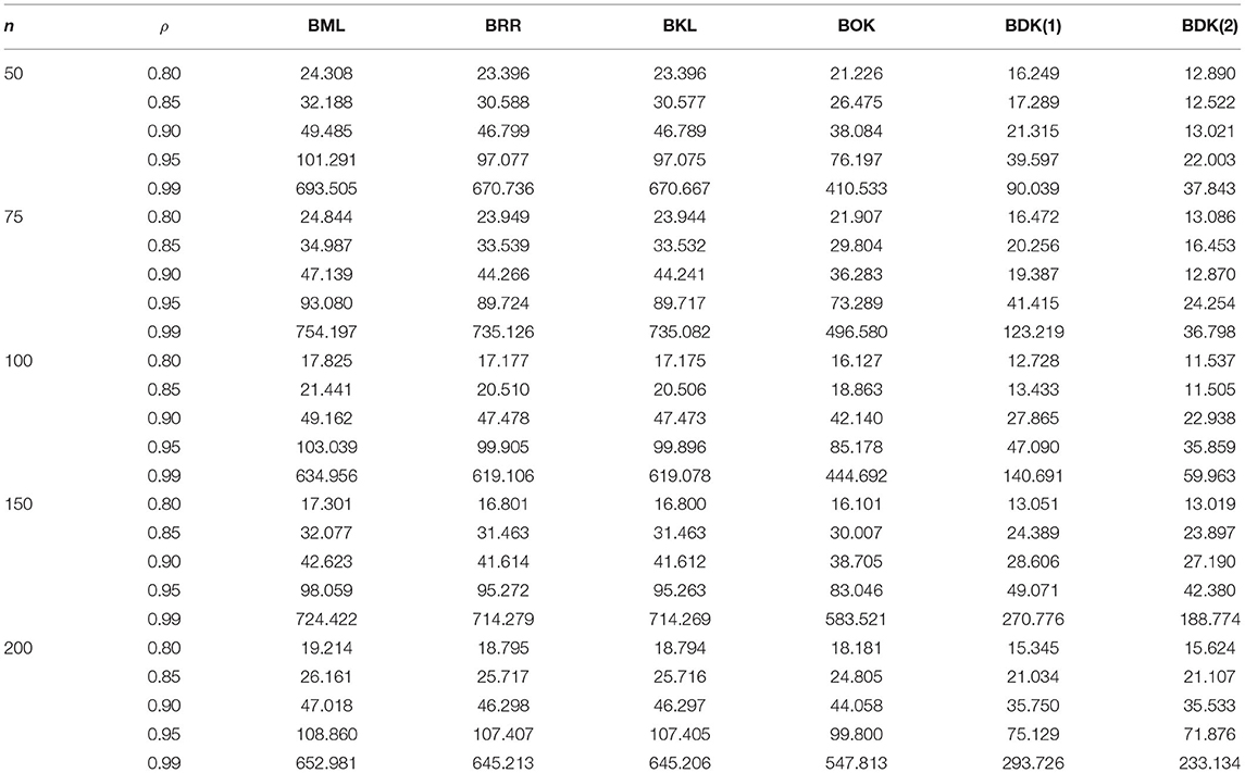
Table 6. SMSE values of different estimators when p = 6 and ϕ = 6.
The implementation of the proposed estimator is illustrated by a study applied to the well-being index of Turkey in 2015 [32]. The index involves the aspects of accommodation, jobs, income and wealth, health, education, climate, protection, public engagement and access to community resources and social life. As the life satisfaction index is between 0 and 1. The values close to 1 refer to a better standard of living. The data are obtained from the Turkish Statistics Association. The original dataset consists of some dimensions that are represented by 41 indicators. Here, we are interested in only nine indicators used by Abonazel and Taha [21] and the number of observations is 50. The response variable is the level of happiness and eight explanatory variables are x1: Number of rooms per person, x2: Average point of necessary placement scores of the system for transition to secondary education from basic education, x3: Satisfaction rate with public education services, x4: Percentage of the population receiving waste services, x5: Satisfaction rate with public safety services, x6: The access rate of the population to sewerage and pipe system, x7: Satisfaction rate with public health services, and x8: Percentage of households declaring to fail on meeting basic needs.
To investigate the multicollinearity through correlation coefficients between the explanatory variables, a visualization of the correlation matrix of the variables is constructed with the corresponding coefficients reported in Figure 1. The correlation coefficients indicate that there are strong relationships (more than 0.8) between some explanatory variables. This denotes the severe multicollinearity presence. Moreover, this conclusion is confirmed by the variance inflation factor (VIF) and the condition number [33]; where the VIFs of the eight explanatory variables are 7.5, 6.1, 10.8, 10.1, 9.1, 9.8, 9.7, and 4.3, respectively, and the CN is 3,936.055.
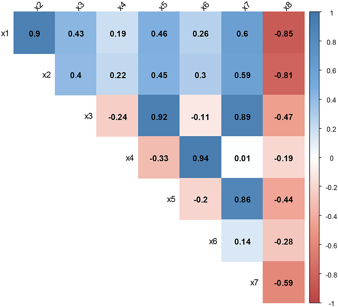
Figure 1. Visualization of the correlation matrix.
Table 7 provides the regression parameter estimates for the BR model using BML, BRR, BKL, BOK, and BDK. From Table 7, it can note that the estimated regression parameters of all estimators have the same signs (except x1 and x2 in BDK(2) only); this means that the type of relationship between each explanatory variable and the response variable is not changed from what it was in the BML. The estimated MSE of the five estimators were obtained by Equations (10), (13), (16), (19), and (22), respectively. The results of Table 7 indicate that the estimated MSE value of BML is greater than the estimated MSE values of BRR, BKL, BOK, and BDK estimators. Moreover, the MSE values of BDK(1) and BDK(2) estimators are lower than other estimators, which means that the BDK estimator achieves the best performance. Furthermore, in terms of the prediction, the R2 value of the proposed estimator (BDK) is the greatest among all the used estimators. To further highlight the performance of the BDK estimator, generalized cross-validation (GCV) criterion is used in comparison [8, 34, 35]. Regarding GCV values, it can note that the BDK yielded the least value compared with other estimators.
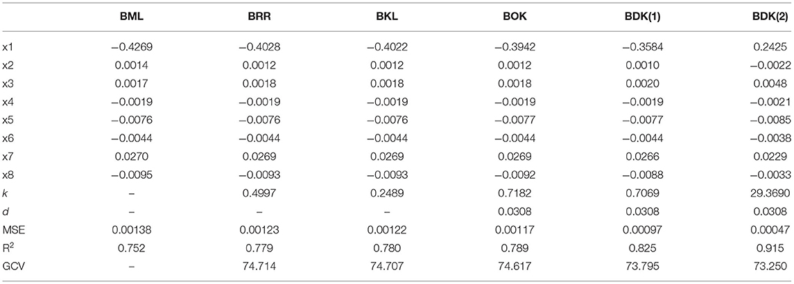
Table 7. Estimation results for the used estimators.
Through this application, we verify the theoretical results as follows:
1. Since the condition is satisfied, then the BDK estimator is better than the BML estimator.
2. Since the condition is satisfied, then the BDK estimator is better than the BRR estimator.
3. Since the condition is satisfied, then the BDK estimator is better than the BKL estimator.
4. Since the condition is satisfied, then the BDK estimator is better than the BOK estimator.
Regression modeling describes the relationship that exists between a dependent variable and one or more explanatory variables. Linear dependency, a situation called multicollinearity, is a common problem with two or more explanatory variables. Multicollinearity is a threat to the efficiency of the maximum likelihood estimator in both the linear and generalized linear models, such as the BR model. The ridge regression estimator serves as an alternative to the maximum likelihood estimator for parameter estimation in the beta regression model. In this article, we developed the BDK estimator and compared its performance theoretically with some other estimators. A simulation study has been conducted to compare the performance of the estimators. Real-life data have been analyzed to illustrate the findings of the article. We concluded that the BDK estimator proposed in this articles generally preferred when there is multicollinearity in the beta regression model. For future work, for example, one can use new methods to select the shrinkage parameters as an extension to Uslu et al. [36] and Inan et al. [37] in the BR model, or provide robust biased estimators for handling multicollinearity and outliers together in the beta regression model as an extension to Awwad et al. [31] and Dawoud and Abonazel [30].
The raw data supporting the conclusions of this article will be made available by the authors, without undue reservation.
MA, ID, and FA contributed to conception and structural design of the manuscript. MA performed the simulation and application sections. AL wrote the abstract and conclusion sections of the manuscript. All authors contributed to manuscript revision, read, and approved the submitted version.
The authors declare that the research was conducted in the absence of any commercial or financial relationships that could be construed as a potential conflict of interest.
All claims expressed in this article are solely those of the authors and do not necessarily represent those of their affiliated organizations, or those of the publisher, the editors and the reviewers. Any product that may be evaluated in this article, or claim that may be made by its manufacturer, is not guaranteed or endorsed by the publisher.
The authors would like to thank the Deanship of Scientific Research at King Saud University represented by the Research Center at CBA for supporting this research financially.
1. Hoerl AE, Kennard RW. Ridge regression: biased estimation for non-orthogonal problems. Technometrics. (1970) 12:55–67. doi: 10.1080/00401706.1970.10488634
2. Hoerl AE, Kennard RW. Ridge regression: applications to non-orthogonal problems. Technometrics. (1970) 12:69–82. doi: 10.1080/00401706.1970.10488635
3. Kibria BMG, Lukman AFA. New ridge-type estimator for the linear regression model: simulations and applications. Scientifica. (2020) 2020:9758378. doi: 10.1155/2020/9758378
4. Özkale MR, Kaçiranlar S. The restricted, and unrestricted two-parameter estimators. Commun Stat Theory Methods. (2007) 36:2707–25. doi: 10.1080/03610920701386877
5. Dawoud I, Kibria BMG. A new biased estimator to combat the multicollinearity of the gaussian linear regression model. Stat J. (2020) 3:526–41. doi: 10.3390/stats3040033
6. Roozbeh M, Arashi M, Hamzah NA. Generalized cross-validation for simultaneous optimization of tuning parameters in ridge regression. Iran J Sci Technol Trans A Sci. (2020) 44:473–85. doi: 10.1007/s40995-020-00851-1
7. Lukman AF, Ayinde K, Kibria GBM, Adewuyi E. Modified ridge-type estimator for the gamma regression model. Commun Stat Simul Comput. (2020). doi: 10.1080/03610918.2020.1752720
8. Arashi M, Roozbeh M, Hamzah NA, Gasparini M. Ridge regression and its applications in genetic studies. PloS One. (2021) 16:e0245376. doi: 10.1371/journal.pone.0245376
9. Farghali RA, Qasim M, Kibria BG, Abonazel MR. Generalized two-parameter estimators in the multinomial logit regression model: methods, simulation and application. Commun Stat Simul Comput. (2021) 1−16. doi: 10.1080/03610918.2021.1934023
10. Lukman AF, Aladeitan B, Ayinde K, Abonazel MR. Modified ridge-type for the Poisson regression model: simulation and application. J Appl Stat. (2021). 1−13. doi: 10.1080/02664763.2021.1889998
11. Lukman AF, Issam D, Kibria GBM, Zakariya A, Aladeitan B. A new ridge-type estimator for the gamma regression model. Scientifica. (2021) 2021:1–8. doi: 10.1155/2021/5545356
12. Algamal ZY, Abonazel MR. Developing a Liu-type estimator in beta regression model. Concurrency Comput Pract Exp. (2021) 34:e6685. doi: 10.1002/cpe.6685
13. Akram MN, Amin M, Elhassanein A, Ullah MA. A new modified ridge-type estimator for the beta regression model: simulation and application. AIMS Math. (2022) 7:1035–57. doi: 10.3934/math.2022062
14. Abonazel MR, Algamal ZY, Awwad FA, Taha IM. A new two-parameter estimator for beta regression model: method, simulation, and application. Front Appl Math Stat. (2022) 7:780322. doi: 10.3389/fams.2021.780322
15. Ferrari S, Cribari-Neto F. Beta regression for modelling rates and proportions. J Appl Stat. (2004) 31:799–815. doi: 10.1080/0266476042000214501
16. Algamal ZY. A particle swarm optimization method for variable selection in beta regression model. Electron J Appl Stat Anal. (2019) 12:508–19.
17. Mahmood SW, Seyala NN, Algamal ZY. Adjusted R2-type measures for beta regression model. Electron J Appl Stat Anal. (2020) 13:350–7. doi: 10.1285/i20705948v13n2p350
18. Espinheira PL, Ferrari SL, Cribari-Neto F. On beta regression residuals. J Appl Stat. (2008) 35:407–19. doi: 10.1080/02664760701834931
19. Espinheira PL, da Silva LCM, Silva ADO. Prediction Measures in Beta Regression Models. arXiv preprint arXiv:1501.04830 (2015).
20. Espinheira PL, da Silva LCM, Silva ADO, Ospina R. Model selection criteria on beta regression for machine learning. Mach Learn Knowl Extraction. (2019) 1:427–49. doi: 10.3390/make1010026
21. Abonazel MR, Taha IM. Beta ridge regression estimators: simulation and application. Commun Stat Simul Comput. (2021) 1−13. doi: 10.1080/03610918.2021.1960373
22. Qasim M, Månsson K, Golam Kibria BM. On some beta ridge regression estimators: method, simulation and application. J Stat Comput Simul. (2021) 91:1699–712. doi: 10.1080/00949655.2020.1867549
23. Lukman AF, Adewuyi E, Månsson K, Kibria GBM. A new estimator for the multicollinear Poisson regression model: simulation and application. Sci Rep. (2021) 11:3732. doi: 10.1038/s41598-021-82582-w
24. Hoerl AE, Kennard RW, Baldwin KF. Ridge regression: some simulations. Commun Stat Theory Methods. (1975) 4:105–23. doi: 10.1080/03610917508548342
25. Lukman AF, Ayinde K, Binuomote S, Onate AC. Modified ridge-type estimator to combat multicollinearity: application to chemical data. J Chemometr. (2019) 33:e3125. doi: 10.1002/cem.3125
26. Kibria BG. Performance of some new ridge regression estimators. Commun Stat Simul Comput. (2003) 32:419–35. doi: 10.1081/SAC-120017499
27. Kaçiranlar S, Dawoud I. On the performance of the Poisson and the negative binomial ridge predictors. Commun Stat Simul Comput. (2018) 47:1751–70. doi: 10.1080/03610918.2017.1324978
28. Rady EA, Abonazel MR, Taha IM. A new biased estimator for zero-inflated count regression models. J Mod Appl Stat Methods. (2019). Available online at: https://www.researchgate.net/publication/337155202_A_New_Biased_Estimator_for_Zero-Inflated_Count_Regression_Models
29. Abonazel MR, Farghali RA. Liu-Type multinomial logistic estimator. Sankhya B. (2019) 81:203–25. doi: 10.1007/s13571-018-0171-4
30. Dawoud I, Abonazel MR. Robust Dawoud–Kibria estimator for handling multicollinearity and outliers in the linear regression model. J Stat Comput Simul. (2021) 91:3678–92. doi: 10.1080/00949655.2021.1945063
31. Awwad FA, Dawoud I, Abonazel MR. Development of robust Özkale–Kaçiranlar and Yang–Chang estimators for regression models in the presence of multicollinearity and outliers. Concurrency Comput Pract Exp. (2021) e6779. doi: 10.1002/cpe.6779
32. Aktaş S, Unlu H. Beta regression for the indicator values of well-being index for provinces in Turkey. J Eng Technol Appl Sci. (2017) 2:101–11. doi: 10.30931/jetas.321165
33. Kim JH. Multicollinearity and misleading statistical results. Korean J Anesthesiol. (2019) 72:558–69. doi: 10.4097/kja.19087
34. Amini M, Roozbeh M. Optimal partial ridge estimation in restricted semiparametric regression models. J Multivariate Anal. (2015) 136:26–40. doi: 10.1016/j.jmva.2015.01.005
35. Roozbeh M. Optimal QR-based estimation in partially linear regression models with correlated errors using GCV criterion. Comput Stat Data Anal. (2018) 117:45–61. doi: 10.1016/j.csda.2017.08.002
36. Uslu VR, Egrioglu E, Bas E. Finding optimal value for the shrinkage parameter in ridge regression via particle swarm optimization. Am J Intell Syst. (2014) 4:142–7. doi: 10.5923/j.ajis.20140404.03
Keywords: beta Kibria–Lukman estimator, beta Özkale–Kaçiranlar estimator, beta ridge estimator, maximum likelihood, mean square
Citation: Abonazel MR, Dawoud I, Awwad FA and Lukman AF (2022) Dawoud–Kibria Estimator for Beta Regression Model: Simulation and Application. Front. Appl. Math. Stat. 8:775068. doi: 10.3389/fams.2022.775068
Received: 13 September 2021; Accepted: 17 January 2022;
Published: 22 February 2022.
Edited by:
Lixin Shen, Syracuse University, United StatesReviewed by:
Xueying Zeng, Ocean University of China, ChinaCopyright © 2022 Abonazel, Dawoud, Awwad and Lukman. This is an open-access article distributed under the terms of the Creative Commons Attribution License (CC BY). The use, distribution or reproduction in other forums is permitted, provided the original author(s) and the copyright owner(s) are credited and that the original publication in this journal is cited, in accordance with accepted academic practice. No use, distribution or reproduction is permitted which does not comply with these terms.
*Correspondence: Mohamed R. Abonazel, bWFib25hemVsQGN1LmVkdS5lZw==
Disclaimer: All claims expressed in this article are solely those of the authors and do not necessarily represent those of their affiliated organizations, or those of the publisher, the editors and the reviewers. Any product that may be evaluated in this article or claim that may be made by its manufacturer is not guaranteed or endorsed by the publisher.
Research integrity at Frontiers
Learn more about the work of our research integrity team to safeguard the quality of each article we publish.