Dynamic analysis and optimal control of COVID-19 with comorbidity: A modeling study of Indonesia

Comorbidity is defined as the coexistence of two or more diseases in a person at the same time. The mathematical analysis of the COVID-19 model with comorbidities presented includes model validation of cumulative cases infected with COVID-19 from 1 November 2020 to 19 May 2021 in Indonesia, followed by positivity and boundedness solutions, equilibrium point, basic reproduction number (R0), and stability of the equilibrium point. A sensitivity analysis was carried out to determine how the parameters affect the spread. Disease-free equilibrium points are asymptotically stable locally and globally if R₀ < 1 and endemic equilibrium points exist, locally and globally asymptotically stable if R₀ > 1. In addition, this disease is endemic in Indonesia, with R₀ = 1.47. Furthermore, two optimal controls, namely public education and increased medical care, are included in the model to determine the best strategy to reduce the spread of the disease. Overall, the two control measures were equally effective in suppressing the spread of the disease as the number of COVID-19 infections was significantly reduced. Thus, it was concluded that more attention should be paid to patients with COVID-19 with underlying comorbid conditions because the probability of being infected with COVID-19 is higher and mortality in this population is much higher. Finally, the combined control strategy is an optimal strategy that provides an effective guarantee to protect the public from the COVID-19 infection based on numerical simulations and cost evaluations.

1. Introduction

The COVID-19 virus was reported in the Wuhan-Hubei Province of China in December 2019 and was spread rapidly to various parts of the world [1–6]. Symptoms are usually mild and appear gradually. In general, the symptoms of COVID-19 are fever, dry cough, and tiredness. In addition, there are other symptoms such as chest pain and tenderness, nasal congestion, headache, conjunctivitis, diarrhea, loss of sense of taste or smell, skin rash, or discoloration of the fingers or toes [6]. The symptoms experienced are usually mild and appear gradually. Furthermore, moderate and severe infection symptoms can occur in humans and appear gradually, such as having fever and cough accompanied by difficulty in breathing or shortness of breath, chest pain, and others [1, 6]. Individuals with previous comorbidity (such as diabetes, lung, and heart disease) are more likely to develop severe disease with stronger COVID-19 symptoms than individuals who do not have a comorbidity [7, 8]. In the case of COVID-19 comorbidity in Indonesia, 12 different diseases have been recorded, which range from the most at risk to the least at risk, namely hypertension, diabetes mellitus, heart, pregnancy, lung, kidney, immune disorders, cancer, other respiratory disorders, asthma, tuberculosis, and liver [9].

The first case in Indonesia was reported directly by President Jokowi Widodo on 2 March 2020 and there were as many as two people infected, namely a mother and child suspected of contracting it from a Japanese citizen [10]. Data from web [11], on 2 October 2020, to be precise, indicate that Indonesia was ranked 23 out of 215 countries reported being infected with 295,499 confirmed cases, 10,972 reported deaths, and 221,340 reported recoveries. Meanwhile, according to data on 14 June 2021, Indonesia was ranked 18 out of 222 countries reported being infected, with 1,919,547 confirmed cases, 53,116 reported deaths, and 1,751,234 reported recoveries.

The increasing number of COVID-19 cases requires a control strategy to control the COVID-19 outbreak. Control technique isolation and individual quarantine are the most efficient measures whenever a new outbreak occurs in a region without a vaccine or therapy [12, 13]. Several appeals or mitigations from WHO to control COVID-19 are social distancing, use of masks in public places, and intensive contact tracing (tracing) followed by quarantine of individuals who have the potential to contract the disease, and isolation of infected individuals in hospitals or independently [14]. Therefore, public education plays an important role in controlling the outbreak because it can convey information regarding how to prevent and reduce the transmission of COVID-19.

Furthermore, it is necessary to use mathematical modeling to determine the spread of COVID-19 infection and whether the control measures are effective. WHO also acknowledges that mathematical modeling can help health decision-makers (doctors or health professionals) and policymakers make decisions or find solutions (governments) [15]. The Susceptible-Infected-Removed (SIR) model is a mathematical representation of how diseases spread. The SIR model was first developed in 1927 by Kermack and McKendrick, who established it as a reference work and contributed significantly to the development of the mathematical theory of disease transmission [16, 17]. Several studies are related to the spread of disease, for example, research on the Coronavirus that caused SARS [18] and MERS [19, 20].

Soewono [21] applied the SEIR model, which has four subpopulations: susceptible (S), exposed (E), infected (I), and recovered (R), to simulate the spread of COVID-19. This model is an improvement on the SIR COVID-19 model. Furthermore, Das et al. [22] add a subpopulation of C (infected with comorbidity), so that the population is divided into five subpopulations, namely S, E, I, C, and R. The comorbidity referred to in this study is a general congenital disease, while research from Omame et al. [23] also proposed a comorbidity COVID-19 model, Omame et al. model coinfection with comorbidities (especially diabetes mellitus). So, Omame et al. built a model by dividing the population into eight subpopulations, namely susceptible (S), susceptible to comorbidity (S_c), individuals infected with COVID-19 without comorbidities (I), isolation and hospitalization for individuals infected with COVID-19 without comorbidity (H), recovered from COVID-19 but without comorbidity (R), infected with COVID-19 and comorbidity (I_c), isolation and hospitalization for those infected with COVID-19 and comorbidity (H_c), and recovered from COVID-19 but with comorbidity (R_c). In another study, Jia et al. [24] by incorporating subpopulations of isolation (H) and quarantine (Q), the model provided divides the population into seven subpopulations, namely S, E, I, A, Q, H, and R. The model is also based on the most recent data from the WHO, indicating that susceptible individuals must first be quarantined to stop the further spread. Research on COVID-19 was also conducted by Prathumwan et al. [25] by adding quarantine subpopulations (Q) and isolation (H) as well so that the model constructed has six subpopulations, namely S, E, I, Q, H, and R. The mathematical model that has been formed needs control to reduce the number of COVID-19 infections. Researchers discussing control issues include Deressa and Duress [26], Olaniyi et al. [27], and Das et al. [22]. Deressa and Duressa provide three controls, namely public education, protecting yourself from COVID-19 infection (such as wearing masks, washing hands, and maintaining distance), and treating individuals infected with COVID-19 in hospitals. In comparison, Olaniyi et al. provide two controls, public education and individual care management in hospitals. Other researchers, Das et al. [22], provide two controls to reduce the number of infected with comorbidity and without comorbidity, namely the control other than using drugs and the vaccination process. There are many studies related to COVID-19 besides those mentioned above, see for example the following literature studies [28–54].

By combining the research of Das et al. [22], Jia et al. [24], and Prathumwan et al. [25], the COVID-19 model will be constructed in this study. The discussion is divided into the following sections: The model formulation is presented in Section 2 followed by model validation and mathematical analysis in Section 3. A numerical simulation of the model without control is given in Section 4. Section 5 presents the model with controls and its simulation is given in Section 6. The last discussion on cost evaluation is presented in Section 7. The study is concluded with some key points in Section 8.

2. Model formulation

We consider the new COVID-19 model with eight subpopulations, as shown in the compartment diagram in Figure 1.

FIGURE 1

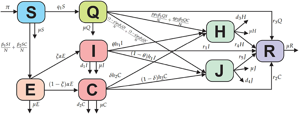
Figure 1. Compartmental diagram of the COVID-19 model with comorbidity.

Based on the compartmental diagram in Figure 1 and the model assumptions, we have the following system of differential equations:

$\begin{array}{l}\frac{dS}{dt}=\pi -\frac{{\beta }_{1}SI}{N}-\frac{{\beta }_{2}SC}{N}-q_{1}S-\mu S,\\ \frac{dE}{dt}=\frac{{\beta }_{1}SI}{N}+\frac{{\beta }_{2}SC}{N}-\alpha E-\mu E,\\ \frac{dI}{dt}=\xi \alpha E-h_{1}I-r_{1}I-d_{1}I-\mu I,\\ \frac{dC}{dt}=(1-\xi )\alpha E-h_{2}C-r_{2}C-d_{2}C-\mu C,\\ \frac{dQ}{dt}=q_{1}S-\frac{{\rho }_1{\beta }_{1}QI}{N}-\frac{{\rho }_2{\beta }_{2}QC}{N}-r_{3}Q-\mu Q,\\ \frac{dH}{dt}=\theta h_{1}I+\delta h_{2}C+\frac{p{\rho }_1{\beta }_{1}QI}{N}+\frac{q{\rho }_2{\beta }_{2}QC}{N}\\ -r_{4}H-d_{3}H-\mu H,\\ \frac{dJ}{dt}=(1-\theta )h_{1}I+(1-\delta )h_{2}C\\ +\frac{(1-p){\rho }_1{\beta }_{1}QI}{N}+\frac{(1-q){\rho }_2{\beta }_{2}QC}{N}-r_{5}J-d_{4}J-\mu J,\\ \frac{dR}{dt}=r_{1}I+r_{2}C+r_{3}Q+r_{4}H+r_{5}J-\mu R.& (1)\end{array}$

In this model, the COVID-19 model is divided into susceptible (S), exposed (E), infected without comorbidity (I), infected with comorbidity (C), isolated (Q), treatment isolated (H), isolated without treatment (J), and recovered (R). Susceptible subpopulation increases with the recruitment or birth rate denoted by π and can be infected due to contact with infected individuals without comorbidity and with comorbidity denoted by β₁ and β₂, respectively. Susceptible individuals who are quarantined are denoted by q₁ and cannot be returned to being susceptible due to the effects of public anxiety, which make some assumptions or opinions that susceptible individuals need to be quarantined, so that if quarantine is successful, then recovery is denoted by r₃ and if not successful due to contact with infected individuals without comorbidity and with comorbidity, showing symptoms of being infected, then isolation is denoted by ρ₁ and ρ₂, respectively. Furthermore, p and q are the proportion of changes from quarantine to isolation. The progression from exposed to infection is denoted α, and ξ is the proportion of change from exposed to infection without comorbidity. From the infected subpopulation without comorbidity and with comorbidity, isolation is denoted by h₁ and h₂. The parameters r₁, r₂, r₃, and r₄ indicate the recovery rate of the subpopulations infected without comorbidity, infected with comorbidity, quarantine, isolated with treatment, and isolated without treatment. Furthermore, deaths from each subpopulation are denoted by μ and deaths from COVID-19 in subpopulations I, C, H, and J are denoted by d₁, d₂, d₃, and d₄.

3. Mathematical analysis

3.1. Model validation

We calibrate our model (Equation 1) using cumulatively confirmed COVID-19 cases for Indonesia. We have retrieved COVID-19 case data from the Republic of Indonesia Task Force (SATGAS) situation report for the period 1 November 2020 to 19 May 2021 [9]. The parameter fitting uses the lsqcurvefit command, and the value of MAPE = 0.026022 is obtained. The results of the fitting parameters seem to match the infection case data as shown in Figure 2, and new parameter values are obtained according to conditions in Indonesia as follows in Table 1.

FIGURE 2

Figure 2. Parameter fitting results from the COVID-19 model.

TABLE 1

Table 1. Parameter values according to the fitting of the infected cases of COVID-19 in Indonesia.

3.2. Positivity and boundedness of solutions

The change in the total population is given by

$\begin{array}{l}\frac{dN}{dt}=\frac{dS}{dt}+\frac{dE}{dt}+\frac{dI}{dt}+\frac{dC}{dt}+\frac{dQ}{dt}+\frac{dH}{dt}+\frac{dJ}{dt}+\frac{dR}{dt},\\ =\pi -\mu N-d_{1}I-d_{2}C-d_{3}H-d_{4}J,\\ \le \pi -\mu N,\end{array}$

whose solutions give

$\begin{array}{l}N(t)\le \frac{\pi }{\mu }+\left(N(0)-\frac{\pi }{\mu }\right)e^{-\mu t}.\end{array}$

Consequently as t → ∞, then ${\text{lim}}_{t\to \infty }N(t)\le \frac{\pi }{\mu }$. So, we can conclude that N is boundedness to $N(t)\le \frac{\pi }{\mu }.$

Considering the above solutions, we have that the model has a boundedness solution which is contained in a feasible region Ω, where

$\begin{array}{l}\Omega =\left\{(S,E,I,C,Q,H,J,R)|N(t)\le \frac{\pi }{\mu }\right\}.\end{array}$

Next, we show the positivity of solving the Equation (1) system by following Riyapan et al. [42] and Rois et al. [46], as follows:

Theorem 1. Let S, E, I, C, Q, H, J, and R be the system solutions (Equation 1). If S(0) ≥ 0, E(0) ≥ 0, I(0) ≥ 0, C(0) ≥ 0, Q(0) ≥ 0, H(0) ≥ 0, J(0) ≥ 0, and R(0) ≥ 0, then all solutions are positive for every t ≥ 0.

Proof. 1. Take the first equation of the system (Equation 1) as follows:

$\begin{array}{l}\frac{dS}{dt}=\pi -\frac{{\beta }_{1}SI}{N}-\frac{{\beta }_{2}SC}{N}-q_{1}S-\mu S.\end{array}$

Let $\eta =\frac{{\beta }_{1}I}{N}+\frac{{\beta }_{2}C}{N}.$

$\begin{array}{l}\frac{dS}{dt}=\pi -S\left(\eta +q_1+\mu \right),\\ \frac{dS}{dt}+S\left(\eta +q_1+\mu \right)=\pi ,\\ \frac{d\left(e^{\left(q_1+\mu \right)t+{\int }_0^t\eta ds}S\left(t\right)\right)}{dt}=\pi e^{\left(q_1+\mu \right)t+{\int }_0^t\eta ds},& (2)\end{array}$

then a homogeneous solution is obtained

$\begin{array}{l}\frac{d(e^{(q_1+\mu )t+{\int }_0^t\eta ds}S(t))}{dt}=0,\\ S(t)=k{e}^{-(q_1+\mu )t-{\int }_0^t\eta ds}.\end{array}$

Thus, let us assume that the solution is non-homogeneous

$\begin{array}{ll}S(t)=k{e}^{-(q_1+\mu )t-{\int }_0^t\eta ds}.& (3)\end{array}$

Next, substituting the Equation (3) into the Equation (2) to get

$\begin{array}{l}\frac{dk(t)}{dt}=\pi e^{(q_1+\mu )t+{\int }_0^t\eta ds},\\ k(t)={\displaystyle {\int }_0^t}\pi e^{(q_1+\mu )y+{\int }_0^y\eta dx}dy+K.& (4)\end{array}$

The Equation (4) is substituted into the Equation (3), we get

$\begin{array}{l}S(t)={\displaystyle {\int }_0^t}\pi e^{(q_1+\mu )y+{\int }_0^y\eta dx}dy\times e^{-(q_1+\mu )t-{\int }_0^t\eta ds}\\ +S(0)e^{-(q_1+\mu )t-{\int }_0^t\eta ds}.\end{array}$

So, S(t) is positive for t ≥ 0.

2. Take the fifth equation of the system (Equation 1) as follows:

$\begin{array}{l}\frac{dQ}{dt}=q_{1}S-\frac{{\rho }_1{\beta }_{1}QI}{N}-\frac{{\rho }_2{\beta }_{2}QC}{N}-r_{3}Q-\mu Q.\end{array}$

Let $\omega =\frac{{{\rho }_1\beta }_{1}I}{N}+\frac{{{\rho }_2\beta }_{2}C}{N}.$

$\begin{array}{l}\frac{dQ}{dt}=q_{1}S-Q(\omega +r_3+\mu ),\\ \frac{dQ}{dt}+Q(\omega +r_3+\mu )=q_{1}S,\\ \frac{d\left(e^{(r_3+\mu )t+{\int }_0^t\omega ds}Q(t)\right)}{dt}=q_{1}S{e}^{(r_3+\mu )t+{\int }_0^t\omega ds},& (5)\end{array}$

then a homogeneous solution is obtained

$\begin{array}{l}\frac{d\left(e^{(r_3+\mu )t+{\int }_0^t\omega ds}Q(t)\right)}{dt}=0,\\ Q(t)=k{e}^{-(r_3+\mu )t-{\int }_0^t\omega ds}.\end{array}$

Thus, let us assume that the solution is non-homogeneous

$\begin{array}{ll}Q(t)=k{e}^{-(r_3+\mu )t-{\int }_0^t\omega ds}.& (6)\end{array}$

Next, substituting the Equation (6) into the Equation (5) to get

$\begin{array}{l}\frac{dk(t)}{dt}=q_{1}S{e}^{(r_3+\mu )t+{\int }_0^t\omega ds},\\ k(t)={\displaystyle {\int }_0^t}{q}_{1}S{e}^{(r_3+\mu )y+{\int }_0^y\omega dx}dy+K.& (7)\end{array}$

The the Equation (7) is substituted into the Equation (6), we get

$\begin{array}{l}Q(t)={\displaystyle {\int }_0^t}{q}_{1}S{e}^{(r_3+\mu )y+{\int }_0^y\omega dx}dy\times e^{-(r_3+\mu )t-{\int }_0^t\omega ds}\\ +Q(0)e^{-(r_3+\mu )t-{\int }_0^t\omega ds}.\end{array}$

So, Q(t) is positive for t ≥ 0.

3. Take the second equation of the system (Equation 1) as follows:

$\begin{array}{l}\frac{dE}{dt}=\frac{{\beta }_{1}SI}{N}+\frac{{\beta }_{2}SC}{N}-\alpha E-\mu E\ge -\alpha E-\mu E,\end{array}$

or

$\begin{array}{l}\frac{dE(t)}{dt}\ge -E(\alpha +\mu ),\\ {\displaystyle \int }\frac{dE(t)}{E}\ge {\displaystyle \int }-(\alpha +\mu )dt,\\ E(t)\ge e^{-(\alpha +\mu )t+k},\\ E(t)\ge E(0)e^{-(\alpha +\mu )t}.\end{array}$

Thus, E(t) is positive for t ≥ 0. Furthermore, in the same way as proof number 3, I(t), C(t), H(t), J(t), and R(t) can be shown respectively to be positive.□

3.3. Equilibrium point and basic reproduction number

The equilibrium point of the system (Equation 1) is obtained by setting the right-hand side to zeros. Therefore, the first equilibrium point is obtained, namely the disease-free equilibrium point, as follows:

$\begin{array}{l}{X}^0=\left(S^0,E^0,I^0,C^0,Q^0,H^0,J^0,R^0\right)\\ =\left(\frac{\pi }{a_1},0,0,0,\frac{\pi q_1}{a_1{a}_5},0,0,\frac{\pi q_1{r}_3}{a_1{a}_5\mu }\right).\end{array}$

Where a₁ = q₁ + μ and a₅ = r₃ + μ.

Furthermore, the basic reproduction number, denoted by R₀, is obtained using the next-generation matrix method [55, 56]. The constituent components of the next-generation matrix method only consist of infected subpopulation groups, namely:

$\begin{array}{l}f=\left[\begin{array}{c}\frac{{\beta }_{1}SI}{N}+\frac{{\beta }_{2}SC}{N}\\ 0\\ 0\end{array}\right],\text{ and }v=\left[\begin{array}{c}{a}_{2}E\\ -\xi \alpha E+a_{3}I\\ -(1-\xi )\alpha E+a_{4}C\end{array}\right].\end{array}$

The partial derivative evaluated at X⁰ gives

$\begin{array}{l}F\left(X^0\right)=\left[\begin{array}{ccc}0& \frac{{\beta }_1{a}_5\mu }{(a_5\mu +q_1\mu +q_1{r}_3)}& \frac{{\beta }_2{a}_5\mu }{(a_5\mu +q_1\mu +q_1{r}_3)}\\ 0& 0& 0\\ 0& 0& 0\end{array}\right]\\ \text{and }V\left(X^0\right)=\left[\begin{array}{ccc}{a}_2& 0& 0\\ -\xi \alpha & a_3& 0\\ -(1-\xi )\alpha & 0& a_4\end{array}\right].\end{array}$

The inverse of the V(X⁰) matrix is

$\begin{array}{l}{V}^{-1}=\left[\begin{array}{ccc}\frac{1}{a_2}& 0& 0\\ \frac{\xi \alpha }{a_2{a}_3}& \frac{1}{a_3}& 0\\ \frac{(1-\xi )\alpha }{a_2{a}_4}& 0& \frac{1}{a_4}\end{array}\right].\end{array}$

Based on the F(X⁰) and V⁻¹(X⁰) matrices, the next-generation matrix FV⁻¹ can be formed so that we can obtain

$\begin{array}{l}F{V}^{-1}=\left[\begin{array}{ccc}\frac{{\beta }_1{a}_5\mu \xi \alpha }{a_2{a}_3(a_5\mu +q_1\mu +q_1{r}_3)}+\frac{{\beta }_2{a}_5\mu \alpha (1-\xi )}{a_2{a}_4(a_5\mu +q_1\mu +q_1{r}_3)}& \frac{{\beta }_1{a}_5\mu }{a_3(a_5\mu +q_1\mu +q_1{r}_3)}& \frac{{\beta }_1{a}_5\mu }{a_4(a_5\mu +q_1\mu +q_1{r}_3)}\\ 0& 0& 0\\ 0& 0& 0\end{array}\right].\end{array}$

So, the basic reproduction number is obtained based on the eigenvalues of the FV⁻¹ matrix as follows:

$\begin{array}{l}{R}_0=\rho (M)=\frac{a_5\mu \alpha ({\beta }_1\xi a_4+{\beta }_2{a}_3(1-\xi ))}{a_2{a}_3{a}_4(a_5\mu +q_1\mu +q_1{r}_3)}.\end{array}$

Next, the second equilibrium point is obtained, namely the endemic equilibrium point X^* = (S^*, E^*, I^*, C^*, Q^*, H^*, J^*, R^*) with

$\begin{array}{l}{S}^{*}=\frac{\pi a_5}{A_1{R}_0},\\ E^{*}=\frac{\pi }{a_2{R}_0}(R_0-1),\\ I^{*}=\frac{\pi \xi \alpha }{a_2{a}_3{R}_0}(R_0-1),\\ C^{*}=\frac{(1-\xi )\pi \alpha }{a_2{a}_4{R}_0}(R_0-1),\\ Q^{*}=\frac{a_2{a}_3{a}_4{a}_5{q}_1\pi }{A_3},\\ H^{*}=(R_0-1)A_4,\\ J^{*}=(R_0-1)A_5,\\ R^{*}=(R_0-1)A_6+\frac{r_3{a}_2{a}_3{a}_4{a}_5{q}_1\pi }{\mu A_3},\end{array}$

with A₁ = a₅μ + μq₁ + q₁r₃, A₂ = ρ₁β₁a₄μαξ + ρ₂β₂a₃μα(1 − ξ), A₃ = A₁A₂(R₀ − 1) + a₂a₃a₄a₅A₁R₀, $A_4=\frac{\pi \alpha }{a_6{R}_0}\left(\frac{\theta h_1\xi }{a_2{a}_3}+\frac{\delta h_2(1-\xi )}{a_2{a}_4}+\frac{p{\rho }_1{\beta }_1{q}_1{a}_4{a}_5\mu \xi }{A_3}+\frac{q{\rho }_2{\beta }_2{q}_1{a}_3{a}_5\mu (1-\xi )}{A_3}\right)$, $A_5=\frac{\pi \alpha }{a_7{R}_0}(\frac{(1-\theta )h_1\xi }{a_2{a}_3}+\frac{(1-\delta )h_2(1-\xi )}{a_2{a}_4}+\frac{(1-p){\rho }_1{\beta }_1\mu \xi a_4{a}_5{q}_1}{A_3}+\frac{(1-q){\rho }_2{\beta }_2\mu a_3{a}_5{q}_1(1-\xi )}{A_3})$, and $A_6=\frac{r_1\pi \alpha \xi }{\mu a_2{a}_3{R}_0}+\frac{r_2\pi \alpha (1-\xi )}{\mu a_2{a}_4{R}_0}+\frac{r_4{A}_4}{\mu }+\frac{r_5{A}_5}{\mu }$.

The existence of the endemic equilibrium point X^* depends on the value of R₀. If the value of R₀ < 1 is taken, then the endemic equilibrium point X^* does not exist because it is clear that E^*, I^*, C^*, H^*, and J^* are obtained negative. If R₀ = 1, then we get the equilibrium point X^* = X⁰, which causes the equilibrium point X^* not to exist. Furthermore, if R₀ > 1, then we get S^*, E^*, I^*, C^*, Q^*, H^*, J^*, and R^* are positive and the endemic equilibrium point X^* exists.

3.4. Local stability

The local stability of the equilibrium point is obtained by linearizing system (Equation 1), which yields the following jacobian matrix below:

$\begin{array}{ll}J=\left[\begin{array}{cccccccc}{B}_1-B_2-a_1& B_1& B_1-\frac{{\beta }_{1}S}{N}& B_1-\frac{{\beta }_{2}S}{N}& B_1& B_1& B_1& B_1\\ B_2-B_1& -B_2-a_2& \frac{{\beta }_{1}S}{N}-B_1& \frac{{\beta }_{2}S}{N}-B_1& -B_1& -B_1& -B_1& -B_1\\ 0& \xi \alpha & -a_3& 0& 0& 0& 0& 0\\ 0& (1-\xi )\alpha & 0& -a_4& 0& 0& 0& 0\\ q_1+B_3& B_3& B_3-\frac{{\rho }_1{\beta }_{1}Q}{N}& B_3-\frac{{\rho }_2{\beta }_{2}Q}{N}& B_3-B_4-a_5& B_3& B_3& B_3\\ -B_5& -B_5& B_6-B_5& B_7-B_5& B_8-B_5& -B_5-a_6& -B_5& -B_5\\ -B_9& -B_9& B_{10}-B_9& B_{11}-B_9& B_{12}-B_9& -B_9& -B_9-a_7& -B_9\\ 0& 0& r_1& r_2& r_3& r_4& r_5& -\mu \end{array}\right]& (8)\end{array}$

With $B_1=\frac{{\beta }_{1}SI}{N^2}+\frac{{\beta }_{2}SC}{N^2}$, $B_2=\frac{{\beta }_{1}I}{N}+\frac{{\beta }_{2}C}{N}$, $B_3=\frac{{\rho }_1{\beta }_{1}QI}{N^2}+\frac{{\rho }_2{\beta }_{2}QC}{N^2}$, $\$B_4=\frac{{\rho }_1{\beta }_{1}I}{N}+\frac{{\rho }_2{\beta }_{2}C}{N}$, $B_5=\frac{p{\rho }_1{\beta }_{1}QI}{N^2}+\frac{q{\rho }_2{\beta }_{2}QC}{N^2}$, $B_6=\theta h_1+\frac{p{\rho }_1{\beta }_{1}Q}{N}$, $B_7=\delta h_2+\frac{q{\rho }_2{\beta }_{2}Q}{N}$, $B_8=\frac{p{\rho }_1{\beta }_{1}I}{N}+\frac{q{\rho }_2{\beta }_{2}C}{N}$, $B_9=\frac{(1-p){\rho }_1{\beta }_{1}QI}{N^2}+\frac{(1-q){\rho }_2{\beta }_{2}QC}{N^2}$, $B_{10}=(1-\theta )h_1+\frac{(1-p){\rho }_1{\beta }_{1}Q}{N}$, $B_{11}=(1-\delta )h_2+\frac{(1-q){\rho }_2{\beta }_{2}Q}{N}$, and $B_{12}=\frac{(1-p){\rho }_1{\beta }_{1}I}{N}+\frac{(1-q){\rho }_2{\beta }_{2}C}{N}.$

3.4.1. Local stability of disease-free equilibrium point

Evaluating (8) at X⁰ yields

$\begin{array}{l}J(X^0)=\left[\begin{array}{cccccccc}-a_1& 0& -{\beta }_1{C}_1& -{\beta }_2{C}_1& 0& 0& 0& 0\\ 0& -a_2& {\beta }_1{C}_1& {\beta }_2{C}_1& 0& 0& 0& 0\\ 0& \xi \alpha & -a_3& 0& 0& 0& 0& 0\\ 0& (1-\xi )\alpha & 0& -a_4& 0& 0& 0& 0\\ q_1& 0& -{\rho }_1{\beta }_1{C}_2& -{\rho }_2{\beta }_2{C}_2& -a_5& 0& 0& 0\\ 0& 0& \theta h_1+p{\rho }_1{\beta }_1{C}_2& \delta h_2+q{\rho }_2{\beta }_2{C}_2& 0& -a_6& 0& 0\\ 0& 0& (1-\theta )h_1+(1-p){\rho }_1{\beta }_1{C}_2& (1-\delta )h_2+(1-q){\rho }_2{\beta }_2{C}_2& 0& 0& -a_7& 0\\ 0& 0& r_1& r_2& r_3& r_4& r_5& -\mu \end{array}\right],\end{array}$

With $C_1=\frac{a_5\mu }{(a_5+q_1)\mu +q_1{r}_3}$ and $C_2=\frac{q_1\mu }{(a_5+q_1)\mu +q_1{r}_3}.$ The characteristic equation for the |J(X⁰) − λI| = 0 is as follows:

$\begin{array}{l}(-a_1-\lambda )(-a_5-\lambda )(-a_6-\lambda )(-a_7-\lambda )(-\mu -\lambda )\\ \left|\begin{array}{ccc}-a_2-\lambda & {\beta }_1{C}_1& {\beta }_2{C}_1\\ \xi \alpha & -a_3-\lambda & 0\\ (1-\xi )\alpha & 0& -a_4-\lambda \end{array}\right|=0.& (9)\end{array}$

Based on the Equation (9), we obtain the eigenvalues λ₁ = λ₂ = λ₃ = λ₄ = λ₅ < 0. Therefore, the stability of the disease-free equilibrium point depends on

$\begin{array}{ll}{M}_1=\left|\begin{array}{ccc}-a_2-\lambda & {\beta }_1{C}_1& {\beta }_2{C}_1\\ \xi \alpha & -a_3-\lambda & 0\\ (1-\xi )\alpha & 0& -a_4-\lambda \end{array}\right|.& (10)\end{array}$

From the Equation (10), we obtain the following characteristic equation:

$\begin{array}{ll}{\lambda }^3+k_1{\lambda }^2+k_2\lambda +k_3=0,& (11)\end{array}$

with

$\begin{array}{l}{k}_1=a_2+a_3+a_4,\\ k_2=a_2{a}_3(1-R_0)+a_2{a}_4(1-R_0)\\ +a_3{a}_4+\frac{a_4{\beta }_1\alpha C_1\xi }{a_3}+\frac{a_3{\beta }_2\alpha C_1(1-\xi )}{a_4},\text{ and}\\ k_3=a_2{a}_3{a}_4(1-R_0).\end{array}$

In the Equation (11), it is clear that k₁ > 0, and if R₀ < 1, then k₂ > 0 and k₃ > 0. Therefore, the stability property of the equilibrium point X⁰ is established using the Routh–Hurwitz criterion. Furthermore, the equilibrium point X⁰ is asymptotically stable if and only if it satisfies the following criteria:

1. k₁ > 0,

2. k₃ > 0, and

3. k₁k₂ − k₃ > 0.

Criteria Equations (1) and (2) have been met so that the disease-free equilibrium point X⁰ is locally asymptotically stable if it meets k₁k₂ − k₃ > 0 where

$\begin{array}{l}{k}_1{k}_2-k_3>0,\\ (a_2+a_3+a_4)\\ \left(a_2{a}_4(1-R_0)+a_3{a}_4+\frac{a_4{\beta }_1\alpha C_1\xi }{a_3}+\frac{a_3{\beta }_2\alpha C_1(1-\xi )}{a_4}\right)\\ +a_2^2{a}_3(1-R_0)+a_2{a}_3^2(1-R_0)>0.\end{array}$

It is clear that the Routh–Hurwitz criteria are satisfied; thus, the roots of the characteristic Equation (11) have negative real parts. Therefore, the disease-free equilibrium point is asymptotically locally stable if R₀ < 1.

3.4.2. Local stability of the endemic equilibrium point

Evaluating (8) at X^* yields

$\begin{array}{l}J(X^{*})=\left[\begin{array}{cccccccc}{B}_1-B_{13}& B_1& B_1-\frac{{\beta }_1{S}^{*}}{N}& B_1-\frac{{\beta }_2{S}^{*}}{N}& B_1& B_1& B_1& B_1\\ B_2-B_1& -B_{14}& \frac{{\beta }_1{S}^{*}}{N}-B_1& \frac{{\beta }_2{S}^{*}}{N}-B_1& -B_1& -B_1& -B_1& -B_1\\ 0& \xi \alpha & -a_3& 0& 0& 0& 0& 0\\ 0& (1-\xi )\alpha & 0& -a_4& 0& 0& 0& 0\\ q_1+B_3& B_3& B_3-\frac{{\rho }_1{\beta }_1{Q}^{*}}{N}& B_3-\frac{{\rho }_2{\beta }_2{Q}^{*}}{N}& B_3-B_{15}& B_3& B_3& B_3\\ -B_5& -B_5& B_6-B_5& B_7-B_5& B_8-B_5& -B_{16}& -B_5& -B_5\\ -B_9& -B_9& B_{10}-B_9& B_{11}-B_9& B_{12}-B_9& -B_9& -B_{17}& -B_9\\ 0& 0& r_1& r_2& r_3& r_4& r_5& -\mu \end{array}\right],\end{array}$

With $B_1=\frac{{\beta }_1{S}^{*}{I}^{*}}{N^2}+\frac{{\beta }_2{S}^{*}{C}^{*}}{N^2}$, $B_2=\frac{{\beta }_1{I}^{*}}{N}+\frac{{\beta }_2{C}^{*}}{N}$, $B_3=\frac{{\rho }_1{\beta }_1{Q}^{*}{I}^{*}}{N^2}+\frac{{\rho }_2{\beta }_2{Q}^{*}{C}^{*}}{N^2}$, $B_4=\frac{{\rho }_1{\beta }_1{I}^{*}}{N}+\frac{{\rho }_2{\beta }_2{C}^{*}}{N}$, $B_5=\frac{p{\rho }_1{\beta }_1{Q}^{*}{I}^{*}}{N^2}+\frac{q{\rho }_2{\beta }_2{Q}^{*}{C}^{*}}{N^2}$, $B_6=\theta h_1+\frac{p{\rho }_1{\beta }_1{Q}^{*}}{N}$, $B_7=\delta h_2+\frac{q{\rho }_2{\beta }_2{Q}^{*}}{N}$, $B_8=\frac{p{\rho }_1{\beta }_1{I}^{*}}{N}+\frac{q{\rho }_2{\beta }_2{C}^{*}}{N}$, $B_9=\frac{(1-p){\rho }_1{\beta }_1{Q}^{*}{I}^{*}}{N^2}+\frac{(1-q){\rho }_2{\beta }_2{Q}^{*}{C}^{*}}{N^2}$, $B_{10}=(1-\theta )h_1+\frac{(1-p){\rho }_1{\beta }_1{Q}^{*}}{N}$, $B_{11}=(1-\delta )h_2+\frac{(1-q){\rho }_2{\beta }_2{Q}^{*}}{N}$, $B_{12}=\frac{(1-p){\rho }_1{\beta }_{1}I}{N}+\frac{(1-q){\rho }_2{\beta }_{2}C}{N}$, B₁₃ = B₂ + a₁, B₁₄ = B₂ + a₂, B₁₅ = B₄ + a₅, B₁₆ = B₅ + a₆, and B₁₇ = B₉ + a₇.

The characteristic equation of the |J(X^*) − λI| = 0 is

$\begin{array}{l}{\lambda }^8+k_1{\lambda }^7+k_2{\lambda }^6+k_3{\lambda }^5+k_4{\lambda }^4+k_5{\lambda }^3+k_6{\lambda }^2+k_7\lambda \\ +k_8=0,& (12)\end{array}$

It is difficult to prove analytically that all eigenvalues of J have negative real parts for R₀ > 1. However, from our numerical simulations (case R₀ > 1), all eigenvalues have negative real parts.

Figure 3 gives the projection of three orbits of three different initial conditions when R₀ > 1 on the I − C plane. The component (I, C) of the equilibrium X^* is not (0, 0). This simulation indicates that the endemic equilibrium X^* is locally asymptotically stable when R₀ > 1.

FIGURE 3

Figure 3. Projection of three orbits of the model on the I − C plane.

3.5. Global stability analysis

In this study, we prove the global stability of disease-free and endemic equilibrium points by constructing the suitable Lyapunov function and following the theorem from Alligood et al. [57].

3.5.1. Global stability of the disease-free equilibrium point

Theorem 2. Disease-free equilibrium point X⁰ is globally asymptotically stable if R₀ < 1 and unstable if R₀ > 1.

Proof. Defined Lyapunov function

$\begin{array}{ll}L={\kappa }_{1}E+{\kappa }_{2}I+{\kappa }_{3}C,& (13)\end{array}$

where

$\begin{array}{l}{\kappa }_1=a_1{a}_2{a}_3{a}_4,\\ {\kappa }_2=\frac{\pi {\beta }_1{a}_2{a}_4}{N},\text{and}\\ {\kappa }_3=\frac{\pi {\beta }_2{a}_2{a}_3}{N}.\end{array}$

The function L needs to be proven to determine whether Lyapunov is strong or weak for X⁰.

$\begin{array}{l}L\left({\vec{x}}^{*}\right)=L\left(S^0,E^0,I^0,C^0,Q^0,H^0,J^0,R^0\right),\\ L\left({\vec{x}}^{*}\right)={\kappa }_1{E}^0+{\kappa }_2{I}^0+{\kappa }_3{C}^0=0.\end{array}$

It is proven that $L\left({\vec{x}}^{*}\right)=0.$ Next,

$\begin{array}{l}L\left(\vec{x}\right)={\kappa }_{1}E+{\kappa }_{2}I+{\kappa }_{3}C,\end{array}$

Because ∀(S, E, I, C, Q, H, J, R) ≠ (S⁰, E⁰, I⁰, C⁰, Q⁰, H⁰, J⁰, R⁰), so it is proved that $L\left(\vec{x}\right)>0$.

Thus, the Equation (13) can be reduced to

$\begin{array}{l}\frac{\partial L}{\partial t}={\kappa }_1\frac{dE}{dt}+{\kappa }_2\frac{dI}{dt}+{\kappa }_3\frac{dC}{dt}\\ ={\kappa }_1\left(\frac{{\beta }_{1}SI+{\beta }_{2}SC}{N}-a_{2}E\right)\\ +{\kappa }_2(\xi \alpha E-a_{3}I)+{\kappa }_3((1-\xi )\alpha E-a_{4}C),\end{array}$

so, we obtain

$\begin{array}{l}=a_1{a}_2{a}_3{a}_4(\frac{{\beta }_{1}SI+{\beta }_{2}SC}{N}-a_{2}E+\frac{\pi {\beta }_1{a}_2{a}_4\xi \alpha E}{a_1{a}_2{a}_3{a}_{4}N}\\ +\frac{\pi {\beta }_2{a}_2{a}_3(1-\xi )\alpha E}{a_1{a}_2{a}_3{a}_{4}N}-\frac{\pi {\beta }_{1}I}{a_{1}N}-\frac{\pi {\beta }_{2}C}{a_{1}N}).\end{array}$

Let $S=\frac{\pi }{a_1}$, so we get

$\begin{array}{l}\frac{\partial L}{\partial t}=a_1{a}_2^2{a}_3{a}_{4}E(R_0-1).\end{array}$

Based on the description above, it can be concluded that $\frac{\partial L}{\partial t}<0$ if R₀ < 1 and $\frac{\partial L}{\partial t}=0$ if E = 0. Hence, by Lasalle's invariance principle, the disease-free equilibrium point in the spread of COVID-19 (X⁰) is globally asymptotically stable if R₀ < 1.□

3.5.2. Global stability of the endemic equilibrium point

Theorem 3. If R₀ > 1, then the endemic equilibrium point X^* is said to be globally asymptotically stable.

Proof. The Lyapunov function is defined as follows:

$\begin{array}{ll}L=\frac{1}{2}{\left[S_S+E_E+I_I+C_C+Q_Q+H_H+J_J+R_R\right]}^2,& (14)\end{array}$

Where $S_S=\left(S-S^{*}\right)$, $E_E=\left(E-E^{*}\right)$, $I_I=\left(I-I^{*}\right)$, $C_C=\left(C-C^{*}\right)$, $Q_Q=\left(Q-Q^{*}\right)$, $H_H=\left(H-H^{*}\right)$, $J_J=\left(J-J^{*}\right)$, and dan $R_R=\left(R-R^{*}\right)$.

The function L needs to be proven to determine whether the Lyapunov function is strong or weak for X^*.

$\begin{array}{l}L\left({\vec{x}}^{*}\right)=L\left(S^{*},E^{*},I^{*},C^{*},Q^{*},H^{*},J^{*},R^{*}\right),\\ L\left({\vec{x}}^{*}\right)=\frac{1}{2}{\left[S_S^{*}+E_E^{*}+I_I^{*}+C_C^{*}+Q_Q^{*}+H_H^{*}+J_J^{*}+R_R^{*}\right]}^2\\ =0.\end{array}$

Where $S_S^{*}=(S^{*}-S^{*})$, $E_E^{*}=(E^{*}-E^{*})$, $I_I^{*}=(I^{*}-I^{*})$, $C_C^{*}=(C^{*}-C^{*})$, $Q_Q^{*}=(Q^{*}-Q^{*})$, $H_H^{*}=(H^{*}-H^{*})$, $J_J^{*}=(J^{*}-J^{*})$, and $R_R^{*}=(R^{*}-R^{*})$. It is proven that $L\left({\vec{x}}^{*}\right)=0.$

Next,

$\begin{array}{l}L(\vec{x})=\frac{1}{2}{\left[S_S+E_E+I_I+C_C+Q_Q+H_H+J_J+R_R\right]}^2.\end{array}$

Because ∀(S, E, I, C, Q, H, J, R) ≠ (S⁰, E⁰, I⁰, C⁰, Q⁰, H⁰, J⁰, R⁰), so that it is proven that $L(\vec{x})>0$. Next, we check that the Equation (14) is reduced to

$\begin{array}{l}\frac{\partial L}{\partial t}=\left[S_S+E_E+I_I+C_C+Q_Q+H_H+J_J+R_R\right]\\ \frac{d}{dt}\left[S+E+I+C+Q+H+J+R\right],\\ =\left[S_S+E_E+I_I+C_C+Q_Q+H_H+J_J+R_R\right]\\ [\pi -\mu (S+E+I+C+Q+H+J+R)\\ -d_{1}I-d_{2}C-d_{3}H-d_{4}J],\end{array}$

Let $\pi =\mu (S^{*}+E^{*}+I^{*}+C^{*}+Q^{*}+H^{*}+J^{*}+R^{*})+d_1{I}^{*}+d_2{C}^{*}+d_3{H}^{*}+d_4{J}^{*}.$ So that it gives

$\begin{array}{l}=\left[S_S+E_E+I_I+C_C+Q_Q+H_H+J_J+R_R\right]\\ \times [-[\mu (S_S+E_E+I_I+C_C+Q_Q+H_H+J_J+R_R)+d_1(I-I^{*})\\ +d_2(C-C^{*})+d_3(H-H^{*})+d_4(J-J^{*})]],\\ =-\left[S_S+E_E+I_I+C_C+Q_Q+H_H+J_J+R_R\right]\\ \times [\mu (S_S+E_E+I_I+C_C+Q_Q+H_H+J_J+R_R)+d_1(I-I^{*})\\ +d_2(C-C^{*})+d_3(H-H^{*})+d_4(J-J^{*})]].\end{array}$

Based on the description above, it can be concluded that $\frac{\partial L}{\partial t}<0$ if R₀ > 1 and $\frac{\partial L}{\partial t}=0$ if S = S^*, E = E^*, I = I^*, C = C^*, Q = Q^*, H = H^*, J = J^*, and R = R^*. Hence, by Lasalle's invariance principle, it means that the endemic equilibrium point in the spread of COVID-19 (X^*) is globally asymptotically stable if R₀ > 1.□

The terms of existence and the type of stability of the equilibrium point of the system of equations are summarized in Table 2.

TABLE 2

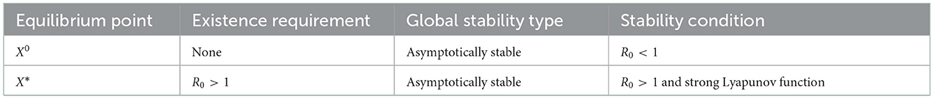
Table 2. Stability conditions.

3.6. Sensitivity analysis

The sensitivity analysis aims to determine the parameters that cause the spread of the COVID-19 virus. The sensitivity index of the basic reproduction number depends on the differentiation of the parameters contained in the basic reproduction number [58, 59]. Sensitivity index R₀ to the parameters is as follows:

$\begin{array}{l}{I}_{\alpha }^{R_0}=\frac{\partial R_0}{\partial \alpha }\frac{\alpha }{R_0}=\frac{\mu }{\alpha +\mu },\\ I_{{\beta }_1}^{R_0}=\frac{\partial R_0}{\partial {\beta }_1}\frac{{\beta }_1}{R_0}=\frac{{\beta }_1\xi a_4}{{\beta }_1\xi a_4+{\beta }_2{a}_3(1-\xi )},\\ I_{{\beta }_2}^{R_0}=\frac{\partial R_0}{\partial {\beta }_2}\frac{{\beta }_2}{R_0}=\frac{{\beta }_2{a}_3(1-\xi )}{{\beta }_1\xi a_4+{\beta }_2{a}_3(1-\xi )},\\ I_{\xi }^{R_0}=\frac{\partial R_0}{\partial \xi }\frac{\xi }{R_0}=\frac{{\beta }_1\xi a_4-{\beta }_2\xi a_3}{{\beta }_1\xi a_4+{\beta }_2{a}_3(1-\xi )},\\ I_{q_1}^{R_0}=\frac{\partial R_0}{\partial q_1}\frac{q_1}{R_0}=-\frac{q_1}{q_1+\mu },\\ I_{h_1}^{R_0}=\frac{\partial R_0}{\partial h_1}\frac{h_1}{R_0}=\frac{a_4{\beta }_1{h}_1\xi }{-a_3({\beta }_2{a}_3(1-\xi )+{\beta }_1{a}_4\xi )},\\ I_{r_1}^{R_0}=\frac{\partial R_0}{\partial r_1}\frac{r_1}{R_0}=\frac{{\beta }_1{r}_1{a}_4\xi }{-a_3({\beta }_2{a}_3(1-\xi )+{\beta }_1{a}_4\xi )},\\ I_{d_1}^{R_0}=\frac{\partial R_0}{\partial d_1}\frac{d_1}{R_0}=\frac{{\beta }_1{d}_1{a}_4\xi }{-a_3({\beta }_2{a}_3(1-\xi )+{\beta }_1{a}_4\xi )},\\ I_{h_2}^{R_0}=\frac{\partial R_0}{\partial h_2}\frac{h_2}{R_0}=\frac{{\beta }_2{h}_2{a}_3(1-\xi )}{-a_4({\beta }_2{a}_3(1-\xi )+{\beta }_1{a}_4\xi )},\\ I_{r_2}^{R_0}=\frac{\partial R_0}{\partial r_2}\frac{r_2}{R_0}=\frac{{\beta }_2{r}_2{a}_3(1-\xi )}{-a_4({\beta }_2{a}_3(1-\xi )+{\beta }_1{a}_4\xi )},\\ I_{d_2}^{R_0}=\frac{\partial R_0}{\partial d_2}\frac{d_2}{R_0}=\frac{{\beta }_2{r}_2{a}_3(1-\xi )}{-a_4({\beta }_2{a}_3(1-\xi )+{\beta }_1{a}_4\xi )},\\ I_{\mu }^{R_0}=\frac{\partial R_0}{\partial \mu }\frac{\mu }{R_0}=\frac{-(\alpha ((-2\xi +2){\beta }_2+2{\beta }_1\xi ){\mu }^5+a_8(1-\xi ){\beta }_2+{\beta }_1{a}_9\xi ){\mu }^4+2a_{10}((1-\xi )a_3{\beta }_2+{\beta }_1\xi a_4){\mu }^3}{a_1^2{a}_2^2{a}_3^2{a}_4^2}\\ -\frac{(((-a_{12})q_1+a_{11}^2)\alpha +a_{11}^2(a_{12}+q_1)(\xi -1){\beta }_2-(((a_{11})q_1-a_{12}^2)\alpha -a_{12}^2(a_{11}+q_1)){\beta }_1\xi ){\mu }^2}{a_1^2{a}_2^2{a}_3^2{a}_4^2}\\ -\frac{2(a_{11}\alpha q_1({\beta }_1\xi +{\beta }_2(1-\xi ))a_{11}\mu +a_{12}\alpha ((\xi -1)a_{11}{\beta }_2-{\beta }_1\xi a_{12})q_1{a}_{11})}{a_1^2{a}_2^2{a}_3^2{a}_4^2},\end{array}$

With a₈ = (4d₁ + α + d₂ + h₁ + h₂ + q₁ + 4r₁ + r₂), a₉ = d₁ + α + 4d₂ + h₁ + 4h₂ + q₁ + r₁ + 4r₂, a₁₀ = (d₁ + α + d₂ + h₁ + h₂ + q₁ + r₁ + r₂), a₁₁ = h₁ + r₁ + d₁, and a₁₂ = h₂ + r₂ + d₂.

The parameter sensitivity index is shown in Table 3.

TABLE 3

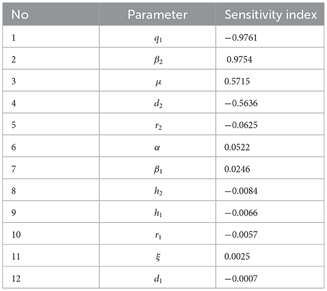
Table 3. Sensitivity analysis.

From Table 3, we can see that the most sensitive parameters are q₁ and β₂. A positive index means that if we reduce the parameter by almost 10%, then the value of the basic reproduction number can decrease by 10%.

4. Simulation of the model without control

This section presents a numerical solution of system (1) using the Fourth-order Runge–Kutta method. The parameter values used in this simulation are shown in Table 1 and three different initial values. In this simulation, the stability of the disease-free equilibrium point is shown from the parameter values given in Table 1, except for the parameter q₁ = 0.56574, the value is R₀ = 0.456 < 1. Based on the value of these parameters, the disease-free equilibrium point is obtained, namely X⁰ = (6527542, 0, 0, 0, 83496205, 0, 0, 183499868).

Next, the graph of the solution R₀ < 1 is obtained in Figure 4.

FIGURE 4

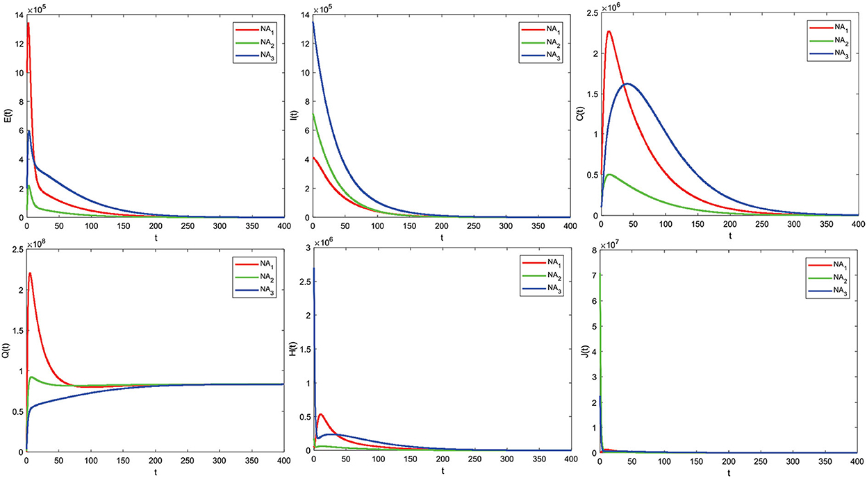
Figure 4. COVID-19 model solution graph for R₀ < 1.

The analysis results from 3.4.1, and Theorem 2 are illustrated numerically. Numerical simulations with some initial values show that the graph solution is toward and close to the disease-free equilibrium point X⁰ (converging toward the disease-free equilibrium point X₀). Based on the graph, this means that after all this time, no individual has been infected with COVID-19. The numerical results support the analysis that if R₀ < 1, then the disease-free equilibrium point X⁰ is asymptotically stable locally and globally given different initial values.

We show the stability of the endemic equilibrium point, the parameter values in Table 1 are used, and three different values, so we get R₀ = 1.47 > 1. Similarly, the disease-free equilibrium point is obtained

$X^0=(21071493,0,0,0,79018695,0,0,174052991)$

and the endemic equilibrium point is given as

$\begin{array}{l}{X}^{*}=(S^{*},E^{*},I^{*},C^{*},Q^{*},H^{*},J^{*},R^{*}),\\ =(6031017,10196616,1933377,63222893,\\ 2119885,362896,798735,30671327).\end{array}$

The solution graph for the case of R₀ > 1 is obtained as follows in Figure 5.

FIGURE 5

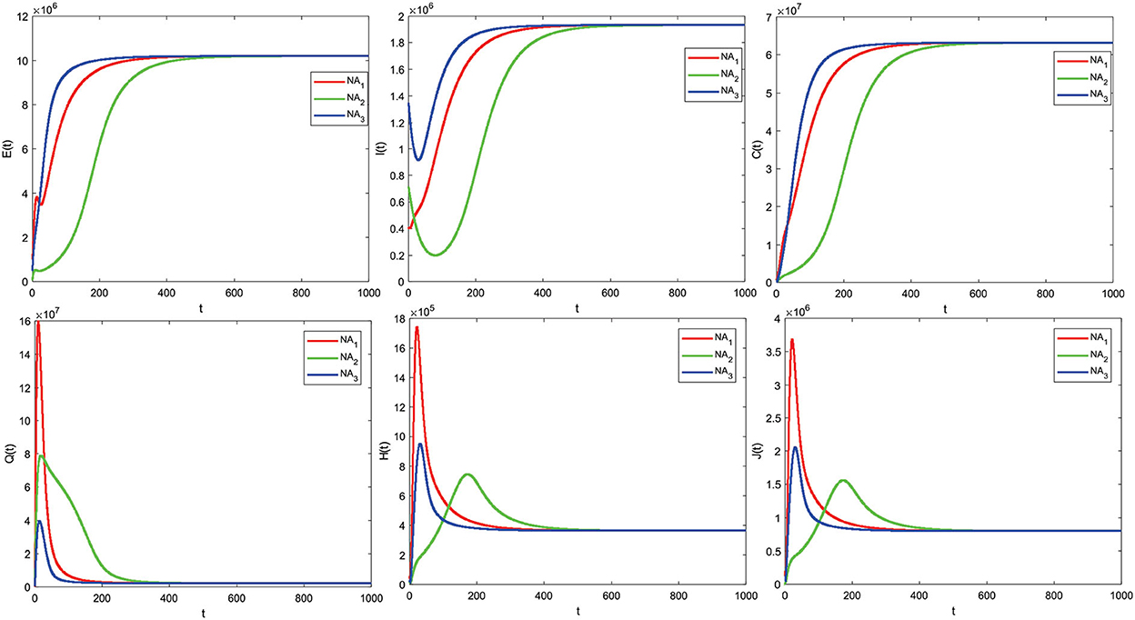
Figure 5. The COVID-19 model solution graph for R₀ > 1.

The numerical simulation results support the analysis from 3.4.2 and Theorem 3 that some of the initial values given are obtained by the graph of the solution leading to the endemic equilibrium point X^* (converging to the endemic equilibrium point X^*), which means there is a spread of disease due to COVID-19. The numerical simulation results follow the analysis that if R₀ > 1, the endemic equilibrium point X^* is asymptotically stable locally and globally with different initial values. Based on the given parameter values, we obtain R₀ > 1. This means that there is an outbreak of disease due to COVID-19. Therefore, it is necessary to take control measures to reduce the outbreak.

4.1. Effect parameters

The effect of parameters on R₀ was analyzed using contour plots. We choose two significant parameters, q₁ and β₂, and provide a contour plot as a function of R₀. The impact of some R₀ parameters is further investigated in Figure 6. Figure 6 shows that increasing the parameter q₁ decreases the value of R₀. This implies that increasing quarantines has the effect of reducing the spread of COVID-19. Meanwhile, an increase in the β₂ parameter resulted in an increase in the R₀ value and implied that an increase in contacts of individuals with comorbidities would increase the spread of COVID-19, especially individuals with comorbidities. Therefore, increasing quarantine and reducing contact with individuals with comorbidities are important.

FIGURE 6

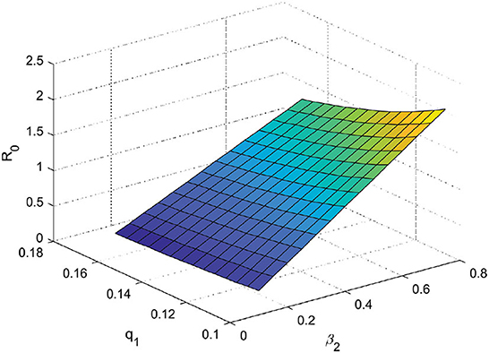
Figure 6. Effect parameters of R₀ (β₂ × q₁ ∈ [0.1 : 0.79664] × [0.1 : 0.16574]).

5. Optimal control problem

5.1. Comorbidity COVID-19 model with optimal control

The control variable given to the COVID-19 model consists of preventive measures through education (u₁) and individual treatment efforts for infected (u₂). So the model with control is given as follows:

$\begin{array}{l}\frac{dS}{dt}=\pi -(1-u_1)\frac{({\beta }_{1}SI+{\beta }_{2}SC)}{N}-q_{1}S-\mu S,\\ \frac{dE}{dt}=(1-u_1)\frac{({\beta }_{1}SI+{\beta }_{2}SC)}{N}-\alpha E-\mu E,\\ \frac{dI}{dt}=\xi \alpha E-(h_1+u_2)I-r_{1}I-d_{1}I-\mu I,\\ \frac{dC}{dt}=(1-\xi )\alpha E-(h_2+u_2)C-r_{2}C-d_{2}C-\mu C,\\ \frac{dQ}{dt}=q_{1}S-\frac{{\rho }_1{\beta }_{1}QI}{N}-\frac{{\rho }_2{\beta }_{2}QC}{N}-r_{3}Q-\mu Q,\\ \frac{dH}{dt}=(\theta h_1+u_2)I+\frac{p{\rho }_1{\beta }_{1}QI}{N}\\ +\frac{q{\rho }_2{\beta }_{2}QC}{N}+(\delta h_2+u_2)C-r_{4}H-d_{3}H-\mu H,\\ \frac{dJ}{dt}=((1-\theta )h_1+u_2)I\\ +((1-\delta )h_2+u_2)C+\frac{(1-p){\rho }_1{\beta }_{1}QI}{N}\\ +\frac{(1-q){\rho }_2{\beta }_{2}QC}{N}-a_{7}J,\\ \frac{dR}{dt}=r_{1}I+r_{2}C+r_{3}Q+r_{4}H+r_{5}J-\mu R.& (15)\end{array}$

The function that minimizes the number of infected cases without comorbidity (I) and the number of infected cases with comorbidity (C) over a time interval [0, T] can be defined as

$\begin{array}{ll}J(u_1,u_2)={\displaystyle {\int }_0^T}\left(I(t)+C(t)+\frac{1}{2}(A_1{u}_1^2+A_2{u}_2^2)\right),& (16)\end{array}$

Where A₁ and A₂ are the relative cost associated with the controls u₁ and u₂, and T is the final time. The aim of the control is to minimize the cost function.

$\begin{array}{l}J(u_1^{*},u_2^{*})=\text{min }J(u_1,u_2),\end{array}$

Subject to the system (Equation 15), where 0 ≤ (u₁, u₂) ≤ 1 and t ∈ (0, T).

5.2. Optimal control analysis

The Hamilton function can be defined as follows:

$\begin{array}{l}{H}=I+C+\frac{1}{2}\left(A_1{u}_1^2+A_2{u}_2^2\right)\\ +{\lambda }_1\left(\pi -\left(1-u_1\right)\frac{\left({\beta }_{1}SI+{\beta }_{2}SC\right)}{N}-q_{1}S-\mu S\right)\\ +{\lambda }_2\left(\left(1-u_1\right)\frac{\left({\beta }_{1}SI+{\beta }_{2}SC\right)}{N}-\alpha E-\mu E\right)\\ +{\lambda }_3\left(\xi \alpha E-\left(h_1+u_2\right)I-r_{1}I-d_{1}I-\mu I\right)\\ +{\lambda }_4\left(\left(1-\xi \right)\alpha E-\left(h_2+u_2\right)C-r_{2}C-d_{2}C-\mu C\right)\\ +{\lambda }_5\left(q_{1}S-\frac{{\rho }_1{\beta }_{1}QI}{N}-\frac{{\rho }_2{\beta }_{2}QC}{N}-r_{3}Q-\mu Q\right)\\ +{\lambda }_6(\left(\theta h_1+u_2\right)I+\frac{p{\rho }_1{\beta }_{1}QI}{N}\\ +\frac{q{\rho }_2{\beta }_{2}QC}{N}+\left(\delta h_2+u_2\right)C-r_{4}H-d_{3}H-\mu H)\\ +{\lambda }_7(\left(\left(1-\theta \right)h_1+u_2\right)I+\left(\left(1-\delta \right)h_2+u_2\right)C\\ +\frac{\left(1-p\right){\rho }_1{\beta }_{1}QI}{N}+\frac{\left(1-q\right){\rho }_2{\beta }_{2}QC}{N}-a_{7}J)\\ +{\lambda }_8\left(r_{1}I+r_{2}C+r_{3}Q+r_{4}H+r_{5}J-\mu R\right).& (17)\end{array}$

Based on Pontryagin's principle, the Hamilton function will reach an optimal solution if it satisfies the state equation and the costate equation, and the condition is stationary. The equation state is obtained by deriving the Hamilton function (Equation 17) for each variable costate as Equation (15). Next, the equation costate is the negative value of the derivative of the Hamilton function (Equation 17) for each variable state as follows:

$\begin{array}{l}\frac{d{\lambda }_1}{dt}=-\frac{\partial H}{\partial S}=\left({\lambda }_1-{\lambda }_2\right)\\ \left(\frac{\left(1-u_1\right)\left({\beta }_{1}I+{\beta }_{2}C\right)}{N}+\frac{\left(1-u_1\right)\left({\beta }_{1}SI+{\beta }_{2}SC\right)}{N^2}\right)\\ +q_1\left({\lambda }_1-{\lambda }_5\right)+{\lambda }_1\mu \\ +\frac{{\rho }_1{\beta }_{1}QI}{N^2}\left(p{\lambda }_6+\left(1-p\right){\lambda }_7-{\lambda }_5\right)\\ +\frac{{\rho }_2{\beta }_{2}QC}{N^2}\left(q{\lambda }_6+\left(1-q\right){\lambda }_7-{\lambda }_5\right),\\ \frac{d{\lambda }_2}{dt}=-\frac{\partial H}{\partial E}=\left({\lambda }_2-{\lambda }_1\right)\frac{\left(1-u_1\right)\left(CS{\beta }_2+IS{\beta }_1\right)}{N^2}\\ +{\lambda }_2\alpha +{\lambda }_2\mu -{\lambda }_3\alpha \xi -{\lambda }_4\alpha \left(1-\xi \right)\\ +\frac{{\rho }_1{\beta }_{1}QI}{N^2}\left({\lambda }_{6}p+\left(1-p\right){\lambda }_7-{\lambda }_5\right)+\frac{{\rho }_2{\beta }_{2}QC}{N^2}\\ \left({\lambda }_{6}q+\left(1-q\right){\lambda }_7-{\lambda }_5\right),\\ \frac{d{\lambda }_3}{dt}=-\frac{\partial H}{\partial I}=\left({\lambda }_1-{\lambda }_2\right)\left(\frac{\left(1-u_1\right)S{\beta }_1}{N}-\frac{\left(1-u_1\right)S{\beta }_1}{N}\right)\\ +h_1\left({\lambda }_3-\theta {\lambda }_6-\left(1-\theta \right){\lambda }_7\right)\\ +u_2\left({\lambda }_3-{\lambda }_6-{\lambda }_7\right)+r_1\left({\lambda }_3-{\lambda }_8\right)-{\lambda }_3\left(-d_1-\mu \right)\\ +\frac{{\rho }_1{\beta }_{1}Q}{N}\left({\lambda }_5-{\lambda }_{6}p-{\lambda }_7\left(1-p\right)\right)-1,\\ \frac{d{\lambda }_4}{dt}=-\frac{\partial H}{\partial C}\\ =\left({\lambda }_2-{\lambda }_1\right)\left(-\frac{\left(1-u_1\right)S{\beta }_2}{N}+\frac{\left(1-u_1\right)\left(CS{\beta }_2+IS{\beta }_1\right)}{N^2}\right)\\ +h_2\left({\lambda }_4-{\lambda }_6\delta -{\lambda }_7\left(1-\delta \right)\right)\\ +r_2\left({\lambda }_4-{\lambda }_8\right)+u_2\left({\lambda }_4-{\lambda }_6-{\lambda }_7\right)-{\lambda }_4\left(-d_2-\mu \right)\\ +\frac{{\rho }_1{\beta }_{1}QI}{N^2}\left(-{\lambda }_5+{\lambda }_{6}p+{\lambda }_7\left(1-p\right)\right)\\ +\left(\frac{{\rho }_2{\beta }_{2}Q}{N}-\frac{{\rho }_2{\beta }_{2}QC}{N^2}\right)\left({\lambda }_5-{\lambda }_{6}q-{\lambda }_7\left(1-q\right)\right)-1,\\ \frac{d{\lambda }_5}{dt}=-\frac{\partial H}{\partial Q}=\left({\lambda }_2-{\lambda }_1\right)\left(\frac{\left(1-u_1\right)\left(CS{\beta }_2+IS{\beta }_1\right)}{N^2}\right)\\ +r_3\left({\lambda }_5-{\lambda }_8\right)\\ +\left(\frac{{\rho }_1{\beta }_{1}I}{N}-\frac{{\rho }_1{\beta }_{1}QI}{N^2}\right)\left({\lambda }_5-p{\lambda }_6-\left(1-p\right){\lambda }_7\right)\\ +\left(\frac{{\rho }_2{\beta }_{2}C}{N}-\frac{{\rho }_2{\beta }_{2}QC}{N^2}\right)\left({\lambda }_5-{\lambda }_{6}q-{\lambda }_7\left(1-q\right)\right)+{\lambda }_5\mu ,\\ \frac{d{\lambda }_6}{dt}=-\frac{\partial H}{\partial H}=\left({\lambda }_2-{\lambda }_1\right)\left(\frac{\left(1-u_1\right)\left(CS{\beta }_2+IS{\beta }_1\right)}{N^2}\right)\\ +r_4\left({\lambda }_6-{\lambda }_8\right)+\frac{{\rho }_1{\beta }_{1}QI}{N^2}\left(-{\lambda }_5+{\lambda }_{6}p+{\lambda }_7\left(1-p\right)\right)\\ +\frac{{\rho }_2{\beta }_{2}QC}{N^2}\left(-{\lambda }_5+{\lambda }_{6}q+{\lambda }_7\left(1-q\right)\right),\\ \frac{d{\lambda }_7}{dt}=-\frac{\partial H}{\partial J}=\left({\lambda }_2-{\lambda }_1\right)\left(\frac{\left(1-u_1\right)\left(CS{\beta }_2+IS{\beta }_1\right)}{N^2}\right)\\ +r_5\left({\lambda }_7-{\lambda }_8\right)+\frac{{\rho }_1{\beta }_{1}QI}{N^2}\left(-{\lambda }_5+{\lambda }_{6}p+{\lambda }_7\left(1-p\right)\right)\\ +\frac{{\rho }_2{\beta }_{2}QC}{N^2}\left(-{\lambda }_5+{\lambda }_{6}q+{\lambda }_7\left(1-q\right)\right)+{\lambda }_7\left(d_4+\mu \right),\\ \frac{d{\lambda }_8}{dt}=-\frac{\partial H}{\partial R}=\left({\lambda }_2-{\lambda }_1\right)\left(\frac{\left(1-u_1\right)\left(CS{\beta }_2+IS{\beta }_1\right)}{N^2}\right)\\ +\frac{{\rho }_1{\beta }_{1}QI}{N^2}\left(-{\lambda }_5+{\lambda }_{6}p+{\lambda }_7\left(1-p\right)\right)\\ +\frac{{\rho }_2{\beta }_{2}QC}{N^2}\left(-{\lambda }_5+{\lambda }_{6}q+{\lambda }_7\left(1-q\right)\right)+{\lambda }_8\mu .& (18)\end{array}$

With transverse condition λ₁(T) = λ₂(T) = λ₃(T) = λ₄(T) = λ₅(T) = λ₆(T) = λ₇(T) = λ₈(T) = 0.

The stationary condition for the optimal control problem (16) is obtained by deriving the Hamilton function (17) on the control variables u₁ and u₂ $\left(\frac{\partial {H}}{\partial u_1}=0,\frac{\partial {H}}{\partial u_2}=0\right),$ successively obtained

$\begin{array}{l}{u}_1=\frac{({\beta }_{1}SI+{\beta }_{2}SC)({\lambda }_2-{\lambda }_1)}{N{A}_1}\text{ and}\\ u_2=\frac{I({\lambda }_3-{\lambda }_6-{\lambda }_7)+C({\lambda }_4-{\lambda }_6-{\lambda }_7)}{A_2}.\end{array}$

The control variables in the COVID-19 model with preventive measures through education and treatment efforts for infected individuals are defined as 0 ≤ u₁ ≤ 1 and 0 ≤ u₂ ≤ 1. So, the optimal control $u_1^{*}$ and $u_2^{*}$ can be expressed as

$\begin{array}{l}{u}_1^{*}=\text{maks}\left\{0,\text{min}\left(\frac{({\beta }_1{S}^{*}{I}^{*}+{\beta }_2{S}^{*}{C}^{*})({\lambda }_2-{\lambda }_1)}{N{A}_1},1\right)\right\}\text{and}\\ u_2^{*}=\text{maks}\left\{0,\text{min}\left(\frac{I^{*}({\lambda }_3-{\lambda }_6-{\lambda }_7)+C^{*}({\lambda }_4-{\lambda }_6-{\lambda }_7)}{A_2},1\right)\right\}.\end{array}$

The optimal system is obtained by substituting the optimal control variables $u_1^{*}$ and $u_2^{*}$ into the system of state (Equation 15) and costate (Equation 18) equations.

6. Simulation of the model with control

The method used in solving this optimal control problem is the forward–backward sweep method. In this numerical simulation, the parameter values used are presented in Table 1 according to the state of the COVID-19 case in Indonesia. Next, the initial values given are as follows S₀ = 270, 911, 990, E₀ = 1, 000, 000, I₀ = 412, 784, C₀ = 500, 000, Q₀ = 100, 000, H₀ = 56, 899, J₀ = 200, 000, and R₀ = 341, 942, with simulation intervals t ∈ [0, 100]. The results of the optimal numerical control simulation are presented as follows:

6.1. Using the control strategy u₁ ≠ 0 and u₂ = 0

Figure 7 shows the control strategy u₁ ≠ 0 and u₂ = 0. This is the result of education that makes all individuals always be careful, such as interacting outside the home. Implementing this strategy on subpopulations exposed, infected with comorbidity, infected without comorbidity, and isolation is significantly reduced. Implementing the control strategy u₁ ≠ 0 and u₂ = 0 can also increase the subpopulation of quarantine. Furthermore, the control strategy profiles u₁ ≠ 0 and u₂ = 0 to reduce the number of COVID-19 cases during t = 100 are presented in Figure 8.

FIGURE 7

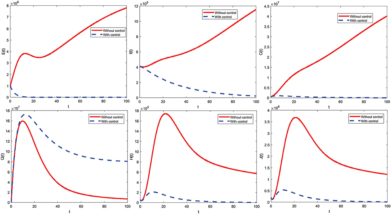
Figure 7. The optimal control simulation results with u₁ ≠ 0.

FIGURE 8

Figure 8. The optimal control profile with u₁ ≠ 0.

The control strategy u₁ ≠ 0 and u₂ = 0 is given by one (maximum) from the beginning of the period to t = 99.9 and decreases significantly to zero at the end of the period. Control is terminated at the period's end, meaning no more control is given.

6.2. Using the control strategy u₁ = 0 and u₂ ≠ 0

Figure 9 shows the control strategy u₁ = 0 and u₂ ≠ 0. This strategy can reduce the subpopulation infected with comorbid and without comorbid because there is an increase in the care of infected individuals. Implementing this strategy on subpopulations exposed, infected with comorbidity, infected without comorbidity, and isolation is significantly reduced. Implementing the control strategies u₁ = 0 and u₂ ≠ 0 can also increase the subpopulation of quarantine. Furthermore, the profiles of u₁ = 0 and u₂ ≠ 0 control strategies to reduce the number of COVID-19 cases for t = 100 are presented in Figure 10.

FIGURE 9

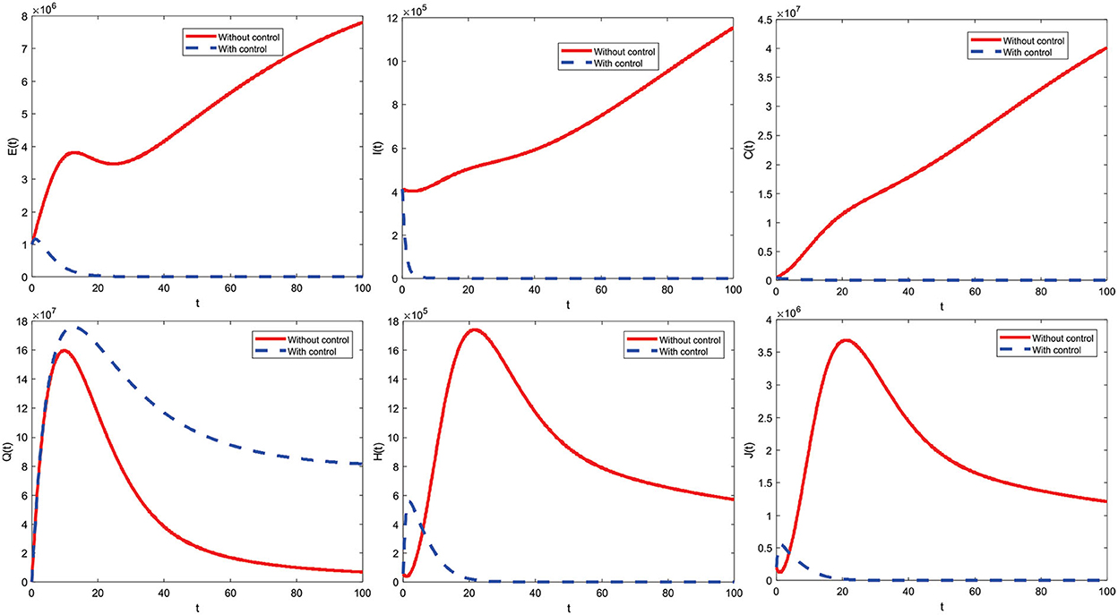
Figure 9. The optimal control simulation results with u₂ ≠ 0.

FIGURE 10

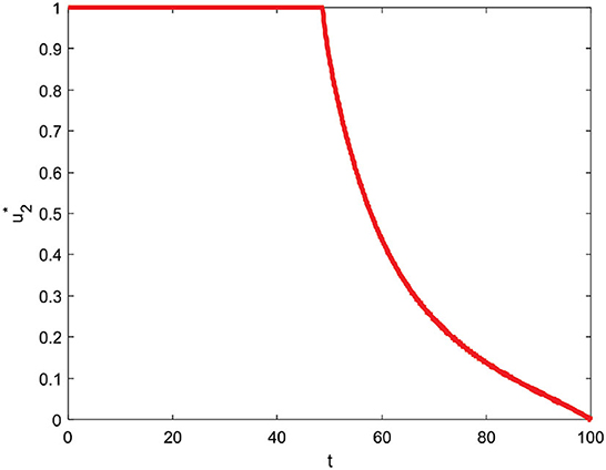
Figure 10. Optimal control profile with u₂ ≠ 0.

The control strategy u₁ = 0 and u₂ ≠ 0 is given by one (maximum) from the beginning to t = 48.6 and decreases slowly until t = 100 reaches zero which means control is stopped at the end of the period.

6.3. Using the control strategy u₁ ≠ 0 and u₂ ≠ 0

Figure 11 indicates a combined control strategy. This results from education that makes all individuals always be careful (such as interacting outside the home) and increased care for infected individuals. Combined control strategies can control or reduce deployment significantly. Furthermore, the combined control strategy profile to reduce the number of COVID-19 cases during t = 100 is presented in Figure 12.

FIGURE 11

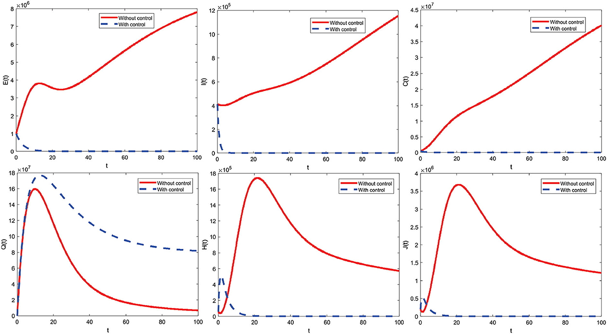
Figure 11. Combined optimal control simulation results.

FIGURE 12

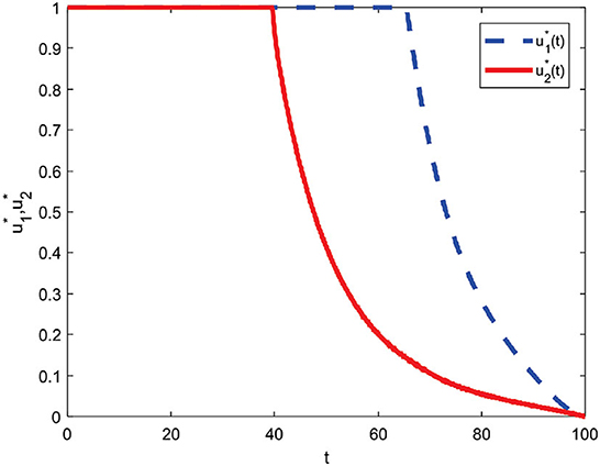
Figure 12. Combined control profile.

The combined control strategy consists of two concurrent administrations of control. The control u₁ is given by one (maximum) up to t = 65.4 and decreases significantly until the end of the period reaches zero. Then, control u₂ is assigned one (maximum) until t = 39.5 and then decreases until t = 100 slowly reaches zero. Both controls are terminated at the end of the period, which means they are no longer given control of u₁ and u₂.

6.4. Comparison of total infections using all strategic control scenarios

The varying initial values of the exposed subpopulations are given. Total infected subpopulations for different initial conditions from exposed subpopulations are E(0) = 200000, E(0) = 1000000, E(0) = 10000000, and E(0) = 100000000 successively from left to right using the three control strategies shown in Figure 13.

FIGURE 13

Figure 13. (A–D) Total subpopulation infected using various strategies.

From Figure 13, it can be seen that the number of infected subpopulations was reduced by applying the third strategy compared to other strategies. Based on strategies 1–3, it can be concluded that strategy 3 is the best strategy to minimize the number of people infected with COVID-19 in the community.

7. Cost evaluation

The cost evaluation aims to determine the most minimal cost-effectiveness strategy of COVID-19 spread control measures. Cost evaluation in this study uses average cost-effectiveness ratio (ACER) and incremental cost-effectiveness ratio (ICER). According to the approach to cost-effectiveness analysis, ACER is defined mathematically as follows:

$\begin{array}{l}ACER=\frac{\text{Objective function }(J)}{\text{Total number of infections averted}}.\end{array}$

The strategy with the smallest ACER value is the most cost-effective and is obtained in Table 4 as follows:

The incremental cost-effectiveness ratio, which compares two intervention options vying for the same scarce resources, typically tracks costs and health benefits changes. ICER is defined as follows when considering strategies p and q as two competing control intervention techniques:

$\begin{array}{l}ICER=\frac{\text{Change in total costs in strategies p and q}}{\text{Change in control benefits in strategies p and q}}.\end{array}$

Next, ICER was calculated to determine the most cost-effective strategy out of all the control strategies. First, the competition for strategies 1 and 2 is calculated as follows:

$\begin{array}{l}ICER(1)=\frac{49,247,000,000-0}{53,846,000,000-0}=0.9146,\\ ICER(2)=\frac{2,991,000,000-49,247,000,000}{53,893,000,000}\\ -53,846,000,000=-\frac{46,256,000,000}{47,000,000}=-984.1702,\end{array}$

The ICER results in strategy 1 were greater than in strategy 2, so educational controls alone were more expensive and ineffective than medical care enhancement controls. Therefore, strategy 1 is removed from the possible control strategies. Next, the ICER for strategies 2 and 3 is recalculated as follows:

$\begin{array}{l}ICER(2)=\frac{2,991,000,000-0}{53,893,000,000-0}=0.5130,\\ ICER(3)=\frac{1,794,700,000-2,991,000,000}{53,894,000,000-53,893,000,000}\\ =-\frac{1,196,300,000}{1,000,000}=-1,196.3.\end{array}$

Strategy 2 has a higher ICER value than strategy 3. So, strategy 3 (combined control) is the best control strategy of all options because of its cost-effectiveness and prevention of the spread of infectious diseases.

TABLE 4

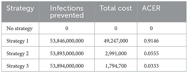
Table 4. Total infections prevented, total costs, and ACER for strategies 1, 2, and 3.

8. Conclusion

In this study, we have proposed a mathematical model of COVID-19 with comorbidities and added control of community education and improvement of medical care. The proposed model has been calibrated using cumulative confirmed infection cases in Indonesia. The basic reproduction number has been calculated by the next-generation matrix method. The model has an asymptotically stable disease-free equilibrium, provided that the basic reproduction number is <1. Furthermore, the model has an asymptotically stable endemic equilibrium, provided that the basic reproduction number is more than one. Individuals with comorbidity have a greater risk of infection, so there is a need for more supervision and preventive measures such as wearing masks, maintaining distance, and proper sanitation. Public education can be through social media, TV, radio, print media, and others to control the COVID-19 pandemic in Indonesia. Based on the model analysis, it is found that the COVID-19 pandemic can be controlled and eradicated if the value of R₀ < 1 by providing public education control and improving medical care. The sensitivity analysis results show that the most influential parameters are quarantine and contact with infected individuals, so educating the public to reduce disease transmission is important. After public education was given, the community became aware of the COVID-19 outbreak and began to reduce contact with other people. Likewise, the Indonesian government imposed large-scale social restrictions (PSBB) and enforced restrictions on community activities (PPKM) with four levels aiming to reduce infection and reduce social contact, educational institutions conducted online classes, webinars, etc. In addition to public education, increased medical care also need to be given to individuals who are already infected so that they recover quickly and that the epidemic is resolved soon. Furthermore, from the numerical results and cost-effectiveness analysis on the optimal control problem, it is found that applying a combination of controls can give the best results compared to a single control. This study can be extended in various ways, including considering the stochastic, time delay, and fractional derivative versions of this model. In addition, providing control variations (such as the presence of vaccination) combines the dynamics of two COVID-19 strains with another comorbidity and considers the COVID-19 vaccination model.

Data availability statement

The raw data supporting the conclusions of this article will be made available by the authors, without undue reservation.

Author contributions

MAR and F: conceptualization. MAR: methodology, software, writing—original draft preparation, and visualization. MAR, F, CA, and CWC: validation, investigation, and data curation. F, CA, and CWC: formal analysis. MAR, F, and CA: writing—review and editing. F and CA: supervision. All authors have read and agreed to the published version of the manuscript.

Conflict of interest

The authors declare that the research was conducted in the absence of any commercial or financial relationships that could be construed as a potential conflict of interest.

Publisher's note

All claims expressed in this article are solely those of the authors and do not necessarily represent those of their affiliated organizations, or those of the publisher, the editors and the reviewers. Any product that may be evaluated in this article, or claim that may be made by its manufacturer, is not guaranteed or endorsed by the publisher.

References

1. WHO. Novel Coronavirus. (2020). Available online at: https://www.who.int/indonesia/news/novel-coronavirus

Google Scholar

2. Wu Z, McGoogan JM. Characteristics of and important lessons from the coronavirus disease 2019 (COVID-19) outbreak in China: summary of a report of 72 314 cases from the Chinese center for disease control and prevention. JAMA. (2020) 323:1239–42. doi: 10.1001/jama.2020.2648

PubMed Abstract | CrossRef Full Text | Google Scholar

3. Kemkes. Pertanyaan dan Jawaban Terkait COVID-19 Kementerian Kesehatan. (2020). Available online at: https://www.kemkes.go.id/article/view/20030400008/FAQ-Coronavirus.html

4. WHO. Novel Coronavirus (COVID-19). (2021). Available online at: https://www.moh.gov.sa/en/HealthAwareness/EducationalContent/Corona/Pages/corona.aspx

Google Scholar

5. WHO. Novel Coronavirus (2019-nCoV): Situation Report 1. (2020). Available online at: https://apps.who.int/iris/handle/10665/330760

Google Scholar

6. Wu YC, Chen CS, Chan YJ. The outbreak of COVID-19: an overview. J Chin Med Assoc. (2020) 83:217–20. doi: 10.1097/JCMA.0000000000000270

PubMed Abstract | CrossRef Full Text | Google Scholar

7. Guan W, Liang W, Zhao Y, Liang H, Chen Z, Li Y, et al. Comorbidityity and its impact on 1590 patients with COVID-19 in China: a nationwide analysis. Eur Respir J. (2020) 55:2000547. doi: 10.1183/13993003.00547-2020

PubMed Abstract | CrossRef Full Text | Google Scholar

8. Yang J, Zheng Y, Gou X, Pu K, Chen Z, Guo Q. International journal of infectious diseases prevalence of comorbidities and its effects in patients infected with SARS-CoV-2: a systematic review and meta-analysis. Int J Infect Dis. (2020) 94:91–5. doi: 10.1016/j.ijid.2020.03.017

PubMed Abstract | CrossRef Full Text | Google Scholar

9. Satgas. Peta Sebaran COVID-19. (2021). Available online at: https://covid19.go.id/peta-sebaran

10. Adisasmito W, Suwandono A, Trihono, Gani A, Aisyah DN, Solikha DA, et al. Studi komparasi pembelajaran penanganan COVID-19 Indonesia-Korea Selatan. In: Direktorat Kesehatan dan Gizi Masyarakat Kementerian PPN/BAPPENAS. (2021). Available online at: https://infeksiemerging.kemkes.go.id/document/download/3ax61Bxrn5

11. Worldometers. Report Coronavirus Cases (2021). Available online at: https://www.worldometers.info/coronavirus/

12. Lemon SM, Hamburg MA, Frederick P, Choffnes ER, Mack A. Ethical and Legal Considerations in Mitigating Pandemic Disease: Workshop Summary. Washington, DC: National Academic Press (2007).

PubMed Abstract | Google Scholar

13. WHO. COVID-19 Strategy Update. (2020). Available online at: https://www.who.int/publications/m/item/covid-19-strategy-update

Google Scholar

14. WHO. Pertimbangan-Pertimbangan Untuk Karantina Individu Dalam Konteks Penanggulangan Penyakit Coronavirus (COVID-19). (2020). Available online at: https://www.who.int/docs/default-source/searo/indonesia/covid19/who-2019-covid19-ihr-quarantine-2020-indonesian.pdf?sfvrsn=31d7cbd8_2

15. Tang B, Wang X, Li Q, Bragazzi NL, Tang S, Xiao Y, et al. Estimation of the transmission risk of the 2019-nCoV and its implication for public health interventions. J Clin Med. (2020) 9:462. doi: 10.3390/jcm9020462

PubMed Abstract | CrossRef Full Text | Google Scholar

16. Müller J, Kuttler C. Methods and Models in Mathematical Biology. Berlin; Heidelberg: Springer-Verlag (2015).

Google Scholar

17. Murray JD. Mathematical Biology I: An Introduction. Berlin; Heidelberg: Springer-Verlag (2002).

Google Scholar

18. Feng Z. Final and peak epidemic sizes for SEIR models with quarantine and isolation. Math Biosci Eng. (2007). 4:675–86. doi: 10.3934/mbe.2007.4.675

PubMed Abstract | CrossRef Full Text | Google Scholar

19. Tahir M, Shah SIA, Zaman G, Khan T. Stability behaviour of mathematical model MERS corona virus spread in population. Filomat. (2019) 33:3947–60. doi: 10.2298/FIL1912947T

CrossRef Full Text | Google Scholar

20. Usaini S, Hassan AS, Garba SM, Lubuma JMS. Modeling the transmission dynamics of the middle east respiratory syndrome coronavirus (MERS-CoV) with latent immigrants. J Interdisc Math. (2019) 22:903–30. doi: 10.1080/09720502.2019.1692429

CrossRef Full Text | Google Scholar

21. Soewono E. On the analysis of COVID-19 transmission in wuhan, diamond princess and jakarta-cluster. Commun Biomath Sci. (2020) 3:9–18. doi: 10.5614/cbms.2020.3.1.2

CrossRef Full Text | Google Scholar

22. Das P, Upadhyay RK, Misra AK, Rihan FA, Das P, Ghosh D. Mathematical model of COVID-19 with comorbidity and controlling using non-pharmaceutical interventions and vaccination. Nonlinear Dyn. (2021) 106:1213–27. doi: 10.1007/s11071-021-06517-w

PubMed Abstract | CrossRef Full Text | Google Scholar

23. Omame A, Sene N, Nometa I, Nwakanma CI, Nwafor EU, Iheonu NO, et al. Analysis of COVID-19 and comorbidity co-infection model with optimal control. Optimal Control Appl Methods. (2021) 42:1568–90. doi: 10.1002/oca.2748

PubMed Abstract | CrossRef Full Text | Google Scholar

24. Jia J, Ding J, Liu S, Liao G, Li J, Duan B, et al. Modeling the control of COVID-19: impact of policy interventions and meteorological factors. Electron J Diff Equ. (2020) 2020:23.

Google Scholar

25. Prathumwan D, Trachoo K, Chaiya I. Mathematical modeling for prediction dynamics of the coronavirus disease 2019 (COVID-19) pandemic, quarantine control measures. Symmetry. (2020) 12:1404. doi: 10.3390/sym12091404

CrossRef Full Text | Google Scholar

26. Deressa CT, Duressa GF. Modeling and optimal control analysis of transmission dynamics of COVID-19: The case of Ethiopia. Alexandria Eng J. (2020) 60:719–32. doi: 10.1016/j.aej.2020.10.004

CrossRef Full Text | Google Scholar

27. Olaniyi S, Obabiyi OS, Okosun KO, Oladipo AT, Adewale SO. Mathematical modelling and optimal cost-effective control of COVID-19 transmission dynamics. Eur Phys J Plus. (2020) 135:938. doi: 10.1140/epjp/s13360-020-00954-z

PubMed Abstract | CrossRef Full Text | Google Scholar

28. Aldila D, Khoshnaw SHA, Safitri E, Rais YA, Bakry ARQ, Samiadji BM, et al. A mathematical study on the spread of COVID-19 considering social distancing and rapid assessment: the case of Jakarta, Indonesia. Chaos Solit Fractals. (2020) 139:110042. doi: 10.1016/j.chaos.2020.110042

PubMed Abstract | CrossRef Full Text | Google Scholar

29. Aldila D, Ndii MZ, Samiadji BM. Optimal control on COVID-19 eradication program in Indonesia under the effect of community awareness. Math Biosci Eng. (2020) 17:6355–89. doi: 10.3934/mbe.2020335

PubMed Abstract | CrossRef Full Text | Google Scholar

30. Ali M, Shah STH, Imran M, Khan A. The role of asymptomatic class, quarantine and isolation in the transmission of COVID-19. J Biol Dyn. (2020) 14:389–408. doi: 10.1080/17513758.2020.1773000

PubMed Abstract | CrossRef Full Text | Google Scholar

31. Rois MA, Tafrikan M, Norasia Y, Anggriani I, Ghani M. SEIHR model on spread of COVID-19 and its simulation. Telematika. (2022) 15.

Google Scholar

32. Annas S, Pratama MI, Rifandi M, Sanusi W, Side S. Stability analysis and numerical simulation of SEIR model for pandemic COVID-19 spread in Indonesia. Chaos Solit Fractals. (2020) 139:110072. doi: 10.1016/j.chaos.2020.110072

PubMed Abstract | CrossRef Full Text | Google Scholar

33. Baba IA, Nasidi BA, Baleanu D. Optimal control model for the transmission of novel COVID-19. Comput Mater Continua. (2021) 66:3089–106. doi: 10.32604/cmc.2021.012301

CrossRef Full Text | Google Scholar

34. Li XP, Darassi MH, Khan MA, Chukwu CW, Alshahrani MY, Shahrani MA, et al. Assessing the potential impact of COVID-19 Omicron variant: insight through a fractional piecewise model. Results Phys. (2022) 38:105652. doi: 10.1016/j.rinp.2022.105652

PubMed Abstract | CrossRef Full Text | Google Scholar

35. Bajiya VP, Bugalia S, Tripathi JP. Mathematical modeling of COVID-19: impact of non-pharmaceutical interventions in india mathematical modeling of COVID-19: impact of non-pharmaceutical interventions in India. Chaos. (2020) 30:113143. doi: 10.1063/5.0021353

PubMed Abstract | CrossRef Full Text | Google Scholar

36. Das P, Nadim SS, Das S, Das P. Dynamics of COVID-19 transmission with comorbidity: a data driven modelling based approach. Nonlinear Dyn. (2021) 106:1197–211. doi: 10.1007/s11071-021-06324-3

PubMed Abstract | CrossRef Full Text | Google Scholar

37. Diagne ML, Rwezaura H, Tchoumi SY, Tchuenche JM. Mathematical model of COVID-19 with vaccination and treatment. Comput Math Methods Med. (2021) 2021:1250129. doi: 10.1155/2021/1250129

PubMed Abstract | CrossRef Full Text | Google Scholar

38. Ghostine R, Gharamti M, Hassrouny S, Hoteit I. An extended SEIR model with vaccination for forecasting the COVID-19 pandemic in Saudi Arabia using an ensemble Kalman filter. Mathematics. (2021) 9:636. doi: 10.3390/math9060636

CrossRef Full Text | Google Scholar

39. Kouidere A, Khajji B, Bhih AE, Balatif O, Rachik MA. Mathematical modeling with optimal control strategy of transmission of COVID-19 pandemic virus. Commun Math Biol Neurosci. (2020) 2020:24. doi: 10.28919/cmbn/4599

CrossRef Full Text | Google Scholar

40. Madubueze CE, Onwubuya IO, Dachollom S. Controlling the spread of COVID-19: optimal control analysis. Comput Math Methods Med. (2020) 2020:6862516. doi: 10.1101/2020.06.08.20125393

PubMed Abstract | CrossRef Full Text | Google Scholar

41. Naveed M, Baleanu D, Rafiq M, Raza A, Soori A, Hasan, et al. Dynamical behavior and sensitivity analysis of a delayed coronavirus epidemic model. Comput Mater Continua. (2020) 65:225–41. doi: 10.32604/cmc.2020.011534

CrossRef Full Text | Google Scholar

42. Riyapan P, Shuaib SE, Intarasit A. A mathematical model of COVID-19 pandemic: a case study of Bangkok, Thailand. Comput Math Methods Med. (2021) 2021:6664483. doi: 10.1155/2021/6664483

PubMed Abstract | CrossRef Full Text | Google Scholar

43. Yang C, Wang J. A mathematical model for the novel coronavirus epidemic in Wuhan, China. Math Biosci Eng. (2020) 17:2708–24. doi: 10.3934/mbe.2020148

PubMed Abstract | CrossRef Full Text | Google Scholar

44. Youssef HM, Alghamdi NA, Ezzat MA, El-bary AA, Shawky AM. Study on the SEIQR model and applying the epidemiological rates of COVID-19 epidemic spread in Saudi Arabia. Infect Dis Model. (2021) 6:678–92. doi: 10.1016/j.idm.2021.04.005

PubMed Abstract | CrossRef Full Text | Google Scholar

45. Youssef HM, Alghamdi NA, Ezzat MA, El-Bary AA, Shawky AM. A new dynamical modeling SEIR with global analysis applied to the real data of spreading COVID-19 in Saudi Arabia. Math Biosci Eng. (2020) 17:7018–44. doi: 10.3934/mbe.2020362

PubMed Abstract | CrossRef Full Text | Google Scholar

46. Rois MA, Trisilowati T, Habibah U. Dynamic analysis of COVID-19 model with quarantine and isolation. JTAM. (2021) 5:418–33.

Google Scholar

47. Rois MA, Trisilowati, Habibah U. Optimal control of mathematical model for COVID-19 with quarantine and isolation. Int J Eng Trends Technol. (2021) 69:154–60. doi: 10.14445/22315381/IJETT-V69I6P223

PubMed Abstract | CrossRef Full Text | Google Scholar

48. Musa SS, Qureshi S, Zhao S, Yusuf A, Mustapha UT, He D. Mathematical modeling of COVID-19 epidemic with effect of awareness programs. Infect Dis Model. (2021) 6:448–60. doi: 10.1016/j.idm.2021.01.012

PubMed Abstract | CrossRef Full Text | Google Scholar

49. Chukwu CW, Fatmawati. Modelling fractional-order dynamics of COVID-19 with environmental transmission and vaccination: a case study of Indonesia. AIMS Math. (2022) 7:4416–38. doi: 10.3934/math.2022246

CrossRef Full Text

50. Zeb A, Alzahrani E, Erturk VS, Zaman G. Mathematical Model for coronavirus disease 2019 (COVID-19) containing isolation class. BioMed Res Int. (2020) 2020:3452402. doi: 10.1155/2020/3452402

PubMed Abstract | CrossRef Full Text | Google Scholar

51. Bonyah E, Juga M, Fatmawati. Fractional dynamics of coronavirus with comorbidity via Caputo-Fabrizio derivative. Commun Math Biol Neurosci. (2022) 2022:12. doi: 10.28919/cmbn/6964

CrossRef Full Text | Google Scholar

52. Fatmawati, Yuliani E, Alfiniyah C, Juga ML, Chukwu CW. On the modeling of COVID-19 transmission dynamics with two strains: insight through caputo fractional derivative. Fractal Fract. (2022) 6:346. doi: 10.3390/fractalfract6070346

CrossRef Full Text | Google Scholar

53. Majumder M, Tiwari PK, Pal S. Impact of saturated treatments on HIV-TB dual epidemic as a consequence of COVID-19: optimal control with awareness and treatment. Nonlinear Dyn. (2022) 109:143–76. doi: 10.1007/s11071-022-07395-6

PubMed Abstract | CrossRef Full Text | Google Scholar

54. Rai RK, Khajanchi S, Tiwari PK, Venturino E, Misra AK. Impact of social media advertisements on the transmission dynamics of COVID-19 pandemic in India. J Appl Math Comput. (2022) 68:19–44. doi: 10.1007/s12190-021-01507-y

PubMed Abstract | CrossRef Full Text | Google Scholar

55. Brauer F, Castillo-Chavez C. Mathematical Models in Population Biology and Epidemiology. New York, NY: Springer-Verlag New York (2012).

Google Scholar

56. Driessche PVD, Watmough J. Reproduction numbers and sub-threshold endemic equilibria for compartmental models of disease transmission. Math Biosci. (2002) 180:29–48. doi: 10.1016/S0025-5564(02)00108-6

PubMed Abstract | CrossRef Full Text | Google Scholar

57. Alligood KT, Sauer TD, Yorke JA. CHAOS: an Introduction to dynamical systems. In: Introduction To Computational Modeling Using C and Open-Source Tools. New York, NY; Berlin; Heidelberg: Springer-Verlag (2000).

Google Scholar

58. Chitnis N, Hyman JM, Cushing JM. Determining important parameters in the spread of malaria through the sensitivity analysis of a mathematical model. Bull Math Biol. (2008) 70:1272. doi: 10.1007/s11538-008-9299-0

PubMed Abstract | CrossRef Full Text | Google Scholar

59. Rois MA, Trisilowati T, Habibah U. Local sensitivity analysis of COVID-19 epidemic with quarantine and isolation using normalized index. Telematika. (2021) 14:13–24. doi: 10.35671/telematika.v14i1.1191

CrossRef Full Text | Google Scholar