 Alexei Chekhlov
 Ilya Staroselsky
 Hudong Chen
95% of researchers rate our articles as excellent or good
Learn more about the work of our research integrity team to safeguard the quality of each article we publish.
Find out more
ORIGINAL RESEARCH article
Front. Appl. Math. Stat. , 11 January 2023
Sec. Mathematical Physics
Volume 8 - 2022 | https://doi.org/10.3389/fams.2022.1066522
Numerical simulation results of basic exactly solvable fluid flows using the previously proposed by H. Chen Lattice Boltzmann Method (LBM) formulated on a general curvilinear coordinate system are presented. As was noted in the theoretical work of H. Chen, such curvilinear Lattice Boltzmann Method preserves a fundamental one-to-one exact advection feature in producing minimal numerical diffusion, as the Cartesian lattice Boltzmann model. As we numerically show, the new model converges to exact solutions of basic fluid flows with the increase of grid resolution in the presence of both natural curvilinear geometry and/or grid non-uniform contraction, both for near equilibrium and non-equilibrium LBM parameter choices.
Lattice Boltzmann Method (LBM) is currently one of the most accurate and widely used methods of simulation and analysis of continuum media. In many physics and engineering applications, LBM almost completely displaced and/or replaced its direct finite-difference or finite-volume Navier-Stokes-based competitors. As it is well-known, currently used versions of variable grid LBM are based on the volumetric formulation of LBM [1] with the Cartesian formulation of lattice cells and space basis vectors and linear approximations of curved boundaries within a lattice cell and Variable Resolution (or VR)-regions [2, 3]. Their accuracy and consistency could be potentially improved if a true non-Cartesian formulation were available.
As was detailed in Chen [4], some attempts to achieve this goal were made in He et al. [5] and Barraza and Dieterding [6], albeit with a loss of a very important feature of the basic LBM—precision of the advection stage, and brought a significant amount of numerical dissipation. The adequate way to avoid this is to represent the process on a general coordinate system based on Riemann geometry [7] where particles move on a curved path in Euclidean space. Such a method should be producing a curvilinear inertial body force. Several such attempts were made in a series of papers [8–10].
Recently, a new approach [4] was proposed which for the first time has used a truly curvilinear tensor formulation of the Lattice Boltzmann Method. As noted in Chen [4], the following key differences to works [8–10] were proposed: the volumetric approach which exactly conserves the mass and momentum without a mass source, and also the curvilinear body force which adds momentum in the curvilinear space leads to the exact momentum conservation and reproduces the Navier-Stokes hydrodynamics to the viscous order.
The goal of this paper is to test and numerically validate this new method on several exactly solvable fluid flow cases in which non-equilateral lattices can be used and results can be compared with both analytical solutions and standard LBM. We have chosen the following four 2-dimensional test models: planar Couette and Poiseuille flows, with rectangular, but possibly non-equilateral, lattice cells, and circular Couette and Poiseuille flows, with strong effects of cells' natural curvilinearity.
We consider two LBM lattices: D2Q9 and D2Q21 with different degrees of moment isotropy. The D2Q9 has the moment isotropy up to the 4th order, whereas the D2Q21 has the moment isotropy up to the 6th order. In the first two of the considered—rectangular yet non-equilateral—cases, for both the D2Q9 and D2Q21 lattices we observe a very good convergence of the new numerical method [4] to the exact solution with resolution increase. In the second two cases characterized by the true naturally curvilinear lattice cells, we find that only the D2Q21 lattice leads to convergence to the exact solutions. Apparently, the D2Q9 4th-order moment isotropy is not sufficient for ensuring the accuracy of the new method, since the numerical method does converge to a solution that is however different from the exact one. Therefore, we conclude that the higher-order (6th or higher) moment isotropy of the lattice is required for the volumetric curvilinear LBM method [4].
We have studied both equilibrium cases with the LBM relaxation time τ = 1 and non-equilibrium cases with and confirmed that the method [4] works well for non-equilibrium cases as well.
In order to achieve our goals, we have generalized the LBM periodicity, no-slip, and moving wall boundary conditions to the fully curvilinear case. Additionally, as explained in more detail later, we have proposed an adjustment procedure using the "no flow" solution algorithm to adjust the effects of discrete finite-difference approximation for the generalized basis vectors definition in Chen [4].
In the next section, we review the theoretical approach formulated in Chen [4]. Then in Section 3, we present numerical results for the four basic flow cases mentioned above. In Section 4 we further discuss our findings as well some possible future work directions. In Appendix A, we discuss the properties of moments isotropy of the considered lattices D2Q9 and D2Q21. In Appendix B, we formulate the curvilinear boundary conditions. In Appendix C, we describe an example of a non-equidistant lattice used for this study.
In Chen [4], a volumetric lattice Boltzmann formulation on a general curvilinear mesh is constructed based on a one-to-one mapping between physical and computational spaces x = x(q) as follows. The coordinate values in the computational space {q} are defined exactly as in standard LBM, i.e., forming a 3D Cartesian lattice with the lattice spacing unity. The nearest neighbor of a site in the physical space x(q) along the ith (i = 1, 2, 3) coordinate direction in the positive or negative direction is a spatial point x±i = x(q±i), where q±i is a unique coordinate value for the neighboring site, so that and . This defines the distance vector from x(q) to one of its neighbors x(q±i):
which allows construction of the basis tangent vectors at x(q):
that have a number of standard differential geometry properties that can be found in Chen [4]. The metric tensor and the cell volume J at x(q) are thus defined as
and the co-tangent basis vectors gi(q) as well as the inverse metric tensor,
where ϵijk is a standard 3-dimensional Levy-Civita symbol.
With these definitions, we obtain the lattice Boltzmann velocity vectors on a general curvilinear mesh defined similar to the ones on a standard Cartesian lattice,
as well as a discrete analog of the Christoffel symbol,
Now, the evolution of particle distribution is defined in the computational space q similar to the standard isothermal lattice Boltzmann equation (LBE), Frisch et al. [11], Chen et al. [12, 13], Benzi et al. [14], and Qian et al. [15].
where Nα(q, t) is the number of particles belonging to the discrete direction cα in the cell q at time t. Here, Ωα(q, t) is the collision term that satisfies local mass and momentum conservation, and the particle density distribution function fα(q, t) is related to Nα(q, t) via
The fundamental fluid quantities such as density ρ(q, t) and velocity u(q, t) are given by the standard hydrodynamic moments,
Using the Equation (4), the velocity moment above can be rewritten as
and the velocity in the curvilinear coordinate system is given by:
Observe that the Equation (10) has the same form for the fluid velocity as that in the standard Cartesian lattice-based LBM. We will use a linearized LBM collision term [14, 16]:
where is the equilibrium distribution function and τ is the Bhatnagar-Gross-Krook (BGK) collision relaxation time [12, 13, 15, 17].
The extra term δNα(q, t) in the Equation (6) represents the change of particle distribution due to an effective inertial body force, which is a key feature of curvilinear geometry-based LBM, associated with the curvature and non-uniformity of a general curvilinear mesh. This inertial body force obviously vanishes in the standard LBM on a Cartesian lattice.
Define the advection process as an exact one-to-one hop from one site in the computational space to another as in the standard LBM:
where is the post-collide distribution at (q, t) that is equal to the right side of the Equation (6). In Chen [4] it was shown that the key intrinsic effect of curvilinear formulation, the net momentum change via advection from all the neighboring cells into cell q is given by:
and out of cell q to all its neighboring cells, is given by:
so that an “inertial force” χ(q, t) = [χI(q, t) + χo(q, t)]/2 that equals exactly to the amount needed for achieving the momentum conservation in the underlying Euclidean space is:
The full viscous Navier-Stokes equation is recovered when the momentum flux is defined as:
It is shown in Chen [4] that choosing:
satisfies the necessary moment constraints. Note also that due to the appearance of in the Equation (15), the overall collision process for determining defines an implicit relationship. Specifically, the Equation (17) defines the curvilinear correction δNα(q, t) through Fj(q, t) and the Equation (15) expresses Fj(q, t) using N′(q, t), which, again, depends on the same δNα(q, t). In this work, for the numerical implementation of the Equation (15) we split this implicit relationship into explicit relationships at two successive time steps: we use the from the previous time-step in the Equation (15). Iterative procedures to numerically implement this implicit relationship in the Equation (15) are also possible.
The physical velocity was defined in Chen [4] through the curvilinear body force F as follows:
The equilibrium distribution function that produces the Navier-Stokes equation in curvilinear coordinates in the hydrodynamic limit is Chen [4]:
We will also need the following simple mapping of fluid values ρ(q, t) and Ui(q, t) onto the original curvilinear mesh:
The four exactly solvable flow problems are presented below in order to validate the new approach [4]. As stated in Chen [4], in order to recover the correct isothermal low Ma Navier-Stokes hydrodynamics, a set of necessary moments isotropy and normalization conditions must be satisfied. This is why we present a detailed comparison between two lattices: D2Q9 and D2Q21. The details of isotropy and normalization conditions for these two lattices are presented in Appendix A. In all of the below cases, we use the boundary conditions, generalized by us for curvilinear LBM, presented in detail in Appendix B.
This well-known [18] simple exact solution describes a stationary flow of viscous incompressible fluid between two vertical planes: at x = 0 moving with a constant velocity , and a non-moving one at x = l:
Solution of the Equation (21) in lattice units for a non-equidistant lattice is:
Here xi is a spatially varying coordinate of the lattice node. In this study, a lattice that is linearly contracting toward the boundaries is used (see Appendix C), and is the average step in the x-direction. We studied other variable-size lattices and conclude that our main findings do not depend on the particular type of contraction, as long as some general stability conditions are satisfied.
Thus, defined plane channel problem does not possess a true curvilinearity but rather a deviation from the equidistant lattice which is due to cell contraction.
The LBM parameters for the equilibrium case with τ = 1 for the D2Q9 lattice are listed in Table 1A:
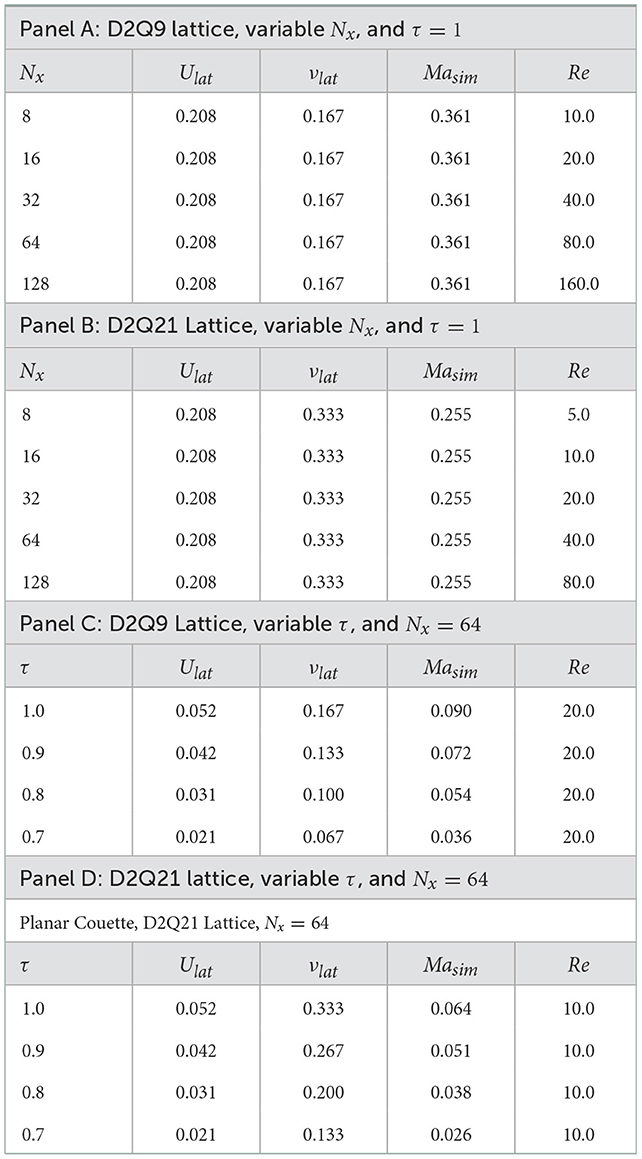
Table 1. Planar Couette LBM parameters.
As it is well expected, on the equidistant D2Q9 lattice (which corresponds to the trivial compression ratio CR = 0 in our notations), all quantities ρ(x), 1(x) and 2(x) for all resolutions Nx = 8, 16, 32, 64, 128 accurately reproduce the exact analytical solution (Equations 21, 22).
One simple way to introduce some curvilinear effects into an otherwise Cartesian geometry is to consider variable aspect ratio grid cells, for example as is done in the linear grid compression case described in Appendix C. An example of such geometry and grid is shown in Figure 1A.
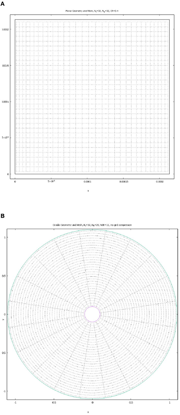
Figure 1. Examples of Geometries and Lattices Considered. (A) Cartesian geometry case with Nx = Ny = 32, and linear CR = 0.4 grid compression in x−direction. (B) Circular geometry case with Nr = 32, Nθ = 20, and NCR = 11.
The numerical results for the fields of ρ(x) and 2(x) for the D2Q9 lattice with the nontrivial compression ratio CR = 0.4, are presented in Figures 2A, B below:
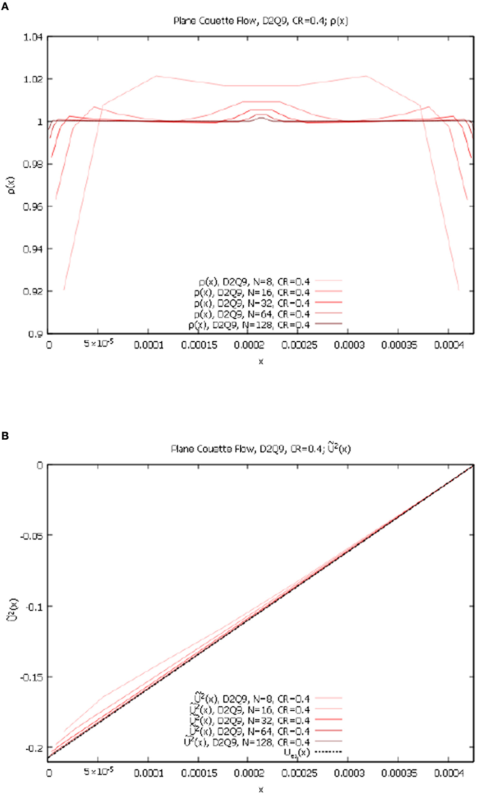
Figure 2. Planar Couette flow, contracting grid, variable Nx, D2Q9 lattice. (A) ρ(x) for Nx = 8, 16, 32, 64, 128 and CR = 0.4. (B) 2(x) for Nx = 8, 16, 32, 64, 128, and CR = 0.4.
1(x) in this case is negligibly small for all resolutions Nx = 8, 16, 32, 64, 128. As we can see, even on strongly non-equidistant lattice D2Q9 we also converge to the exact solution with higher resolutions.
The LBM parameters for the D2Q21 lattice and τ = 1 that we used are listed in the Table 1B above.
The boundary conditions developed for curvilinear LBM with D2Q21 are presented in Appendix B. In formulating the boundary conditions, we have assumed the symmetrically-continued geometry through the boundary. The stencil length for D2Q21 is three times larger than that for D2Q9, and therefore some approximation errors are expected to be larger near the moving boundary than those for D2Q9. It needs to be pointed out that this issue is related to the boundary conditions algorithm rather than to the intrinsic nature of the curvilinear LBM [4].
Similar to the D2Q9 case, our code applied to the trivial equilateral D2Q21 lattice (CR = 0) gives perfectly converging results for all ρ(x), 1(x), and 2(x), for all resolutions Nx = 8, 16, 32, 64, 128 that accurately reproduce the exact analytical solution (Equations 21, 22). Results for ρ(x) and 2(x) for D2Q21 and nontrivial rectangular lattice with CR = 0.4 are presented in Figures 3A, B below. Note that CR = 0.4 corresponds to and , and that according to our set-up of the linearly contracting lattice described in Appendix C, this value of CR corresponds to different values of lattice parameter a for each resolution.
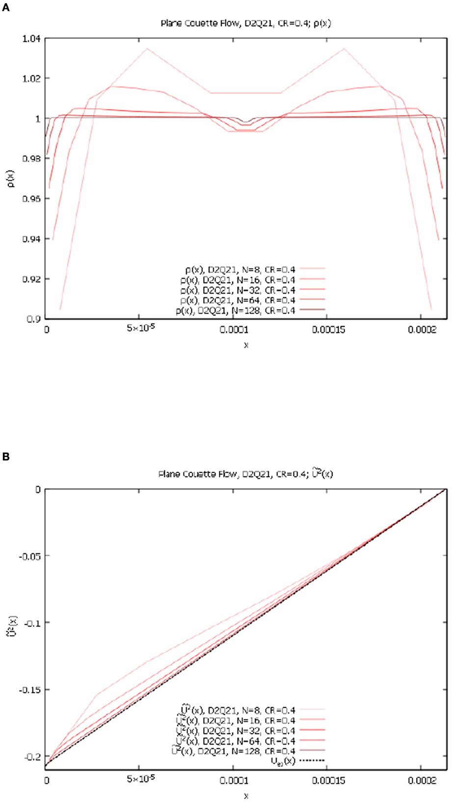
Figure 3. Planar Couette flow, contracting grid, variable Nx, D2Q21 lattice. (A) ρ(x) for Nx = 8, 16, 32, 64, 128 and CR = 0.4. (B) 2(x) for Nx = 8, 16, 32, 64, 128, and CR = 0.4.
As we can see, even on strongly non-equidistant lattice D2Q21 we also converge to the exact solution with higher resolutions.
Let us now present the results of numerical model solutions for a fixed resolution Nx = 64 but variable τ = {1.0, 0.9, 0.8, 0.7} for both lattices D2Q9 and D2Q21.
The corresponding LBM parameters for the D2Q9 lattice we used are listed in Table 1C above.
The agreement of numerical solution with the exact one with no lattice compression CR = 0 is of course very good for both lattices D2Q9 and D2Q21 for all τ = {1.0, 0.9, 0.8, 0.7}. In Figures 4A, B below we present the comparisons of numerical results with the exact solution for lattice D2Q9 with compression CR = 0.35 and τ = {1.0, 0.9, 0.8, 0.7}. We show variable τ cases on the same graphs, for the following quantities: , and .
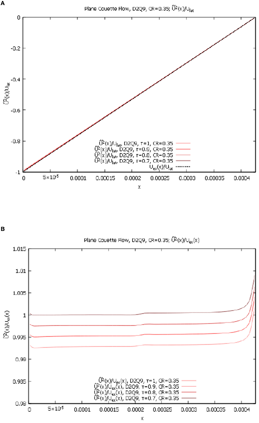
Figure 4. Planar Couette flow, contracting grid, variable τ for D2Q9 lattice. (A) for D2Q9, τ = 1.0, 0.9, 0.8, 0.7, and CR = 0.35. (B) for D2Q9, τ = 1.0, 0.9, 0.8, 0.7, and CR = 0.35.
The for D2Q9, τ = 1.0, 0.9, 0.8, 0.7, and CR = 0.35, are all equal to zero within double-precision accuracy and the for D2Q9, τ = 1.0, 0.9, 0.8, 0.7, and CR = 0.35 show very weak dependence on τ. We can see that for D2Q9 lattice and strong cell compression the new method [4] not only converges with the increase in resolution but also works well for various values of parameter τ.
The corresponding LBM parameters used for the D2Q21 lattice are listed in Table 1D above. Similar numerical results for D2Q21 lattice are presented in Figures 5A, B below.
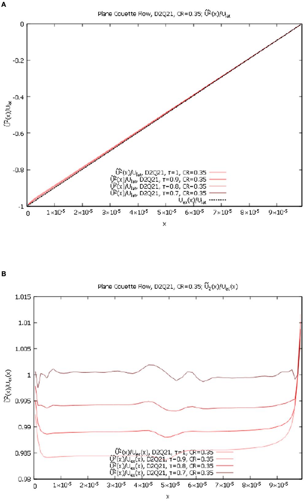
Figure 5. Planar Couette flow, contracting grid, variable τ for D2Q21 lattice. (A) for D2Q21, τ = 1.0, 0.9, 0.8, 0.7, and CR = 0.35. (B) for D2Q21, τ = 1.0, 0.9, 0.8, 0.7, and CR = 0.35.
As in the D2Q9 case, the for D2Q21, τ = 1.0, 0.9, 0.8, 0.7, and CR = 0.35, are approximately equal to zero and the for D2Q21, τ = 1.0, 0.9, 0.8, 0.7, and CR = 0.35 show very weak dependence on τ. Here we can also see that for D2Q21 lattice with strong cell compression the new method [4] not only converges with the increase in resolution but also works well for various values of parameter τ.
All the problems considered in the paper were solved numerically as non-stationary problems converging to a steady state from zero initial velocity state. The convergence to the steady state was judged by the conservation of total kinetic energy in the system in the first two plane geometry problems and by the conservation of both total kinetic energy and total angular momentum in the system in the second two curvilinear (circular) problems. In order to achieve that steady state in some cases over 150 times to traverse the characteristic length with the characteristic velocity were required. Total mass in the system was conserved at all intermediary times.
Also note the fact that in curvilinear and non-equidistant step cases, the numerical solution for density is not constant, as can be seen in Figures 2A, 3A, is a byproduct of the finite-difference approximation of the basis vectors in Chen [4] and can be eliminated and reduced to the exact solution ( in this case) using the following "no flow" adjustment:
where is the numerical solution of the corresponding "no flow" problem with the same geometry but Ulat = 0.
The differences between D2Q9 and D2Q21 lattices do not seem to affect the convergence to the exact solution for this simple model problem.
This next well-known [18] classical solution describes a stationary flow of viscous liquid between two infinite vertical planes at x = 0 and x = l under the action of constant vertical gravity force corresponding to acceleration −g. The stationary solution with no-slip boundary conditions at x = 0, l is a parabola,
where ν is the kinematic viscosity and G ≡ g/ν. Rewritten in lattice units on a non-equidistant lattice, the Equation (24) becomes:
Similar to the Planar Couette flow, we have investigated both lattices D2Q9 and D2Q21 and a set of resolutions Nx = 8, 16, 32, 64, 128 with and without lattice contraction.
In Table 2A below we list the set of LBM parameters used for the D2Q9 lattice:
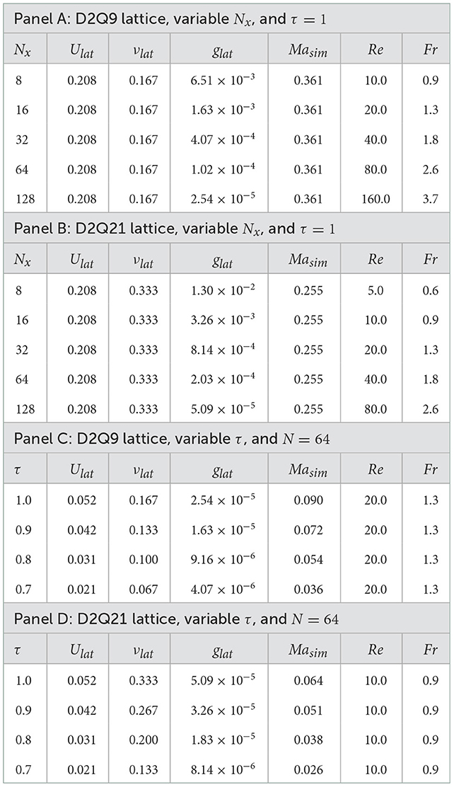
Table 2. Plane Poiseuille LBM parameters.
For D2Q9 lattice with CR = 0, all quantities ρ(x), 1(x), and 2(x) produced by the new method [4] for all resolutions Nx = 8, 16, 32, 64, 128 accurately reproduce the exact analytical solution (Equations 24, 25).
The Table 2B above details the LBM parameters we used for the D2Q21 lattice cases. For D2Q21 lattice with CR = 0 the new curvilinear algorithm [4] also converges well to the exact solution for all considered resolutions Nx = 8, 16, 32, 64, 128. As in the previous Couette flow case for D2Q21 we observe some very small influence of the boundary conditions.
In Figures 6A–7B below we present the numerical solution to the non-equidistant case with compression of cells with CR = 0.4. The results for ρ(x) and 2(x), for D2Q9 and CR = 0.4 are shown in Figures 6A, B below.
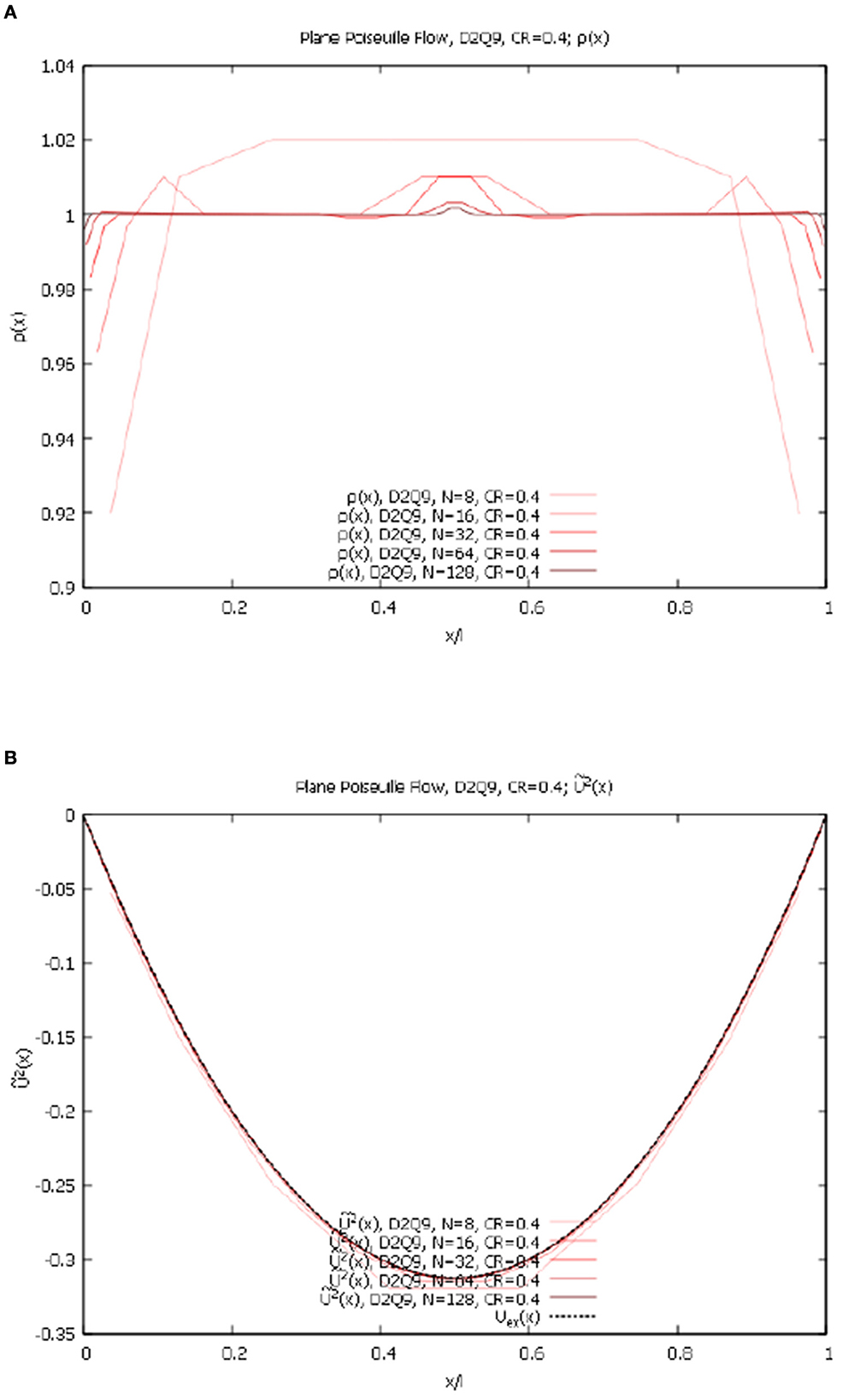
Figure 6. Plane Poiseuille flow, contracting grid, variable Nx, D2Q9 lattice. (A) ρ(x) for Nx = 8, 16, 32, 64, 128 and CR = 0.4. (B) 2(x) for Nx = 8, 16, 32, 64, 128 and CR = 0.4.
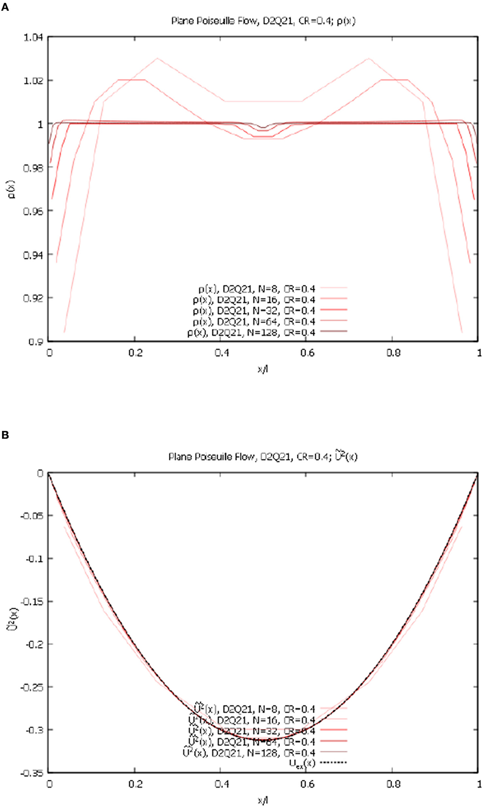
Figure 7. Plane Poiseuille flow, contracting grid, variable Nx, D2Q21 lattice. (A) ρ(x) for Nx = 8, 16, 32, 64, 128 and CR = 0.4. (B) 2(x) for Nx = 8, 16, 32, 64, 128 and CR = 0.4.
1 in this case is negligibly small for all resolutions. We again observe a very good convergence with the increase in resolution to the exact solution (Equations 24, 25). The results for ρ(x) and 2 for D2Q21 and CR = 0.4 are shown in Figures 7A, B below.
We again observe a very good convergence with the increase in resolution to the exact solution (Equations 24, 25). One can notice a better performance of the D2Q21 lattice in the middle of the domain than that of the D2Q9.
Let us now show the results of numerical model solutions for a fixed resolution N = 64 but variable τ = {1.0, 0.9, 0.8, 0.7} for both lattices D2Q9 and D2Q21. The corresponding LBM parameters for the D2Q9 lattice we used are shown in Table 2C above.
The agreement of numerical with the exact solution with no lattice compression CR = 0 was very good for both lattices D2Q9 and D2Q21 for all τ = {1.0, 0.9, 0.8, 0.7}. Below in Figures 8A, B we present the comparisons of numerical results with the exact solution for lattice D2Q9 with compression CR = 0.35 and τ = {1.0, 0.9, 0.8, 0.7}. We show variable τ cases on the same graphs, for the following quantities: , and .

Figure 8. Plane Poiseuille flow, contracting grid, variable τ for D2Q9 lattice. (A) for D2Q9, τ = 1.0, 0.9, 0.8, 0.7, and CR = 0.35. (B) for D2Q9, τ = 1.0, 0.9, 0.8, 0.7, and CR = 0.35.
The for D2Q9, τ = 1.0, 0.9, 0.8, 0.7, and CR = 0.35, are all equal to zero within double-precision accuracy and the for D2Q9, τ = 1.0, 0.9, 0.8, 0.7, and CR = 0.35 show very weak dependence on τ. As one can see, the new method [4] using the D2Q9 lattice with strong cell compression works well for various values of parameter τ.
The corresponding LBM parameters for the D2Q21 lattice we used are shown in Table 2D above. In Figures 9A, B below we present the numerical results for D2Q21 lattice.
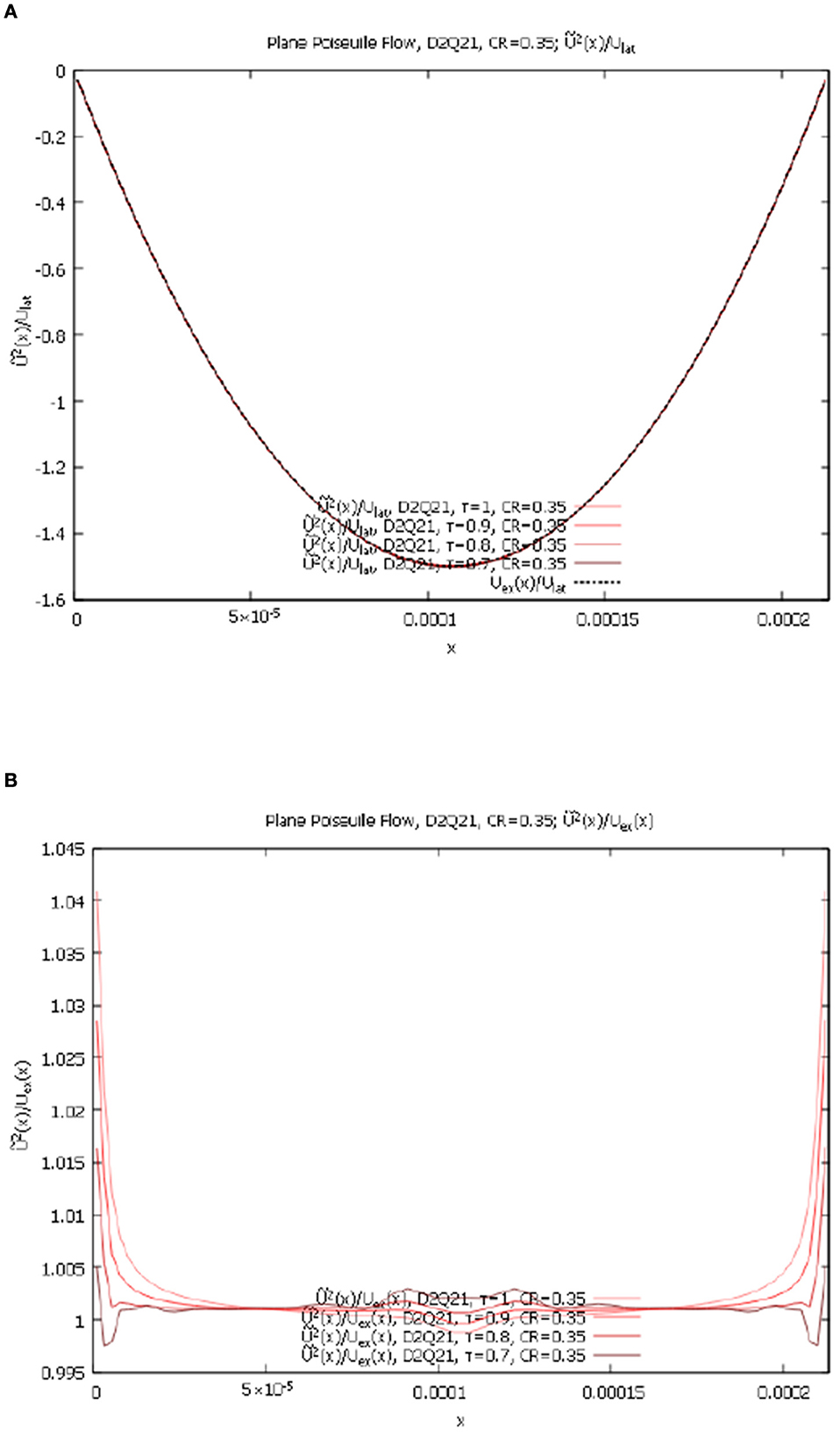
Figure 9. Plane Poiseuille flow, contracting grid, variable τ for D2Q21 lattice. (A) for D2Q21, τ = 1.0, 0.9, 0.8, 0.7, and CR = 0.35. (B) for D2Q21, τ = 1.0, 0.9, 0.8, 0.7, and CR = 0.35.
Similar to the D2Q9 case, the for D2Q21, τ = 1.0, 0.9, 0.8, 0.7, and CR = 0.35, are approximately equal to zero and the for D2Q21, τ = 1.0, 0.9, 0.8, 0.7, and CR = 0.35 show very weak dependence on τ. Here we observe that the new method [4] with strong compression also works well for various values of parameter τ.
To summarize, for these two planar geometry problems above, both D2Q9 and D2Q21 lattices provide adequate and comparable performance for cases with and without lattice compression. Let us now move on to problems with intrinsic curvilinearity.
This is also a well-known [18] naturally curvilinear problem with a closed-form exact solution, which fits very well for our purpose of validating the new method. This solution describes a stationary flow of viscous liquid between two infinite concentric vertical cylinders with radii R1 for the internal one and R2 for the external one, rotating with corresponding angular velocities Ω1 and Ω2. Here we will need the leading order in (Mach number) exact solution of the compressible Navier-Stokes equations.
For both of the circular problems considered here, we can introduce a measure of natural curvilinearity, a coefficient . If we keep the distance between cylinders R2 − R1 = const, then NCR = 1 corresponds to a previously considered planar case for R1 → +∞. Conversely, cases NCR ≫ 1 correspond to cases with strong natural curvilinearity. The Reynolds number for this problem was defined as . An example of geometry and the lattice with strong natural curvilinearity with NCR = 11 that we have used in the calculations is shown in Figure 1B.
The θ-component of the Navier-Stokes equations written in polar coordinates in our case of a stationary r-dependent, θ-directional flow is:
with the following solution:
Note that this classical solution has the following properties: it is a non-monotonic function of r for with an extremum at
and it is a monotone function outside of this interval.
Also, note that the above velocity profile has the same leading order behavior in small parameters for l = R2 − R1 and x = r − R1 as the exact planar Couette flow solution when both vertical planes are moving with velocities U1 = Ω1R1 and U2 = Ω2R2:
which for U1 = 0 reproduces the exact solution for the plane Couette flow Equation 21.
The radial component of the Navier-Stokes equation for a stationary r-dependent flow only in θ-direction, is:
which simplifies into the following 1-st order ODE:
The LBM formalism results in an expansion in powers of Ma number with the ideal gas law equation of state:
If we substitute this into the previous incompressible equation, we obtain the leading order in Ma ODE for density:
This defines the density behavior at the leading order in Ma:
where:
The integration constant can be determined using conservation of total mass:
which leads to:
where we denoted:
Thus the leading-order in Ma exact solution for density is:
We will need the above exact solution for velocity expressed in lattice units on the non-equidistant lattice:
where we denoted:
and similar to earlier definitions, is the average step in the radial direction. Similarly, the exact solution for density in lattice units on the non-equidistant lattice is:
where we denoted:
and
In both of our circular problems, we used the same method of choosing the azimuthal lattice size Nθ as a function of radial lattice size Nr, which was the following. Requiring that the lattice cells near r = R1 are approximately equilateral results in .
Obviously, such intrinsically curvilinear problems cannot be solved by a standard LBM even without radial lattice step contraction. Therefore, here we present the comparisons between D2Q9 and D2Q21 lattices without radial grid contraction for a case of strong natural curvilinearity NCR = 11. We have considered the case of Ω2 = 0 in the numerical solutions below.
The LBM parameters for the D2Q9 lattice we have used are presented in Table 3A, and the LBM parameters used for the D2Q21 lattice are presented in Table 3B.
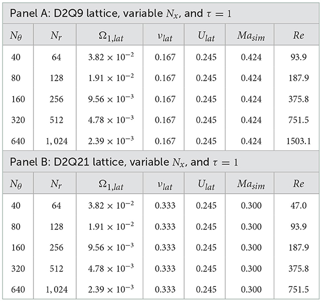
Table 3. Circular Couette LBM parameters.
In Figures 10A–C we present the numerical solutions for ρ(r), r(r), and θ(r) for resolutions Nr = 64, 128, 256, 512, and 1,024 for D2Q9 lattice. Note that in the cases below we only show ρ after the application of the "no flow" adjustment described above.
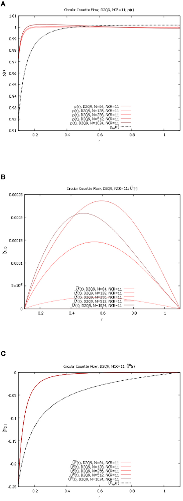
Figure 10. Circular Couette flow, NCR = 11, variable Nr, D2Q9 lattice. (A) ρ(r) for Nr = 64, 128, 256, 512, 1,024 and NCR = 11. (B) r(r) for Nr = 64, 128, 256, 512, 1,024 and NCR = 11. (C) θ(r) for Nr = 64, 128, 256, 512, 1,024 and NCR = 11.
In a drastic difference to the previously considered planar problems, we observe here that the D2Q9 lattice does not converge to the exact solutions (Equations 25, 31, 32, 34). This calls for exploring of the higher-order D2Q21 lattice.
Figures 11A–C present the numerical solutions for ρ(r), r(r), and θ(r) for resolutions Nr = 64, 128, 256, 512, and 1,024 for D2Q21 lattice, which possesses a higher degree of isotropy (see Appendix A).
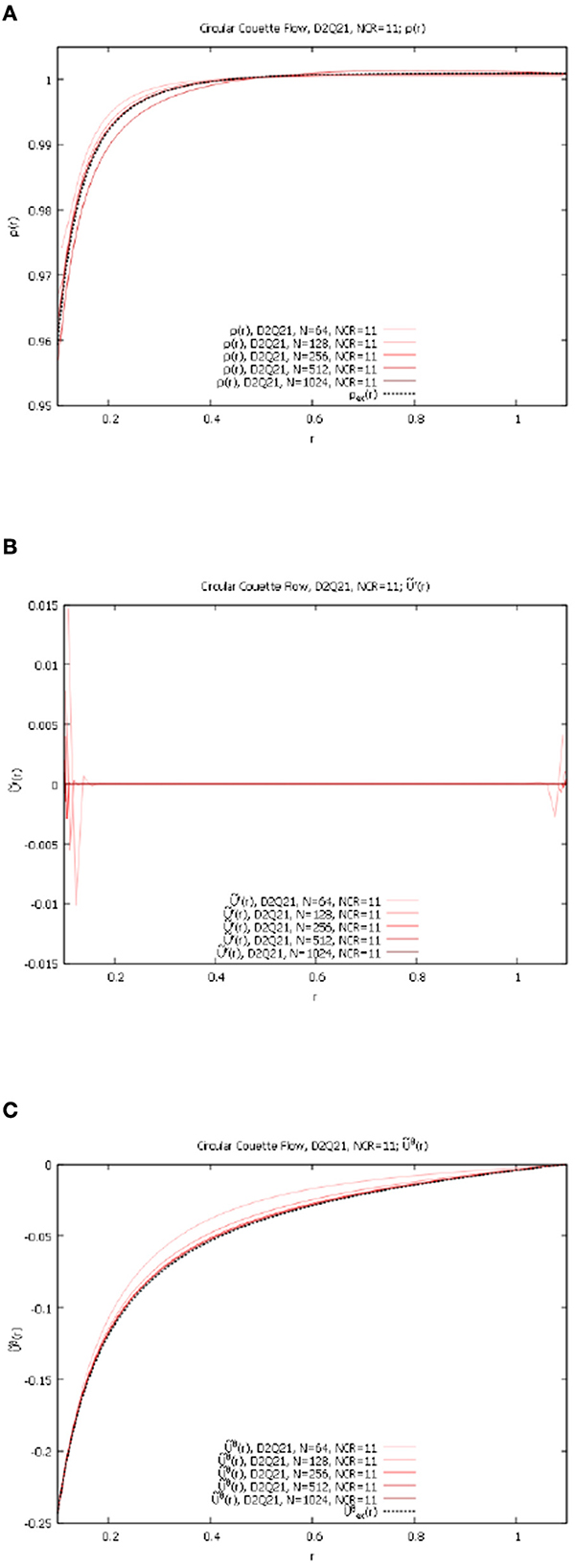
Figure 11. Circular Couette flow, NCR = 11, variable Nr, D2Q21 lattice. (A) ρ(r) for Nr = 64, 128, 256, 512, 1,024 and NCR = 11. (B) r(r) for Nr = 64, 128, 256, 512, 1,024 and NCR = 11. (C) θ(r) for Nr = 64, 128, 256, 512, 1,024, and NCR = 11.
Notice that unlike in the D2Q9 case, the implementation of the model based on the D2Q21 lattice does converge very well to the exact solutions (Equations 26, 31, 32, 34) with the increase in resolution. The more widely used D2Q9 lattice simply does not have sufficient isotropy to support the LBM on the curvilinear mesh.
Let us try to outline here the reasons for the importance of higher-order isotropy. As shown in Chen [4], the 6th-order isotropy is required to reproduce the Navier-Stokes equation in curvilinear coordinates. In particular, the 3-rd order tensor Qijk,eq will satisfy the 6th order isotropy condition given by the Equation (32) of Chen [4] for a specific choice of equilibrium distribution function , which requires the Hermite expansion up to 3rd-order, given by the Equation (33) of Chen [4]. Therefore, the 6th-order isotropy as defined in the last Equation (10) of Chen [4] is required in order to avoid discrete rotational artifacts.
Similar to the previous case, this is a naturally curvilinear problem with the same exact geometry, but it has a closed-form exact solution which in the limiting case of , such that R2 − R1 = const converges to the Plane Poiseuille flow considered above. For this problem, in addition to the Reynolds number , we can also define the Froude number as , with the average velocity obtained from the exact solution below.
This is a model problem that we at the present time can not connect to any physical situation but is useful for analyzes of numerical aspects associated with curvilinear LBM. We are not aware that this problem was considered before.
As is shown in Appendix D, a constant curvilinear second co-tangent component of the external “gravity” force g2 corresponds to the following external “gravity” component in polar coordinates:
Denote , then the θ-component of the external "gravity" force corresponds to the acceleration . Similarly to the previous section, in the particular case of stationary r-dependent and θ-directional flow in the presence of external force with acceleration , which is pushing the fluid in the clockwise azimuthal direction for α > 0, we get:
resulting in:
Here , is the kinematic viscosity, and the constants a and b determined from the no-slip boundary conditions uθ(R1) = uθ(R2) = 0:
The velocity profile given by the Equation (39) which starts and ends at 0 and has a minimum at:
One can also define the average velocity which can be used as a characteristic flow velocity for the specification of Reynolds and Froude numbers:
Note that the leading-order behavior of this curvilinear flow in the small parameters x, ϵ: , is:
where we denoted , which exactly corresponds to the plane Poiseuille flow in Cartesian coordinates (Equation 24).
The radial component of the Navier-Stokes equation Equation (28) with the equation of state given by the Equation (29) becomes
with the solution:
where:
and
Rewritten in lattice units,
As we have shown in the previous section, on non-equilateral grid systems the D2Q9 lattice cannot adequately reproduce the exact solutions in intrinsically curvilinear geometries due to the lack of 6-th order isotropy. Therefore, we will be only showing here the results for the D2Q21 lattice. We have again used the same case of strong intrinsic curvilinearity NCR = 11.
The Table 4 below lists the set of LBM parameters used for comparisons in this case:
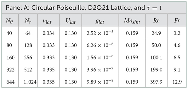
Table 4. Circular Poiseuille flow, D2Q21 lattice parameters, and τ = 1.
The numerical solutions for ρ(r), r(r) and θ(r) for resolutions Nr = 64, 128, 256, 512, and 1,024 for D2Q21 lattice are presented in Figures 12A–C.
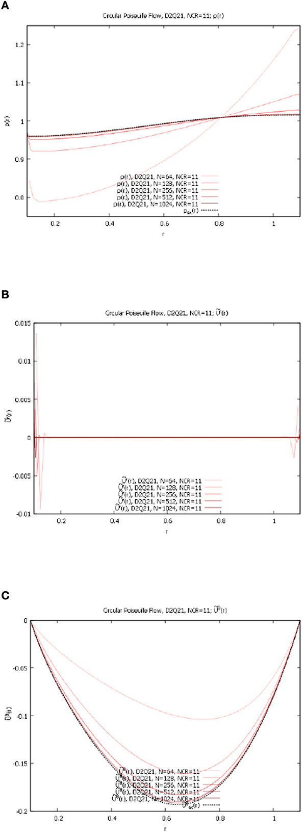
Figure 12. Circular Poiseuille flow, NCR = 11, variable Nr, D2Q21 lattice. (A) ρ(r) for Nr = 64, 128, 256, 512, 1,024 and NCR = 11. (B) r(r) for Nr = 64, 128, 256, 512, 1,024 and NCR = 11. (C) θ(r) for Nr = 64, 128, 256, 512, 1,024 and NCR = 11.
We again observe that the new fully curvilinear method [4] using D2Q21 converges very well to the exact solutions Equations (28, 39, 47, 49) with the increase in resolution.
A somewhat high number of grid points (such as Nr = 512 and higher for the Circular Poiseuille problem considered above) was required to get sufficient accuracy for the curvilinear cases. We do not see this however as a major obstacle to the practical implementation of the new method. The observed high-resolution requirement is partially due to some imperfections in the boundary condition algorithm. This paper is the first to numerically establish that the current curvilinear LBM is able to recover the Navier-Stokes hydrodynamics asymptotically. How to improve the rate of convergence with a lower number of grid points is a research topic for the future.
In this work, we have provided the first numerical tests of the novel volumetric curvilinear LBM method [4]. The accuracy and performance of the new method have been investigated and validated on a set of four 2D exactly solvable models: with and without the natural curvilinearity. The crucial importance of the isotropy requirement of at least 6th-order which requires at least D2Q21 lattice in 2D cases has also been demonstrated. We considered four 2-dimensional exactly solvable problems. For Cartesian lattice problems with possible grid compression, both D2Q9 and D2Q21 lattices give accurate results converging to the exact solutions for various values of . For truly curvilinear cases considered we have presented evidence that the 4th-order isotropy of D2Q9 is insufficient and the D2Q21 lattice with 6th-order isotropy is needed for convergence to the exact solution.
This illustration of the importance of moments' isotropy is very important. As it was stated in Chen [4], a certain set of moment isotropy constraints and normalization conditions must be satisfied in order to correctly recover the full Navier-Stokes equations [16, 19–22]. In wide practical use are the small stencil length LBM lattices, such as D2Q9, largely due to their simplicity of implementation, specifically for the boundary conditions. However, as we discuss in Appendix A, D2Q9 lattice satisfies the requirements of moments' isotropy only to the 4-th order. Only the D2Q21 lattice satisfies those conditions to the 6th-order.
The convergence to exact analytical solutions with the increase in resolution for various values of τ we have obtained is quite good for all cases considered using the D2Q21 lattice. However, the simpler D2Q9 lattice can still be used only for Cartesian geometry cases with 1-dimensional grid compression. The curvilinear LBM method [4], although somewhat slower than the standard LBM method due to its higher mathematical complexity, still keeps all the advantages of the classical LBM method, such as intrinsic parallelism, applicability to complex physics cases (such as multi-phase flows, etc.), and no numerical diffusion at the advection stage.
In order to perform our studies we have developed the generalized LBM boundary conditions of periodicity, no-slip, and moving wall types for the fully curvilinear geometry. We have additionally proposed a "no flow" adjustment procedure which helps to compensate for the effects of analytical finite-difference approximation for generalized basis vectors used in Chen [4].
We find our results to be very promising because, in our view, they open the much-needed way to expand the LBM method advantages to curvilinear geometries. The inability of the LBM method to adequately treat truly curvilinear cases and adaptive grids has been perceived as a weakness of LBM methods as compared to the classical finite-difference methods. In particular, such problems as adaptive grid compression into the boundary layer for high Reynolds number flows can possibly be addressed.
Much work remains to be done, such as studies of 3-dimensional flows, extension to turbulent flow, extensions to multi-phase and multi-component flows, development of higher-order LBM boundary conditions for curvilinear cases for lattices with wider stencils such as D2Q21, and many others.
The original contributions presented in the study are included in the article/Supplementary material, further inquiries can be directed to the corresponding author.
Based on the breakthrough theoretical work by HC (see: HC, Frontiers in Applied Mathematics and Statistics, 7:1–11, June 2021). AC has implemented the proposed model in four two-dimensional curvilinear problems with exact analytical solutions. Three of these problems are well-known and one of them has the exact solution developed by him in the paper. Important additional theoretical, analytical, and numerical contributions are made by RZ and IS. All authors contributed to the article and approved the submitted version.
AC, IS, RZ, and HC are employed by Dassault Systemes.
All claims expressed in this article are solely those of the authors and do not necessarily represent those of their affiliated organizations, or those of the publisher, the editors and the reviewers. Any product that may be evaluated in this article, or claim that may be made by its manufacturer, is not guaranteed or endorsed by the publisher.
The Supplementary Material for this article can be found online at: https://www.frontiersin.org/articles/10.3389/fams.2022.1066522/full#supplementary-material
1. Hudong C. Volumetric formulation of lattice Boltzmann method for fluid dynamics: basic concept. Phys Rev E. (1998) 58:3955–63. doi: 10.1103/PhysRevE.58.3955
2. Chen H, Filippova O, Hoch J, Molvig K, Shock R, Teixeira C, et al. Grid refinement in lattice Boltzmann methods based on volumetric formulation. Physica A Stat Mechits Appl. (2006) 362:158–67. doi: 10.1016/j.physa.2005.09.036
3. Chen H, Teixeira C, Molvig K. Realization of fluid boundary conditions via discrete Boltzmann dynamics. Int J Modern Phys C. (1998) 9:1281–92. doi: 10.1142/S0129183198001151
4. Chen H. Volumetric lattice Boltzmann models in general curvilinear coordinates: theoretical formulation. Front Appl Math Stat. (2021) 7:691582. doi: 10.3389/fams.2021.691582
5. He X, Luo L, Dembo M. Some progress in lattice Boltzmann method, part 1. non-uniform mesh grids. J Comput Phys. (1996) 129:357–63. doi: 10.1006/jcph.1996.0255
6. Barraza JAR, Dieterding R. Towards a generalised Lattice-Boltzmann method for aerodynamic simulations. J Comput Sci. (2019) 45:1–12. doi: 10.1016/j.jocs.2020.101182
7. Aris R. Vectors, Tensors, and the Basic Equations of Fluid Mechanics. Dover, MA: Dover Publications (1962).
8. Mendoza M, Debus JD, Succi S, Herrmann HJ. Lattice kinetic scheme for generalized coordinates and curved spaces. Intl J Mod Phys C. (2014) 25:1441001. doi: 10.1142/S0129183114410010
9. Debus JD, Mendoza M, Herrmann HJ. Dean instability in double-curved channels. Phys Rev E. (2014) 90:053308. doi: 10.1103/PhysRevE.90.053308
10. Debus JD, Mendoza M, Succi S, Herrmann HJ. Poiseuille flow in curved spaces. Phys Rev E. (2016) 92:043316. doi: 10.1103/PhysRevE.93.043316
11. Frisch U, D'Humieres D, Hasslacher B, Lallemand P, Pomeau Y, Rivet JP. Lattice gas hydrodynamics in two and three dimensions. Complex Syst. (1987) 1:649–707.
12. Chen S, Chen H, Martinez D, Matthaeus W. Lattice Boltzmann model for simulation of magnetohydrodynamics. Phys Rev Lett. (1991) 67:3776–9. doi: 10.1103/PhysRevLett.67.3776
13. Chen H, Chen S, Matthaeus W. Recovery of the Navier-Stokes equations using a lattice-gas Boltzmann method. PhysRev A. (1992) 45:5339–42. doi: 10.1103/PhysRevA.45.R5339
14. Benzi R, Succi S, Vergassola M. The lattice Boltzmann equation: theory and applications. Phys Rep. (1992) 222:145–97. doi: 10.1016/0370-1573(92)90090-M
15. Qian Y, D'Humieres D, Lallemand P. Lattice BGK models for Navier-Stokes equation. Europhys Lett. (1992) 17:479–84. doi: 10.1209/0295-5075/17/6/001
16. Chen H, Teixeira C, Molvig K. Digital physics approach to computational fluid dynamics: some basic theoretical features. Int J Modern Phys C. (1997) 8:675–84. doi: 10.1142/S0129183197000576
17. Bhatnagar P, Gross E, Krook M. A model for collision processes in gases. I. Small amplitude processes in charged and neutral one-component systems. Phys Rev. (1954) 94:511–25. doi: 10.1103/PhysRev.94.511
19. Chen H, Goldhirsch I, Orszag SA. Discrete rotational symmetry, moment isotropy, and higher order lattice boltzmann models. J Sci Comp. (2008) 34:87–112. doi: 10.1007/s10915-007-9159-3
20. Shan X, Yuan X, Chen H. Kinetic theory representation of hydrodynamics: a way beyond the Navier-Stokes equation. J Fluid Mech. (2006) 550:413–41. doi: 10.1017/S0022112005008153
21. Chen H, Zhang R, Staroselsky I, Jhon M. Recovery of full rotational invariance in lattice boltzmann formulations for high knudsen number flows. Physica A Stat Mechits Appl. (2006) 362:125–31. doi: 10.1016/j.physa.2005.09.008
Keywords: Lattice Boltzmann Method, generalized coordinates, Chapman–Enskog theory, Boltzmann equation, numerical methods, fluid mechanics
Citation: Chekhlov A, Staroselsky I, Zhang R and Chen H (2023) Lattice Boltzmann model in general curvilinear coordinates applied to exactly solvable 2D flow problems. Front. Appl. Math. Stat. 8:1066522. doi: 10.3389/fams.2022.1066522
Received: 11 October 2022; Accepted: 06 December 2022;
Published: 11 January 2023.
Edited by:
Snezhana I. Abarzhi, University of Western Australia, AustraliaReviewed by:
Tulin Kaman, University of Arkansas, United StatesCopyright © 2023 Chekhlov, Staroselsky, Zhang and Chen. This is an open-access article distributed under the terms of the Creative Commons Attribution License (CC BY). The use, distribution or reproduction in other forums is permitted, provided the original author(s) and the copyright owner(s) are credited and that the original publication in this journal is cited, in accordance with accepted academic practice. No use, distribution or reproduction is permitted which does not comply with these terms.
*Correspondence: Alexei Chekhlov,  YWxleGVpLmNoZWtobG92QDNkcy5jb20=
Disclaimer: All claims expressed in this article are solely those of the authors and do not necessarily represent those of their affiliated organizations, or those of the publisher, the editors and the reviewers. Any product that may be evaluated in this article or claim that may be made by its manufacturer is not guaranteed or endorsed by the publisher.
Research integrity at Frontiers
Learn more about the work of our research integrity team to safeguard the quality of each article we publish.