A multi-cycle inventory control model for deteriorating items with partial backlogging under trade credit

The finite horizon should be considered for products with a limited lifecycle. To introduce this possibility, multiple orders and partial backlogging policies are established under trade credit in an inventory model, where demand is a time-varying function and the backlogging rate is a decreasing function about a customer's waiting time. This paper presents lemmas and theories to determine optimal replenishment time and backlogging time to maximize total profit for the retailer. A search algorithm to solve the optimal order strategy is proven based on the theoretical results. Numerical examples are presented, and the optimal order strategy is obtained. A sensitivity analysis of the main parameters is carried out. The effects of total profit on the main parameter of trade credit are analyzed from both macroscopic and microscopic perspectives.

Introduction

With increasing uncertainties about demand, shortages are inevitable. Uncertain factors include the situation of demand exceeding supply. For products that are favored, some customers are willing to wait for the next delivery. As a result, the enterprise adopts the partial backlogging strategy accordingly. Concurrently, to improve customer service and reduce unnecessary inventory backlog, the retailer takes a small-batch and multi-batch order strategy in the finite planning horizon, utilizing smooth traffic and convenient information channel.

Uncertainties have penetrated real life and many interdisciplinary fields, such as ecology [1], computer science [2], and nonlinear dynamics [3]. To deal with these uncertainties, a great deal of feasible approaches were proposed and put into practical application, for instance, fuzzy model [4] and signal filtering [5].

On one hand, shortages are allowed and the part of low demand is canceled at the end of the sales period, that is, a retailer deletes the part with a low profit margin and improves the overall profit margin to achieve the sales goal. At the same time, scholars have different methods for different shortage situations, which can be roughly divided into three situations: the first is no replenishment for shortage, the second is complete backlogging for shortage, and the third is partially delayed replenishment. The three situations have their own scope of application. Such as, the reason for not replenishing out of stock may be that customers are unwilling to wait or the product has strong timeliness [6]. While completely delaying replenishment if customers are willing to wait or the product is particularly favored by customers [7]. Among them, some of the reasons for the delay in supply may lie between the abovementioned two situations because some customers are prepared to wait [8].

On the other hand, in the universal inventory model, the planning period is infinite, and scholars mainly consider the optimal solution of the ordering strategy of the single-cycle model [9]. However, the retailer's actual sales are not only single cycle or repeating most cycles indefinitely. Therefore, the optimal ordering strategy of each sales cycle should be gradually decided in the planning period according to the actual situation, so that the retailer can achieve the goal of maximum profit in the planning period [10].

To sum up, the main contribution of this paper is given in the following three aspects. Firstly, the trade credit strategy and partial trade credit replenishment were introduced in the limited planning period and the corresponding inventory model was established. Secondly, in the process of classification discussion, the optimal ordering strategy is deduced to solve each case, and the existence and uniqueness of the optimal solution are proven. Thirdly, according to the theoretical results and corresponding algorithms, the optimal solution of each sales cycle is solved gradually until the end of the planning period.

The remainder of this paper is outlined as follows. The literature is retrospect in section “ Literature review”. Section “Notation and assumptions” presents assumptions and notations of the model. The model is established in section “Model formulation”, and the calculation process is shown about the retailer's revenue and cost under different situations. In section “Theoretical results and optimal solutions”, the optimal solution of the model is deduced and the algorithm is given according to the theorem. Section “Numerical example” describes the numerical simulation and sensitivity analysis of the main parameters to prove the validity of the model. Based on the theory and numerical examples, Section “Conclusion” summarizes the management enlightenment of this paper and future research directions.

Literature review

Combined with the research theme of this paper, the literature review is carried out from the three aspects: trade credit in an inventory model, finite horizon research, and shortages and backlogging.

Trade credit in an inventory model

To increase market share and enhance market competitiveness, the supplier allows the retailer to delay the payment, namely, trade credit. In the case of the sale price being equal to the order price, Goyal [11] first introduced trade credit into the classical economic order quantity (EOQ) model. Then, Ouyang et al. [12] constructed the model closer to the actual market by modifying four assumptions according to the classical model of Goyal [11]: (1) the retailer's selling price per unit is significantly higher than per unit purchase price; (2) the interest rate charged by a bank is not necessarily higher than the retailer's investment return rate; (3) many items such as fruits and vegetables deteriorate continuously, and (4) the supplier may offer a partially permissible delay in payments even if the order quantity is less than the predetermined value. The trade credit policy is a strategy stimulating demand, but a certain risk exists. Therefore, considering their own interests, the supplier provides the trade credit policy through some restrictive conditions, for example, the credit period is associated with the order quantity with two cases comprising complete credit and partial credit.

The full trade credit means that the supplier will provide the trade credit policy as long as the retailer's order quantity arrives in the preset values, otherwise the retailer must pay all the payments immediately, as mentioned by Chung et al. [13], Chung and Liao [14], Chung and Liao [15], Kreng and Tan [16], and Ouyang et al. [17]. Yu [18] proposed an inventory model for deteriorating and backlogging under a two-warehouse system. The partial trade credit means that the retailer first pays a certain percentage of payment and the remaining payments are paid through trade credit strategy when the order quantity is less than preset values, otherwise the retailer can enjoy full trade credit. Nonetheless, Yung-Fu [9] and Chen et al. [19] extended the full credit inventory model to partial credit to render the inventory model closer to the real market. Tiwari et al. [20] built an EOQ model with partial trade credit for deteriorating items under complete backlogging. Xu et al. [21] considered the trapezoidal-type demand with warehouse mode selection under trade credit.

As discussed earlier, a single-level and two-level trade credit inventory models were built for exponentially deteriorating items by Chang et al. [22]. Tiwari et al. [23] formulated a two-level partial trade credit model for deteriorating items with partial backlogging. Vandana and Kaur [24] presented an integrated inventory model with a two-level trade credit under stochastic demand. Zou and Tian [25] discovered that offering a two-level trade credit contract will increase the retailer's total cost and reduce the retailer's early payment fraction through the model.

Finite horizon research

All the abovementioned inventory models with credit payment for a single cycle in the infinite horizon were decided as the optimal replenishment policies. However, most items have a lifecycle, based on the item's demand, the finite horizon has been divided into equal period or unequal period in the actual market. Panda et al. [26] introduced an inventory model for deteriorating and seasonal items with no shortages over the finite horizon, the maximum objective function of the model was calculated through a search algorithm and Newton–Raphson for the equations. Dey et al. [27] presented an inventory model with two-warehouses in the basal model, where the demand rate is an inverse function. Dye [10] established an inventory model with the equal period and time-varying deterioration rate under a dual function of the demand rate about time and price, which decided the optimal replenishment number and the optimal sale price. Lin et al. [28] proposed an inventory model with production rate depending on the demand rate and the inventory level for practitioners with a finite planning horizon. Palanivel et al. [29] complemented the two-warehouse in the past model. Udayakumar and Geetha [30] discussed two cases of no shortage and partial backlogging under trade credit. Pramanik and Maiti [31] obtained the optimal solution of the mode through artificial bee colony (ABC) and genetic algorithm (GA) under two-level partial trade credit. Xu et al. [32] introduced a supply chain optimization problem with selling price-dependent demand. In the abovementioned eight models where Panda et al. [26] and Pramanik and Maiti [31] built the unequal cycle inventory models, the rest of them were equal cycle models.

Shortages and backlogging

Shortages are not allowed in the classical EOQ models. However, a shortage exists in the actual market. The ways of treating shortages can be roughly divided into three types: shortages allowed and no backlogging; shortages allowed and fully backlogged; and shortages allowed and partially backlogged.

First, comparing with the optimal solution for traditional replenishment policies, Goyal et al. [6] extended no shortage to shortage and no backlogging.

Second, Kar et al. [7] complement the shortcomings of Goyal et al.'s [6] mode and assumed complete backlogging. Simultaneously, Jaggi et al. [33], Hui-Ling [34], and Jaggi et al. [35] considered inflation, two warehouses, and trade credit under full backlogging. San-José et al. [36] given an EOQ model with price- and time-dependent demand, Nath and Sen [37] expanded Nath and Sen's model with non-instantaneous deterioration. Sicilia et al. [38] extended the newsvendor model for stochastic demands.

Third, shortages allowed and partially backlogged are not only in accordance with the rule of the market but also satisfy customer needs. Based on the original model of Hui-Ling [34], the partially backlogged rate about the customer's waiting time was added by Hui-Ling [39]. To further improve the model, Yang and Chang [40] introduced trade credit into the model. Sana [8] assumed that the backlogging rate is an inverse proportional function about the waiting time and the deterioration rate of products is a linear function about quality guarantee period. Hsieh and Dye [41] established an inventory model with partial backlogging and decided the optimal replenishment number and sales prices, where the demand rate is a binary function about the time and sale price. Khan et al. [42] proposed an inventory model for non-instantaneous deteriorating items with a fixed backlogging rate and two warehouses. Sumon and Bibhas [43] assumed that the backlogging rate was a binary function about a customer's waiting time and an item's selling price. Soni and Suthar [44] supposed that the demand rate function is a negative and positive exponential effect of price and promotional effort. Rana et al. [45] developed an EOQ mode for optimal dispatching policies under inflation and partial backlogging. Among the models mentioned above with backlogging, Kar et al. [7] and Hsieh and Dye [41] studied the equal cycle problem in the finite planning horizon. The advancements in this paper related to the existing literature are presented in Table 1.

TABLE 1

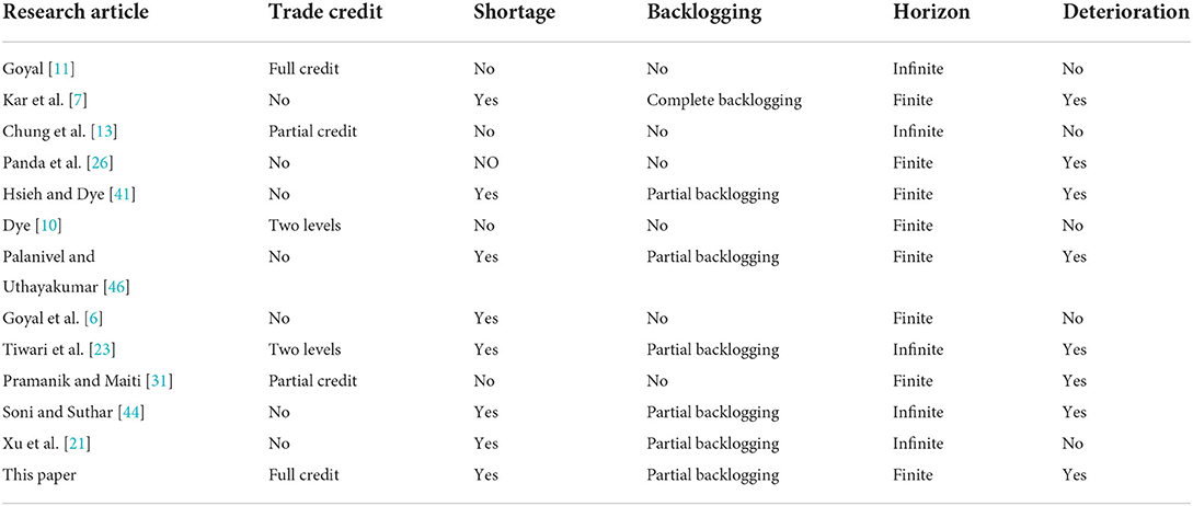
Table 1. Summary of some related literature studies with major assumptions.

In this paper, a multi-order problem for deteriorating items with an unequal period and partial backlogging is studied under trade credit. Supposing that the demand rate is an increasing exponential function, and the backlogging rate is a decreasing function about the waiting time, an inventory model that regarded the retailer's profit as the objective is established. A corresponding search algorithm for the order strategy is designed, and the optimality of every search step is proven. Concurrently, a numerical example is presented, and the sensitivity analysis of the main parameters is given.

Notation and assumptions

The following notation and assumptions are used in this paper.

Notations

p: the selling price per unit.

c₀: the purchasing cost per unit.

h: the holding cost per unit time excluding the capital cost.

c₁: backlogging cost per unit time.

c₂: opportunity cost per unit of lost sale.

t_i: the (i + 1)th replenishment time.

s_i: the time when the inventory level reaches 0 in the ith cycle.

T_i: the ith replenishment cycle.

I_i(t): the ith inventory level at time t ∈ [t_i−1, s_i] ∪ [s_i, t_i].

q_i: the order quantity of the ith replenishment cycle.

θ: the parameter of the deterioration rate of the stock.

I_e: the interest rate earned per unit of time.

I_c: the interest rate charged per unit of time.

M: the length of the trade credit period.

Assumptions

(1) Time horizon is finite and is of length H.

(2) Selling price is greater than purchasing cost, that is, p > c₀.

(3) The product's demand rate is a time-varying function with an exponential form, if $D(t)=D_0{e}^{\lambda t}$ is an increasing function; if $D(t)=D_0{e}^{\lambda (H-t)}$is a non-negative decreasing function, where D₀ > 0, λ > 0.

(4) Instantaneous replenishment: the lead time is 0. Shortages are allowed and partially backlogged for the next replenishment, the backlogging rate is a decreasing function, β(t) = e^−δt, δ > 0, where t is the waiting time of a customer.

(5) The number of replenishments is m in the finite time horizon, which satisfies the relation t_i−1 < s_i ≤ t_i, i = 1, ⋯, m.

(6) During the trade credit period [t_i−1, M + t_i−1], the account is not settled and the sales revenue is deposited in an interest-bearing account. At the end of the period, the retailer pays off all units bought and starts to pay the capital opportunity cost for the products in stock.

Model formulation

Under the abovementioned notation and assumptions, the inventory level I_i(t) of the ith cycle is described by

$\begin{array}{l}\frac{d{I}_i(t)}{dt}=-\theta I_i(t)-D(t)\begin{array}{cc},& t_{i-1}\le t\le s_i\end{array}.\end{array}$

With the boundary condition I_i(s_i) = 0, we have $I_i(t)={\int }_t^{s_i}{e}^{\theta (x-t)}D(x)dx.$

The inventory level I_i(t) at time t ∈ [s_i, t_i] of the ith cycle is described by

$\begin{array}{l}\frac{d{I}_i(t)}{dt}=-\beta (t_i-t)D(t)\begin{array}{cc},& s_i\le t\le t_i\end{array}.\end{array}$

With the boundary condition I_i(s_i) = 0, we have $I_i(t)=-{\int }_{s_i}^t{e}^{-\delta (t_i-x)}D(x)dx\begin{array}{cc},& s_i\le t\le t_i\end{array}.$

Given that Q_i = I_i(t_i−1) + (−I_i(t_i)), the ordering quantity of the ith cycle is

$\begin{array}{l}{Q}_i={\displaystyle {\int }_{t_{i-1}}^{s_i}}{e}^{\theta (x-t_{i-1})}D(x)dx+{\displaystyle {\int }_{s_i}^{t_i}}{e}^{-\delta (t_i-x)}D(x)dx.\end{array}$

The retailer's profit comprises the following components:

(a) The sales revenue: $P_i=p({\int }_{t_{i-1}}^{s_i}D(x)dx+{\int }_{s_i}^{t_i}{e}^{-\delta (t_i-x)}D(x)dx)$.

(b) The purchasing cost: $C_i=c_0{Q}_i=c_0({\int }_{t_{i-1}}^{s_i}{e}^{\theta (x-t_{i-1})}D(x)dx+{\int }_{s_i}^{t_i}{e}^{-\delta (t_i-x)}D(x)dx)$.

(c) The holding cost: $H_i=h{\int }_{t_{i-1}}^{s_i}{I}_i(t)dt=h{\theta }^{-1}{\int }_{t_{i-1}}^{s_i}(e^{\theta (x-t_{i-1})}-1)D(x)dx$.

(d) The shortage cost: $S_i=c_1{\int }_{s_i}^{t_i}\left[-I_i(t)\right]dt=c_1{\int }_{s_i}^{t_i}(t_i-x)e^{-\delta (t_i-x)}D(x)dx$.

(e) The lost sale cost: $O_i=c_2{\int }_{s_i}^{t_i}(1-e^{-\delta (t_i-x)})D(x)dx$.

(f) The interest earned IE_i and interest charged IC_i. Two cases are considered as follows (see Figure 1):

FIGURE 1

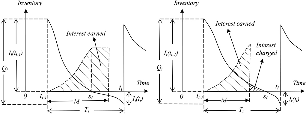
Figure 1. Interest earned and charged for s_i − t_i−1 < M or s_i − t_i−1 ≥ M.

Case 1: s_i − t_i−1 < M.

$\begin{array}{l}\text{I}{\text{E}}_{i1}=p{I}_e{\displaystyle {\int }_{t_{i-1}}^{s_i}}(M+t_{i-1}-x)D(x)dx,\text{I}{\text{C}}_{i1}=0.\end{array}$

Case 2: s_i − t_i−1 ≥ M.

$\begin{array}{l}\hfill \text{I}{\text{E}}_{i2}=p{I}_e{\displaystyle {\int }_{t_{i-1}}^{M+t_{i-1}}}(M+t_{i-1}-x)D(x)dx,\\ I{C}_{i2}=c_0{I}_c{\theta }^{-1}{\displaystyle {\int }_{M+t_{i-1}}^{s_i}}D(x)(e^{\theta (x-M-t_{i-1})}-1)dx.\end{array}$

Therefore, the retailer's profit is defined in the interval (t_i−1, H] as follows:

${\pi }_i(s_i,t_i)=\{\begin{array}{l}{\pi }_{i1}(s_i,t_i)\begin{array}{ll},\hfill & s_i<M+t_{i-1};\hfill \end{array}\hfill \\ {\pi }_{i2}(s_i,t_i)\begin{array}{ll},\hfill & s_i\ge M+t_{i-1}.\hfill \end{array}\hfill \end{array}$

where ${\pi }_{ij}(s_i,t_i)=P_i-C_i-H_i-S_i-O_i+\mathrm{\text{I}}{\mathrm{\text{E}}}_{ij}-\mathrm{\text{I}}{\mathrm{\text{C}}}_{ij}\begin{array}{cc},& j=1,2.\end{array}$

$\begin{array}{l}{\pi }_{i1}(s_i,t_i)=(p+h{\theta }^{-1}-c_2){\displaystyle {\int }_{t_{i-1}}^{s_i}}D(x)dx\\ +{\displaystyle {\int }_{s_i}^{t_i}}\left[p-c_0+c_2-c_1(t_i-x)\right]e^{-\delta (t_i-x)}D(x)dx\\ -(c_0+h{\theta }^{-1}){\displaystyle {\int }_{t_{i-1}}^{s_i}}{e}^{\theta (x-t_{i-1})}D(x)dx\\ +p{I}_e{\displaystyle {\int }_{t_{i-1}}^{s_i}}(M+t_{i-1}-x)D(x)dx,\end{array}$

$\begin{array}{l}{\pi }_{i2}(s_i,t_i)=(p+h{\theta }^{-1}-c_2){\displaystyle {\int }_{t_{i-1}}^{s_i}}D(x)dx\\ +{\displaystyle {\int }_{s_i}^{t_i}}\left[(p-c_0+c_2)-c_1(t_i-x)\right]e^{-\delta (t_i-x)}D(x)dx\\ -(c_0+h{\theta }^{-1}){\displaystyle {\int }_{t_{i-1}}^{s_i}}{e}^{\theta (x-t_{i-1})}D(x)dx\\ +p{I}_e{\displaystyle {\int }_{t_{i-1}}^{M+t_{i-1}}}(M+t_{i-1}-x)D(x)dx\\ -c_0{I}_c{\theta }^{-1}{\displaystyle {\int }_{M+t_{i-1}}^{s_i}}(e^{\theta (x-M-t_{i-1})}-1)D(x)dx.\end{array}$

This paper aims to determine the optimal replenishment time s_i and the optimal replenishment time t_i with t_i−1 < s_i ≤ t_i, i = 1, …, m, t₀ = 0, t_m = H such that the retailer's profit,

$\begin{array}{l}\pi (s_1,t_1,\cdots ,s_m,t_m)={\displaystyle {\sum }_{i=1}^m}{\pi }_i(s_i,t_i),\end{array}$

is maximized in the finite horizon H. The corresponding mathematical model is

$(P)\{\begin{array}{ll}\max \hfill & \pi (s_1,t_1,\cdots ,s_m,t_m)\hfill \\ s.t.\hfill & t_{i-1}<s_i\le t_i,i=1,\cdots ,m;\hfill \\ \hfill & \begin{array}{l}{t}_0=0,t_m=H\hfill \end{array}.\hfill \end{array}$

Theoretical results and optimal solutions

Considering the complexity of the objective function, we adopt the following method to solve this model: assuming that t₀, …, t_i−1 are known, we search s_i and t_i, with s_i ≤ t_i in the interval (t_i−1, H] to maximize π_i(s_i, t_i), i = 1, ⋯ , m. Therefore, first, we search t_i (denoted by t_i = t(s_i)) in the interval [s_i, H]to maximize π_i(s_i, t_i) for any given s_i, then we search s_i with s_i > t_i−1 (denoted by $s_i^{*}$) to maximize π_i(s_i, t(s_i)), thus $(s_i^{*},t_i^{*})$ is the solution, where $t_i^{*}=t(s_i^{*}).$

For convenience, we denote t_i and π_i(t_i) as t and π_i(t), respectively. Based on the relation between s_i − t_i−1 and M, two cases are discussed.

Sales cycle less than the trade credit, namely, s_i − t_i−1 < M

Now the retailer's profit function is π_i1(s, t). Taking the derivative of π_i1(s, t) with respect to t will give

$\begin{array}{ll}\frac{\partial {\pi }_{i1}(s,t)}{\partial t}={(\delta +\lambda )}^{-2}D(t)E(s,t).& (1)\end{array}$

where

$\begin{array}{l}E(s,t)={\left(\delta +\lambda \right)}^2(p-c_0)-\delta (\delta +\lambda )(p-c_0+c_2)-c_1\lambda \\ +e^{(\delta +\lambda )(s-t)}[\delta (\delta +\lambda )(p-c_0+c_2)\\ -c_1\left(\delta (\delta +\lambda )(t-s)-\lambda \right)].& (2)\end{array}$

Namely, x = t − s, from Equation 2, it follows that

$\begin{array}{l}E(x)={\left(\delta +\lambda \right)}^2(p-c_0)-\delta (\delta +\lambda )(p-c_0+c_2)-c_1\lambda \\ +e^{-(\delta +\lambda )x}[\delta (\delta +\lambda )(p-c_0+c_2)\\ +c_1\lambda -c_1\delta (\delta +\lambda )x].& (3)\end{array}$

Taking the derivative of E(x) will give

$\begin{array}{ll}{E}^{\prime }(x)=-{(\delta +\lambda )}^2{e}^{-(\delta +\lambda )x}\left[\delta (p-c_0+c_2)+c_1(1-\delta x)\right].& (4)\end{array}$

From E′(x) = 0, it follows that

$\begin{array}{ll}{x}_0=\left[\delta (p-c_0+c_2)+c_1\right]/c_1\delta .& (5)\end{array}$

Given that p > c₀, hence x₀ > 0.

Lemma 1: Let t¹ is the maximum point of π_i1(s, t) on [s, H] for any given s. Then, the following conclusions are obtained:

(i) If E(x₀) ≥ 0, or E(x₀) < 0 and H < x₁ + s, then t¹ = H.

(ii) If E(x₀) < 0 and H ≥ x₁ + s, then t¹ = x₁ + s, where x₀ is computed by Equation 5, x₁ is a unique solution of equation E(x) = 0 in the interval [0, x₀].

Proof. From Equation 4, we obtain that x₀ is the minimum point of E(x), because if x < x₀, then E′(x) < 0, hence E(x) is a decreasing function, if x > x₀, then E′(x) > 0, hence E(x) is an increasing function.

(1) If E(x₀) ≥ 0, then E(x) ≥ 0 for any given x > 0. From Equation 1, it follows that ∂π_i1(s, t)/∂t > 0 for any given s and t. Given that t ≤ H, hence π_i1(s, t) obtains the maximum at t = H, which says t¹ = H.

(2) If E(x₀) < 0, because of $E(0)={(\delta +\lambda )}^2(p-c_0)>0$ and E′(x) < 0, based on the intermediate value theorem, the unique solution x₁ exists in the interval (0, x₀), which allows E(x₁) = 0 and only if 0 < x < x₁, then E(x) > 0, if x₁ < x < x₀, E(x) < 0. According to x = t − s and Equation 1, if s < t < x₁ + s, ∂π_i1(s, t)/∂t > 0; if t = x₁ + s, ∂π_i1(s, t)/∂t = 0; if x₁ + s < t < x₀ + s, then ∂π_i1(s, t)/∂t < 0. Hence, if x₁ + s > H, when t ∈ [s, H], t ≤ H < x₁ + s, hence ∂π_i1(s, t)/∂t > 0, then the maximum point of π_i1(s, t) is H in the interval t ∈ [s, H], which says t¹ = H. If x₁ + s ≤ H, then the maximum point of π_i1(s, t) is x₁ + s, which says $t^1=x_1+s$.

Lemma 1 reveals that t¹ is a function about s. Motivated by t = t¹(s), we obtain ${\pi }_{i1}(s,t^1(s))$. Next, we search s ∈ [t_i−1, H] to let ${\pi }_{i1}(s,t^1(s))$ acquire the maximum. Based on Lemma 1, three cases are discussed as follows:

(a) E(x₀) ≥ 0. Now, t¹(s) = H, taking the derivative of ${\pi }_{i1}(s,t^1(s))$ will give

$\begin{array}{ll}\frac{d{\pi }_{i1}(s,t^1(s))}{ds}=D(s)F_i(s).& (6)\end{array}$

where

$\begin{array}{l}{F}_i(s)=(p-c_0+c_2)\left[1-e^{-\delta (H-s)}\right]+c_1(H-s)e^{-\delta (H-s)}\\ +(c_0+h{\theta }^{-1})(1-e^{\theta (s-t_{i-1})})+p{I}_e(M+t_{i-1}-s).\end{array}$

Given that t_i−1 ≤ s ≤ t ≤ H and s_i < M + t_i−1, then t_i−1 ≤ s ≤ a_i, where a_i = min{M + t_i−1, H},. We summarize our finding for ${\pi }_{i1}(s,t^1(s))$ in Lemma 2.

Lemma 2: Let s¹ be the maximum point of ${\pi }_{i1}(s,t^1(s))$ on [t_i−1, a_i]. Then, the following conclusions are obtained:

(i) If F_i(a_i) ≥ 0, then $s^1=a_i$.

(ii) If F_i(a_i) < 0, then $s^1={s^{\prime }}_0$, where ${s^{\prime }}_0$ is a unique solution for F_i(s) = 0 in the interval [t_i−1, a_i].

Proof. Taking the derivative of F_i(s) will give

$\begin{array}{l}{F_i}^{\prime }(s)=-\left\{\delta (p-c_0+c_2)+c_1\left[1+\delta (H-s)\right]\right\}{e}^{-\delta (H-s)}\\ -(\theta c_0+h)e^{\theta (s-t_{i-1})}-p{I}_e.\end{array}$

Then ${F^{\prime }}_i(s)<0,$ hence F_i(s) is a decreasing function about s.

If F_i(a_i) ≥ 0, based on $F_i^{\prime }(s)<0,$ F_i(s) ≥ 0, t_i−1 ≤ s ≤ a_i, from Equation 6, $d{\pi }_{i1}(s,t^1(s))/ds\ge 0,$ hence $s^1=a_i.$

If F_i(a_i) < 0, from p > c₀ and t_i−1 ≤ H, it follows that

$\begin{array}{l}{F}_i(t_{i-1})=(p-c_0+c_2)[1-e^{-\delta (H-t_{i-1})}]\\ +c_1(H-t_{i-1})e^{-\delta (H-t_{i-1})}+p{I}_{e}M.\end{array}$

Given that F_i(t_i−1) > 0, equation F_i(s) = 0 holds a unique solution (denoted by ${s^{\prime }}_0$) in the interval [t_i−1, a_i], and only if $s\in (t_{i-1},{s^{\prime }}_0),$ F_i(s) > 0, $s\in ({s^{\prime }}_0,a_i),$ F_i(s) < 0. From Equation 6, we unveil that if $s\in (t_{i-1},{s^{\prime }}_0),$ $d{\pi }_{i1}(s,t^1(s))/ds>0;$ $s\in ({s^{\prime }}_0,a_i),$ $d{\pi }_{i1}(s,t^1(s))/ds<0,$ hence $s^1={s^{\prime }}_0.$

(b) E(x₀) < 0 and H < x₁ + s. Now, t¹(s) = H. Given that t_i−1 ≤ s ≤ t ≤ H and s < M + t_i−1, then b_i ≤ s ≤ a_i, where b_i = max{t_i−1, H − x₁}. We summarize our finding for ${\pi }_{i1}(s,t^1(s))$ in Lemma 3.

Lemma 3: Let s¹ be the maximum point of ${\pi }_{i1}(s,t^1(s))$ on [b_i, a_i]. Then, the following conclusions are obtained:

(i) If F_i(b_i) ≤ 0, then $s^1=b_i$.

(ii) If F_i(a_i) ≥ 0, then $s^1=a_i$.

(iii) If F_i(b_i) > 0 and F_i(a_i) < 0, then $s^1=s_1^{\prime }$, where ${s^{\prime }}_1$ is a unique solution for F_i(s) = 0 in the interval [b_i, a_i].

Proof. Given that F_i(s) is a decreasing function, hence three cases are discussed as follows:

If F_i(b_i) ≤ 0, from ${F^{\prime }}_i(s)<0$, F_i(s) ≤ 0, b_i ≤ s ≤ a_i. From Equation 6, $d{\pi }_{i1}(s,t^1(s))/ds\le 0$, then ${\pi }_{i1}(s,t^1(s))$ is a decreasing function, hence $s^1=b_i$.

If F_i(a_i) ≥ 0, from ${F^{\prime }}_i(s)<0$, F_i(s) ≥ 0, b_i ≤ s ≤ a_i. From Equation 6, $d{\pi }_{i1}(s,t^1(s))/ds\ge 0$, then ${\pi }_{i1}(s,t^1(s))$ is an increasing function, hence $s^1=a_i$.

If F_i(b_i) > 0 and F_i(a_i) < 0, based on ${F^{\prime }}_i(s)<0$ and the intermediate value theorem, a unique solution exists (denoted by ${s^{\prime }}_1$), and if $s\in (b_i,{s^{\prime }}_1)$, F_i(s) > 0; if $s\in ({s^{\prime }}_1,a_i)$, F_i(s) < 0. From Equation 6, if $s\in (b_i,s_1^{\prime })$, then $d{\pi }_{i1}(s,t^1(s))/ds>0$; if $s\in ({s^{\prime }}_1,a_i)$, then $d{\pi }_{i1}(s,t^1(s))/ds<0$, hence $s^1={s^{\prime }}_1$.

(c) E(x₀) < 0 and H ≥ x₁ + s. Now, $t^1(s)=x_1+s$, taking the derivative of ${\pi }_{i1}(s,t^1(s))$ will give

$\begin{array}{ll}\frac{d{\pi }_{i1}(s,t^1(s))}{ds}=D(s)G_i(s).& (7)\end{array}$

where $G_i(s)=(p-c_0+c_2)\left[1-e^{-\delta x_1}\right]+c_1{x}_1{e}^{-\delta x_1}+(c_0+h{\theta }^{-1})(1-e^{\theta (s-t_{i-1})})+p{I}_e(M+t_{i-1}-s).$

Given that t_i−1 ≤ s ≤ t ≤ H, s < M + t_i−1 and x₁ + s ≤ H, then t_i−1 ≤ s ≤ d_i, where d_i = min{M + t_i−1, H − x₁}. We summarize our finding for ${\pi }_{i1}(s,t^1(s))$ in Lemma 4.

Lemma 4: Let s¹ be the maximum point of ${\pi }_{i1}(s,t^1(s))$ on [b_i, a_i]. Then, the following conclusions are obtained:

(i) If G_i(d_i) ≥ 0, then $s^1=d_i$.

(ii) If G_i(d_i) < 0, then $s^1={s^{\prime }}_2$, where ${s^{\prime }}_2$ is a unique solution for G_i(s) = 0 in the interval [t_i−1, d_i].

Proof. Taking the derivative of G_i(s) will give

$\begin{array}{l}{G_i}^{\prime }(s)=-(\theta c_0+h)e^{\theta (s-t_{i-1})}-p{I}_e.\end{array}$

Then, ${G^{\prime }}_i(s)<0$. Hence G_i(s) is a decreasing function about s.

If G_i(d_i) ≥ 0, based on $G_i^{\prime }(s)<0$, G_i(s) ≥ 0, t_i−1 ≤ s ≤ d_i. From Equation 7, if s ∈ [t_i−1, d_i], $d{\pi }_{i1}(s,t^1(s))/ds\ge 0$, hence $s^1=d_i$.

If G_i(d_i) < 0, from p > c₀, it follows that

$\begin{array}{l}{G}_i(t_{i-1})=(p-c_0+c_2)[1-e^{-\delta x_1}]+c_1{x}_1{e}^{-\delta x_1}+p{I}_{e}M>0.\end{array}$

Then, equation G_i(s) = 0 holds a unique solution (denoted by ${s^{\prime }}_2$) in the interval [t_i−1, d_i], and only if $s\in (t_{i-1},{s^{\prime }}_2)$, G_i(s) > 0, if $s\in ({s^{\prime }}_2,d_i)$, G_i(s) < 0. From Equation 7, we learn that if $s\in (t_{i-1},{s^{\prime }}_2)$, $d{\pi }_{i1}(s,t^1(s))/ds>0$; if $s\in ({s^{\prime }}_2,d_i)$, then $d{\pi }_{i1}(s,t^1(s))/ds<0$, hence $s^1={s^{\prime }}_2$.

Theorem 1. Let (s¹, t¹) be the maximum of π_i1(s, t), which satisfies $s^1-t_{i-1}<M$ and $t_{i-1}\le s^1\le t^1\le H.$ Then, the following conclusions are obtained:

(i) When E(x₀) ≥ 0, then t¹ = H, and if F_i(a_i) ≥ 0, $s^1=a_i$; if F_i(a_i) < 0, then $s^1={s^{\prime }}_0$, where ${s^{\prime }}_0$ is a unique solution for F_i(s) = 0 in the interval [t_i−1, a_i].

(ii) When E(x₀) < 0 and H < x₁ + s, then t¹ = H, and if F_i(b_i) ≤ 0, then $s^1=b_i$; if F_i(a_i) ≥ 0, then $s^1=a_i$; if F_i(b_i) > 0 and F_i(a_i) < 0, then $s^1={s^{\prime }}_1$, where ${s^{\prime }}_1$ is a unique solution for F_i(s) = 0 in the interval [b_i, a_i].

(iii) When E(x₀) < 0 and H ≥ x₁ + s, then if G_i(d_i) ≥ 0, then $s^1=d_i$; if G_i(d_i) < 0, then $s^1={s^{\prime }}_2$, hence $t^1=x_1+s^1$, where ${s^{\prime }}_2$ is a unique solution for G_i(s) = 0 in the interval [t_i−1, d_i].

Based on Theorem 1, we can design the following Algorithm 1.

ALGORITHM 1

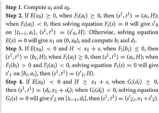
Algorithm 1. Search for the optimal solution of π_i1(S_i, t_i) under S_i < M + t_i−1.

Sales cycle greater than the trade credit, namely, s_i − t_i−1 ≥ M

Now, the retailer's profit function is π_i2(s, t). Taking the derivative of π_i2(s, t) with respect to t will give

$\begin{array}{ll}\frac{\partial {\pi }_{i2}(s,t)}{\partial t}={(\delta +\lambda )}^{-2}D(t)E(s,t).& (8)\end{array}$

where E(s, t) and E(x) are Equations 2, 3, respectively.

Lemma 5: For any given s and x₀ given by Equation 5, let t² is the maximum of π_i2(s, t) on [s, H]. Then, we will obtain the following conclusions:

(i) If E(x₀) ≥ 0 or E(x₀) < 0 and H < x₁ + s, then t² = H.

(ii) If E(x₀) < 0 and H ≥ x₁ + s, then $t^2=x_1+s$, where x₀ is computed by Equation 5, x₁is a unique solution of equation E(x) = 0 in the interval [0, x₀].

Proof. Similar to Lemma 1.

Lemma 5 reveals that t² is a function about s. Motivated by t = t²(s), we obtain ${\pi }_{i2}(s,t^2(s))$. Next, we search s ∈ [M + t_i−1, H] to let ${\pi }_{i2}(s,t^2(s))$ to obtain the maximum. According to Lemma 5, three cases are discussed as follows:

(a) E(x₀) ≥ 0. Now, t²(s) = H, taking the derivative of ${\pi }_{i2}(s,t^2(s))$ will give

$\begin{array}{ll}\frac{d{\pi }_{i2}(s,t^2(s))}{ds}=D(s)U_i(s)& (9)\end{array}$

where

$\begin{array}{l}{U}_i(s)=(p-c_0+c_2)[1-e^{-\delta (H-s)}]\\ -(c_0+h{\theta }^{-1})(e^{\theta (s-t_{i-1})}-1)+c_1(H-s)e^{-\delta (H-s)}\\ -c_0{I}_c{\theta }^{-1}(e^{\theta (s-M-t_{i-1})}-1)& (10)\end{array}$

Given that M + t_i−1 ≤ s ≤ t ≤ H and t²(s) = H, then M + t_i−1 ≤ s ≤ H. We summarize our finding for ${\pi }_{i2}(s,t^2(s))$ in Lemma 6.

Lemma 6: Let s² be the maximum point of ${\pi }_{i2}(s,t^2(s))$ on [M + t_i−1, H]. Then, the following conclusions are obtained:

(i) If U_i(M + t_i−1) ≤ 0, then $s^2=M+t_{i-1}$.

(ii) If U_i(H) ≥ 0, then s² = H.

(iii) If U_i(M + t_i−1) > 0 and U_i(H) < 0, then $s^2={s^{\prime }}_3$, where ${s^{\prime }}_3$ is a unique solution for U_i(s) = 0 in the interval [M + t_i−1, H].

Proof. Taking the derivative of U_i(s) will give

$\begin{array}{l}{U^{\prime }}_i(s)=-\delta (p-c_0+c_2)e^{-\delta (H-s)}-(\theta c_0+h)e^{\theta (s-t_{i-1})}\\ -c_1\left[1+\delta (H-s)\right]e^{-\delta (H-s)}-c_0{I}_c{e}^{\theta (s-M-t_{i-1})}.\end{array}$

Then, ${U^{\prime }}_i(s)<0$. Hence U_i(s) is a decreasing function about s.

If U_i(M + t_i−1) ≤ 0, based on ${U^{\prime }}_i(s)<0$, then U_i(s) ≤ 0, s ∈ [M + t_i−1, H], based on Equation 9, $d{\pi }_{i2}(s,t^2(s))/ds\le 0$, hence $s^2=M+t_{i-1}$.

If U_i(H) ≥ 0, based on ${U^{\prime }}_i(s)<0$, then U_i(s) ≥ 0, s ∈ [M + t_i−1, H]. Based on Equation 9, if s ∈ [M + t_i−1, H], then $d{\pi }_{i2}(s,t^2(s))/ds\le 0$, hence $s^2=M+t_{i-1}$.

If U_i(M + t_i−1) > 0 and U_i(H) < 0, based on the intermediate value theorem, equation U_i(s) = 0 holds a unique solution (denoted by ${s^{\prime }}_3$) in the interval (M + t_i−1, H), and only if $s\in (M+t_{i-1},{s^{\prime }}_3)$, U_i(s) > 0, if $s\in ({s^{\prime }}_3,H)$, U_i(s) < 0. From Equation 9, we get that if $s\in (M+t_{i-1},{s^{\prime }}_3)$, $d{\pi }_{i2}(s,t^2(s))/ds>0$; if $s\in ({s^{\prime }}_3,H)$, $d{\pi }_{i2}(s,t^2(s))/ds<0$, hence $s^2={s^{\prime }}_3$.

(b) E(x₀) < 0 and H < x₁ + s. Now, t²(s) = H. Given that s ≥ M + t_i−1, then k_i ≤ s ≤ H, where k_i = max{M + t_i−1, H − x₁}. We summarize our finding for ${\pi }_{i2}(s,t^2(s))$ in Lemma 7.

Lemma 7: Let s² be the maximum point of ${\pi }_{i2}(s,t^2(s))$ on [k_i, H]. Then, the following conclusions are obtained:

(i) If U_i(k_i) ≤ 0, then $s^2=k_i$.

(ii) If U_i(H) ≥ 0, then s² = H.

(iii) If U_i(k_i) > 0 and U_i(H) < 0, then $s^2={s^{\prime }}_4$, where ${s^{\prime }}_4$ is a unique solution for U_i(s) = 0 in the interval (k_i, H).

Proof. Given that U_i(s) is a decreasing function, three cases are discussed as follows:

If U_i(k_i) ≤ 0, from ${U^{\prime }}_i(s)<0$, then U_i(s) ≤ 0, s ∈ [k_i, H]. Based on Equation 9, when s ∈ [k_i, H], then $d{\pi }_{i2}(s,t^2(s))/ds\le 0$, hence ${\pi }_{i2}(s,t^2(s))$ is a decreasing function and $s^2=k_i$.

If U_i(H) ≥ 0, from ${U^{\prime }}_i(s)<0$, U_i(s) ≥ 0, s ∈ [k_i, H]. Based on Equation 9, when s ∈ [k_i, H], then $d{\pi }_{i2}(s,t^2(s))/ds\ge 0$ hence ${\pi }_{i2}(s,t^2(s))$ is an increasing function and s² = H.

If U_i(k_i) > 0 and U_i(H) < 0, based on the intermediate value theorem, U_i(s) = 0 holds a unique solution (denoted by ${s^{\prime }}_4$), and if $s\in (k_i,{s^{\prime }}_4)$, U_i(s) > 0; if $s\in ({s^{\prime }}_4,H)$, U_i(s) < 0. Based on Equation 9, if $s\in (k_i,s_4^{\prime })$, then $d{\pi }_{i2}(s,t^2(s))/ds>0$; if $s\in ({s^{\prime }}_4,H)$ then $d{\pi }_{i2}(s,t^2(s))/ds<0$, hence $s^2={s^{\prime }}_4$.

(c) E(x₀) < 0 and H ≥ x₁ + s. Now, $t^2(s)=x_1+s$, taking the derivative of ${\pi }_{i2}(s,t^2(s))$ will give

$\begin{array}{ll}\frac{d{\pi }_{i2}(s,t^2(s))}{ds}=D(s)V_i(s).& (11)\end{array}$

where

$\begin{array}{l}{V}_i(s)=(p-c_0+c_2)[1-e^{-\delta x_1}]-(c_0+h{\theta }^{-1})(e^{\theta (s-t_{i-1})}-1)\\ +c_1{x}_1{e}^{-\delta x_1}-c_0{I}_c{\theta }^{-1}(e^{\theta (s-M-t_{i-1})}-1).\end{array}$

Given that s ≥ M + t_i−1, t = x₁ + s, and t ≤ H, then M + t_i−1 ≤ s ≤ H − x₁. We summarize our finding for ${\pi }_{i2}(s,t^2(s))$ in Lemma 8.

Lemma 8: Let s² be the maximum point of ${\pi }_{i2}(s,t^2(s))$ on [M + t_i−1, H − x₁]. Then, the following conclusions are obtained:

(i) If V_i(M + t_i−1) ≤ 0, then $s^2=M+t_{i-1}$.

(ii) If V_i(H − x₁) ≥ 0, then $s^2=H-x_1$.

(iii) If V_i(M + t_i−1) > 0 and V_i(H − x₁) < 0, then $s^2={s^{\prime }}_5$, where ${s^{\prime }}_5$ is a unique solution for V_i(s) = 0 in the interval (M + t_i−1, H − x₁).

Proof. Taking the derivative of V_i(s) will give

$V_i^{\prime }(s)=-(\theta c_0+h)e^{\theta (s-t_{i-1})})-c_0{I}_c{e}^{\theta (s-M-t_{i-1})}.$

Then, ${V^{\prime }}_i(s)<0$, hence V_i(s) is a decreasing function about s.

If V_i(M + t_i−1) ≤ 0, based on ${V^{\prime }}_i(s)<0$, V_i(s) ≤ 0, s ∈ [M + t_i−1, H − x₁]. Based on Equation 11, if s ∈ [M + t_i−1, H − x₁], $d{\pi }_{i2}(s,t^2(s))/ds\le 0$, then $s^2=M+t_{i-1}$.

If V_i(H − x₁) ≥ 0, based on ${V^{\prime }}_i(s)<0$, V_i(s) ≥ 0, s ∈ [M + t_i−1, H − x₁]. Based on Equation 11, if s ∈ [M + t_i−1, H − x₁], $d{\pi }_{i2}(s,t^2(s))/ds\ge 0$, then $s^2=H-x_1$.

If V_i(M + t_i−1) > 0 and V_i(H − x₁) < 0, based on the intermediate value theorem, V_i(s) = 0 holds on a unique solution (denoted by ${s^{\prime }}_5$) in the interval (M + t_i−1, H − x₁), and only if $s\in (M+t_{i-1},{s^{\prime }}_5)$, V_i(s) > 0, if $s\in ({s^{\prime }}_5,H-x_1)$, V_i(s) < 0. From Equation 11, we learn that if $s\in (M+t_{i-1},{s^{\prime }}_5)$, $d{\pi }_{i2}(s,t^2(s))/ds>0$; if $s\in (s_5^{\prime },H-x_1)$, then $d{\pi }_{i2}(s,t^2(s))/ds<0$, hence $s^2={s^{\prime }}_5$.

Theorem 2. Let (s², t²) be the maximum of π_i2(s, t) such that it satisfies $s^1-t_{i-1}\ge M$ and $t_{i-1}\le s^1\le t^1\le H$. Then, the following conclusions are obtained:

(i) When E(x₀) ≥ 0, then t² = H, and if U_i(M + t_i−1) ≤ 0, $s^2=M+t_{i-1}$; if U_i(H) > 0, then s² = H; if U_i(M + t_i−1) > 0 and U_i(H) ≤ 0, then $s^2={s^{\prime }}_3$, where ${s^{\prime }}_3$ is a unique solution for U_i(s) = 0 in the interval [M + t_i−1, H].

(ii) When E(x₀) < 0 and H < x₁ + s, then t² = H, and if U_i(k_i) ≤ 0, then $s^2=k_i$; if U_i(H) ≥ 0, then s² = H; if U_i(k_i) > 0 and U_i(H) < 0, then $s^2={s^{\prime }}_4$, where ${s^{\prime }}_4$ is a unique solution for U_i(s) = 0 in the interval (k_i, H).

(iii) When E(x₀) < 0 and H ≥ x₁ + s, if V_i(M + t_i−1) ≤ 0, then $s^2=M+t_{i-1}$; if V_i(H − x₁) ≥ 0, then $s^2=H-x_1$; if V_i(M + t_i−1) > 0, and V_i(H − x₁) < 0, then $s^2={s^{\prime }}_5$, hence $t^2=x_1+s^2$, where ${s^{\prime }}_5$ is a unique solution for V_i(s) = 0 in the interval (M + t_i−1, H − x₁).

Based on Theorem 2, we can design Algorithm 2.

ALGORITHM 2

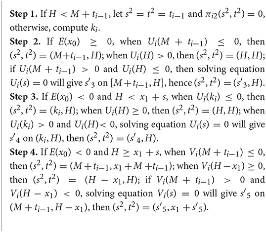
Algorithm 2. Search for the optimal solution of π_i2(S_i, t_i) under S_i ≥ M + t_i−1.

ALGORITHM 3

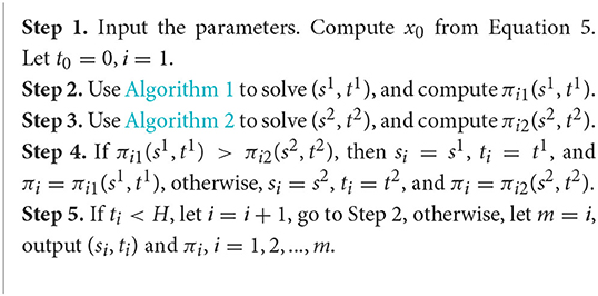
Algorithm 3. Solution for problem (P).

Numerical example

Example 1: The parameters of the inventory system, refer to Experiment 1 of Gupta et al.'s [47] model, are as follows: D₀ = 100, λ = 0.7, p = $2/unit, c₀ = $1/unit, c₁ = $0.8/unit, c₂ = $2/unit, h = $0.5/unit/month, I_e = 0.12/$/unit/month, I_c = 0.15/$/unit/month, θ = 0.08, δ = 0.9, M = 0.25 month, and H = 6 month. Using the proposed algorithm, we have two order strategies in Table 2 with different demand function.

TABLE 2

Table 2. Order strategies for example 1.

Table 2 shows the ordering strategies under two different demand functions, the finite horizon is divided into four sale cycles. Among them, the first three cycles are the same. Due to horizon limitation, the remaining time of the horizon is regarded as the fourth period. The total profit of the ordering policy with an increasing demand function is $4,437.2, which is smaller than that with a decreasing demand function ($5,113.9). The reason is that when the last cycle is insufficient, and demand is small, the impact on total profit is small and vice versa. The order quantity of the first three periods under the two ordering strategies has the change trend similar to the demand function.

Based on the initial value of system parameters from Example 1, the demand function is $D(t)=D_0{e}^{\lambda t}$. The effect of the main parameters (p, c₀, M, and θ) on total profit is shown in Figure 2.

FIGURE 2

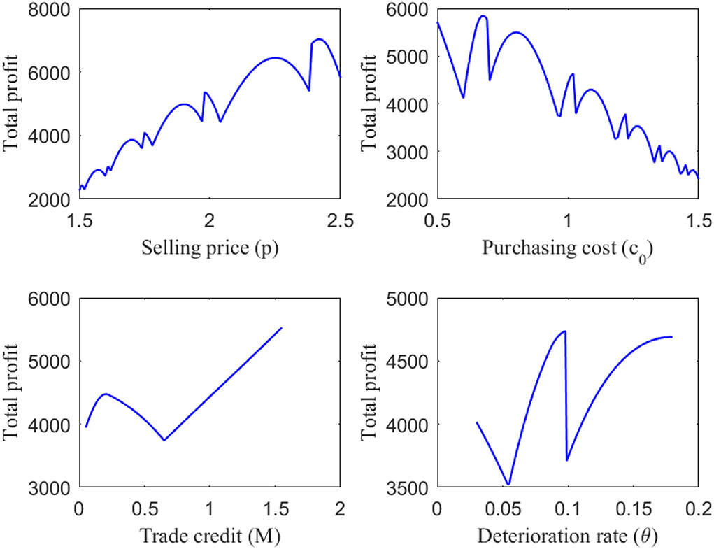
Figure 2. Effects of p, c₀, M, and θ on total profit.

Figure 2 reveals that total profit is increasing as the selling price increases in the interval (1.5, 2.5); the overall tendency of total profit is rising in the same way as the selling price in the interval. The figure of changes in total profit floats up and down irregularly, the reason is that the length of the last cycle depends on the finite horizon surplus under the first (m−1) equal cycles. Purchasing cost is outlay items, thus the overall tendency falls in the interval (0.5, 1.5), as mentioned above.

The effect on trade credit and the deterioration rate on total profit is drawn in the interval (Figure 2). The overall change trend of total profit with respect to these two parameters is increasing, but the range of change is larger because the sensitivity of these two parameters is higher. We analyzed the effects of selling price and purchase cost on total profit from a macro perspective. As for why the overall trend fluctuates, we can understand from a micro perspective by showing the important nodes of trade credit change.

To understand the reasons why the parameters affect total profit fluctuation in more detail, trade credit is taken as an example. Based on the parameters of Example 1 and the figures of several important nodes in trade credit, the total profit change data are studied in Table 3.

TABLE 3

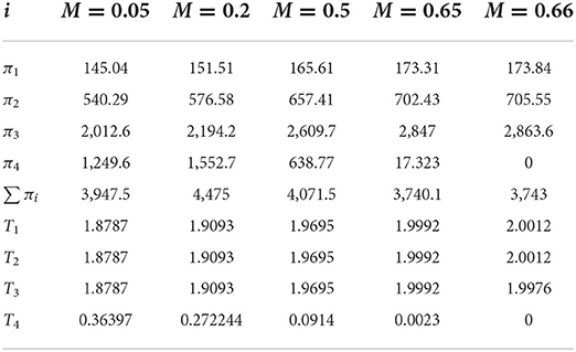
Table 3. Order strategies for different values of M.

Generally, total profit also rises with a rise in trade credit, details of the curve floating up or down are presented in Table 3. The first three cycles become longer as trade credit increases. However, the last cycle diminishes until it reaches 0, when M = 0.66, that is to say, there are only three cycles in finite horizon.

When M ∈ [0.05, 0.2] is increasing, the total profit increased from the first three cycles is greater than the decreased profit from the last one, hence the total profit is increasing. When M ∈ [0.2, 0.65] is increasing, the total profit increased from the first three cycles is less than the decreased profit from the last one, hence the total profit is decreasing. When M ∈ [0.66, 1.55] is increasing, order strategies only have three cycles, and the third cycle is basically the same as the first two cycles, that is, all three cycles are in the best sales state. As there is no limited planning period, this results in a very short cycle.

Conclusion

In this paper, a model for deteriorating products with multiple orders and partial backlogging under the condition of permissible delay in payments is studied. Suppose the deterioration rate of products is constant, the demand rate is a time-varying function, the backlogging rate is variable and dependent on the customer's waiting time for the next replenishment. Two kinds of situations for the model objective function are discussed, the existence and uniqueness of the optimal solution for each cycle are proven, a search algorithm corresponding to the order strategy is designed, and the optimality of each search step is presented. Ultimately, numerical examples are presented and the effect of the main parameters on total profit is analyzed.

Through the research conclusions of this paper, we can obtain some management enlightenment, listed as follows:

(1) By comparing the two demand functions, replenishment should be ensured as much as possible in the stage of a large demand during the finite horizon, so as to maximize retailers' overall profit.

(2) Sales price determination is also a very important consideration during the planning period as it affects not only the length and number of cycles, but also retailers' overall profit.

(3) As for trade credit and deterioration, through microscopic analysis, small changes in the parameters will lead to large changes in total profit, the reason of this factor is included in this paper.

At the same time, there are many shortcomings in this paper, which needs to be studied in the future. As for the partial backlogging rate, we only consider the waiting time of customers, and should also consider the price discount and other issues. In addition, global warming and carbon emissions are also significant factors for inventories and supply chains. I hope to be able to study a more realistic inventory model.

Data availability statement

The original contributions presented in the study are included in the article/supplementary material, further inquiries can be directed to the corresponding author.

Author contributions

Conceptualization: ZL and JM. Investigation: ZL, PC, and LN. Methodology and validation: ZL, JM, and PC. Writing—original draft preparation: ZL. Writing—review and editing: PC and LN. All authors contributed to the article and approved the submitted version.

Funding

This project was funded by the Natural Science Foundation of Guangxi Province (2020GXNSFAA297010 and 2021GXNSFBA220033) and Middle-aged and Young Teachers' Basic Ability Promotion Project of Guangxi (2021KY1563 and 2021KY0651). This work was also supported by Guangxi First-class Discipline Statistics Construction Project Fund (SXYB12).

Acknowledgments

The authors would like to thank the editors and reviewers for their valuable and constructive comments, which have led to a significant improvement in the manuscript.

Conflict of interest

The authors declare that the research was conducted in the absence of any commercial or financial relationships that could be construed as a potential conflict of interest.

Publisher's note

All claims expressed in this article are solely those of the authors and do not necessarily represent those of their affiliated organizations, or those of the publisher, the editors and the reviewers. Any product that may be evaluated in this article, or claim that may be made by its manufacturer, is not guaranteed or endorsed by the publisher.

References

1. Huang C, Cao J. Comparative study on bifurcation control methods in a fractional-order delayed predator-prey system. Sci China Technol Sci. (2019) 62:298–307. doi: 10.1007/s11431-017-9196-4

CrossRef Full Text | Google Scholar

2. Liu H, Wang H, Cao J, Alsaedi A, Hayat T. Composite learning adaptive sliding mode control of fractional-order nonlinear systems with actuator faults. J Franklin Inst. (2019) 356:9580–99. doi: 10.1016/j.jfranklin.2019.02.042

CrossRef Full Text | Google Scholar

3. Xue G, Lin F, Li S, Liu H. Adaptive dynamic surface control for finite-time tracking of uncertain nonlinear systems with dead-zone inputs and actuator faults. Int J Control Autom Syst. (2021) 19:2797–811. doi: 10.1007/s12555-020-0441-6

CrossRef Full Text | Google Scholar

4. Liu H, Pan Y, Cao J, Zhou Y, Wang H. Positivity and stability analysis for fractional-order delayed systems: a T-S fuzzy model approach. IEEE Trans Fuzzy Syst. (2021) 29:927–39. doi: 10.1109/TFUZZ.2020.2966420

CrossRef Full Text | Google Scholar

5. Xue G, Lin F, Li S, Liu H. Adaptive fuzzy finite-time backstepping control of fractional-order nonlinear systems with actuator faults via command-filtering and sliding mode technique. Inf Sci. (2022) 600:189–208. doi: 10.1016/j.ins.2022.03.084

CrossRef Full Text | Google Scholar

6. Goyal SK, Morin D, Nebebe F. The finite horizon trended inventory replenishment problem with shortages. J Oper Res Soc. (2017) 43:1173–8. doi: 10.1057/jors.1992.183

CrossRef Full Text | Google Scholar

7. Kar S, Bhunia AK, Maiti M. Deterministic inventory model with two levels of storage, a linear trend in demand and a fixed time horizon. Comput Oper Res. (2001) 28:1315–31. doi: 10.1016/S0305-0548(00)00042-3

CrossRef Full Text | Google Scholar

8. Sana SS. Optimal selling price and lotsize with time varying deterioration and partial backlogging. Appl Math Comput. (2010) 217:185–94. doi: 10.1016/j.amc.2010.05.040

CrossRef Full Text | Google Scholar

9. Yung-Fu H. Economic order quantity under conditionally permissible delay in payments. Eur J Oper Res. (2007) 176:911–24. doi: 10.1016/j.ejor.2005.08.017

CrossRef Full Text | Google Scholar

10. Dye C. A finite horizon deteriorating inventory model with two-phase pricing and time-varying demand and cost under trade credit financing using particle swarm optimization. Swarm Evol Comput. (2012) 5:37–53. doi: 10.1016/j.swevo.2012.03.002

CrossRef Full Text | Google Scholar

11. Goyal SK. Economic order quantity under conditions of permissible delay in payment. J Oper Res Soc. (1985) 36:335–8. doi: 10.1057/jors.1985.56

CrossRef Full Text | Google Scholar

12. Ouyang L, Teng J, Goyal SK, Yang C. An economic order quantity model for deteriorating items with partially permissible delay in payments linked to order quantity. Eur J Oper Res. (2009) 194:418–31. doi: 10.1016/j.ejor.2007.12.018

CrossRef Full Text | Google Scholar

13. Chung K, Goyal SK, Huang Y. The optimal inventory policies under permissible delay in payments depending on the ordering quantity. Int J Prod Econ. (2005) 95:203–13. doi: 10.1016/j.ijpe.2003.12.006

CrossRef Full Text | Google Scholar

14. Chung K, Liao J. Lot-sizing decisions under trade credit depending on the ordering quantity. Comput Oper Res. (2004) 31:909–28. doi: 10.1016/S0305-0548(03)00043-1

CrossRef Full Text | Google Scholar

15. Chung K, Liao J. The optimal ordering policy in a DCF analysis for deteriorating items when trade credit depends on the order quantity. Int J Prod Econ. (2006) 100:116–30. doi: 10.1016/j.ijpe.2004.10.011

CrossRef Full Text | Google Scholar

16. Kreng VB, Tan S. The optimal replenishment decisions under two levels of trade credit policy depending on the order quantity. Expert Syst Appl. (2010) 37:5514–22. doi: 10.1016/j.eswa.2009.12.014

CrossRef Full Text | Google Scholar

17. Ouyang L, Ho C, Su C. An optimization approach for joint pricing and ordering problem in an integrated inventory system with order-size dependent trade credit. Comput Ind Eng. (2009) 57:920–30. doi: 10.1016/j.cie.2009.03.011

CrossRef Full Text | Google Scholar

18. Yu JCP. Optimizing a two-warehouse system under shortage backordering, trade credit, and decreasing rental conditions. Int J Prod Econ. (2019) 209:147–55. doi: 10.1016/j.ijpe.2018.06.003

CrossRef Full Text | Google Scholar

19. Chen S, Cárdenas-Barrón LE, Teng J. Retailer's economic order quantity when the supplier offers conditionally permissible delay in payments link to order quantity. Int J Prod Econ. (2014) 155:284–91. doi: 10.1016/j.ijpe.2013.05.032

CrossRef Full Text | Google Scholar

20. Tiwari S, Cárdenas-Barrón LE, Shaikh AA, Goh M. Retailer's optimal ordering policy for deteriorating items under order-size dependent trade credit and complete backlogging. Comput Ind Eng. (2020) 139:105559. doi: 10.1016/j.cie.2018.12.006

CrossRef Full Text | Google Scholar

21. Xu C, Zhao D, Min J, Hao J. An inventory model for nonperishable items with warehouse mode selection and partial backlogging under trapezoidal-type demand. J Oper Res Soc. (2021) 72:744–63. doi: 10.1080/01605682.2019.1708822

CrossRef Full Text | Google Scholar

22. Chang C, Teng J, Chern M. Optimal manufacturer's replenishment policies for deteriorating items in a supply chain with up-stream and down-stream trade credits. Int J Prod Econ. (2010) 127:197–202. doi: 10.1016/j.ijpe.2010.05.014

CrossRef Full Text | Google Scholar

23. Tiwari S, Cárdenas-Barrón LE, Goh M, Shaikh AA. Joint pricing and inventory model for deteriorating items with expiration dates and partial backlogging under two-level partial trade credits in supply chain. Int J Prod Econ. (2018) 200:16–36. doi: 10.1016/j.ijpe.2018.03.006

CrossRef Full Text | Google Scholar

24. Vandana, Kaur, A. Two-level trade credit with default risk in the supply chain under stochastic demand. Omega. (2019) 88:4–23. doi: 10.1016/j.omega.2018.12.003

CrossRef Full Text | Google Scholar

25. Zou X, Tian B. Retailer's optimal ordering and payment strategy under two-level and flexible two-part trade credit policy. Comput Ind Eng. (2020) 142:106317. doi: 10.1016/j.cie.2020.106317

CrossRef Full Text | Google Scholar

26. Panda S, Senapati S, Basu M. Optimal replenishment policy for perishable seasonal products in a season with ramp-type time dependent demand. Comput Ind Eng. (2008) 54:301–14. doi: 10.1016/j.cie.2007.07.011

CrossRef Full Text | Google Scholar

27. Dey JK, Mondal SK, Maiti M. Two storage inventory problem with dynamic demand and interval valued lead-time over finite time horizon under inflation and time-value of money. Eur J Oper Res. (2008) 185:170–94. doi: 10.1016/j.ejor.2006.12.037

CrossRef Full Text | Google Scholar

28. Lin J, Chao HCJ, Julian P. Planning horizon for production inventory models with production rate dependent on demand and inventory level. J Appl Math. (2013) 2013:1–9. doi: 10.1155/2013/961258

CrossRef Full Text | Google Scholar

29. Palanivel M, Priyan S, Mala P. Two-warehouse system for non-instantaneous deterioration products with promotional effort and inflation over a finite time horizon. J Ind Eng Int. (2018) 14:603–12. doi: 10.1007/s40092-017-0250-6

CrossRef Full Text | Google Scholar

30. Udayakumar R, Geetha KV. Economic ordering policy for single item inventory model over finite time horizon. Int J Syst Assur Eng Manag. (2017) 8:734–57. doi: 10.1007/s13198-016-0516-1

CrossRef Full Text | Google Scholar

31. Pramanik P, Maiti MK. An inventory model for deteriorating items with inflation induced variable demand under two level partial trade credit: a hybrid ABC-GA approach. Eng Appl Artif Intell. (2019) 85:194–207. doi: 10.1016/j.engappai.2019.06.013

CrossRef Full Text | Google Scholar

32. Xu C, Wang C, Ren J, Kang L, Du D. Online-retail supply chain optimization with credit period and selling price-dependent demand. Asia Pac J Oper Res. (2021) 2240004.

Google Scholar

33. Jaggi CK, Yadavalli VSS, Verma M, Sharma A. An EOQ model with allowable shortage under trade credit in different scenario. Appl Math Comput. (2015) 252:541–51. doi: 10.1016/j.amc.2014.12.040

CrossRef Full Text | Google Scholar

34. Hui-Ling Y. Two-warehouse inventory models for deteriorating items with shortages under inflation. Eur J Oper Res. (2004) 157:344–56. doi: 10.1016/S0377-2217(03)00221-2

CrossRef Full Text | Google Scholar

35. Jaggi CK, Pareek S, Khanna A, Sharma R. Credit financing in a two-warehouse environment for deteriorating items with price-sensitive demand and fully backlogged shortages. Appl Math Model. (2014) 38:5315–33. doi: 10.1016/j.apm.2014.04.025

CrossRef Full Text | Google Scholar

36. San-José LA, Sicilia J, González-de-la-Rosa M, Febles-Acosta J. Optimal price and lot size for an EOQ model with full backordering under power price and time dependent demand. Mathematics. (2021) 9:1848. doi: 10.3390/math9161848

CrossRef Full Text | Google Scholar

37. Nath BK, Sen N. A completely backlogged two-warehouse inventory model for non-instantaneous deteriorating items with time and selling price dependent demand. Int J Appl Comput Math. (2021) 7:1–22. doi: 10.1007/s40819-021-01070-x

CrossRef Full Text | Google Scholar

38. Sicilia J, San-José LA, Alcaide-López-de-Pablo D, Abdul-Jalbar B. Optimal policy for multi-item systems with stochastic demands, backlogged shortages and limited storage capacity. Appl Math Modell. (2022) 108:236–57. doi: 10.1016/j.apm.2022.03.025

CrossRef Full Text | Google Scholar

39. Hui-Ling Y. Two-warehouse partial backlogging inventory models for deteriorating items under inflation. Int J Prod Econ. (2006) 103:362–70. doi: 10.1016/j.ijpe.2005.09.003

CrossRef Full Text | Google Scholar

40. Yang H, Chang C. A two-warehouse partial backlogging inventory model for deteriorating items with permissible delay in payment under inflation. Appl Math Model. (2013) 37:2717–26. doi: 10.1016/j.apm.2012.05.008

CrossRef Full Text | Google Scholar

41. Hsieh T, Dye C. Pricing and lot-sizing policies for deteriorating items with partial backlogging under inflation. Expert Syst Appl. (2010) 37:7234–42. doi: 10.1016/j.eswa.2010.04.004

CrossRef Full Text | Google Scholar

42. Khan MA, Shaikh AA, Panda GC, Bhunia AK, Konstantaras I. Non-instantaneous deterioration effect in ordering decisions for a two-warehouse inventory system under advance payment and backlogging. Ann Oper Res. (2020) 289:243–75. doi: 10.1007/s10479-020-03568-x

CrossRef Full Text | Google Scholar

43. Sumon S, Bibhas CG. Safety stock management in a supply chain model with waiting time and price discount dependent backlogging rate in stochastic environment. Oper Res. (2020) 22:1–30. doi: 10.1007/s12351-020-00587-1

CrossRef Full Text | Google Scholar

44. Soni HN, Suthar DN. Optimal pricing and replenishment policy for non-instantaneous deteriorating items with varying rate of demand and partial backlogging. OPSEARCH. (2020) 57:986–1021. doi: 10.1007/s12597-020-00451-y

CrossRef Full Text | Google Scholar

45. Rana RS, Kumar D, Prasad K. Two warehouse dispatching policies for perishable items with freshness efforts, inflationary conditions and partial backlogging. Oper Manag Res. (2021) 15:1–18. doi: 10.1007/s12063-020-00168-7

CrossRef Full Text | Google Scholar

46. Palanivel M, Uthayakumar R. Finite horizon EOQ model for non-instantaneous deteriorating items with price and advertisement dependent demand and partial backlogging under inflation. Int J Syst Sci. (2015) 46:1762–73. doi: 10.1080/00207721.2013.835001

CrossRef Full Text | Google Scholar

47. Gupta M, Tiwari S, Jaggi CK. Retailer's ordering policies for time-varying deteriorating items with partial backlogging and permissible delay in payments in a two-warehouse environment. Ann Oper Res. (2020) 295:139–61. doi: 10.1007/s10479-020-03673-x

CrossRef Full Text | Google Scholar