Global Dynamics of a Delayed Fractional-Order Viral Infection Model With Latently Infected Cells

In this paper, we propose a fractional-order viral infection model, which includes latent infection, a Holling type II response function, and a time-delay representing viral production. Based on the characteristic equations for the model, certain sufficient conditions guarantee local asymptotic stability of infection-free and interior steady states. Whenever the time-delay crosses its critical value (threshold parameter), a Hopf bifurcation occurs. Furthermore, we use LaSalle’s invariance principle and Lyapunov functions to examine global stability for infection-free and interior steady states. Our results are illustrated by numerical simulations.

1 Introduction

Various mathematical models have been developed to describe, within-host, the dynamics of various viral infections, with a focus on virus-to-cell transmission, such as human immunodeficiency virus (HIV) [1], COVID-19 [2,3], hepatitis C virus (HCV) [4], hepatitis B virus (HBV) [5], and human T-cell lymphotropic virus 1 (HTLV-1) [6]. Classical viral infection models are composed of the interactions between susceptible cells, infected target cells, and free viruses. Furthermore, some authors studied latent infection to describe the mechanism of latency. Wang et al. [7] investigated the HIV model with latent infection incorporating both modes of time-delays and transmissions between viral entry and viral production or integration and also discussed the basic reproductive number, showing existence of asymptotic stability of endemic equilibrium points. Wen et al. [8] studied the virus-to-cell and cell-to-cell HIV virus transmission dynamics with latently infected cells. Pan et al. [9] discussed the HCV infection model, which includes the routes of infection and spread, such as virus-to-cell and cell-to-cell transmission dynamics, and explained numerically the four different HCV models.

The infection persists when the virus weakens and suppresses the immune response. Immune system response refers to the process that when the virus enters the human body, the immune system receives the signal of virus attack and spreads it to the immune organs, which secrete lymphocytes to purge the virus. Moreover, the adaptive immune response plays a crucial role in the control of infection process. When the virus spreads in the human body, the human body produces double modes of immune responses: one is the B cell that makes humoral immune response and the other is the cytotoxic T lymphocyte (CTL) that makes cellular immune response. Previous studies have shown that the humoral immune response is more active than the cellular immune responses. Elaiw et al. [10] discussed the dynamical behaviors of viral infection models with latently infected cells, humoral immune response, and general non-linear incidence rate function. The authors in [11] investigated the global asymptotic stability of reaction–diffusion viral infection model with homogeneous environments and non-linear incidence in heterogeneous and humoral immunity. Wang et al. [12] discussed the global stability results of HIV viral infection model with latently infected cells, B-cell immune response, Beddington–DeAngelis functional response, and various time-delays. The authors in [13] reported the stability and bifurcation results of generalized viral infection system with humoral immunity and distributed delays in virus production and cell infection, and time lags described the time needed to activate the immune response.

The fractional-order modeling provides more reliable, accurate, and precise information about the dynamics of biological models. Description of memory and hereditary properties make it superior to the classical-order model. Additionally, non-integer–order models can easily demonstrate and explore the dynamics between two non-local points and are more comprehensive to discuss real-world problems for the global dynamics. In recent years, various ideas and theories about the fractional-order derivatives have been developed and introduced (see [14–16]). Rakkiyappan et al. [17] discussed the fractional-order Zika viral infection model with different time-delays, such as the latency infection in the infected host and in a vector, and sufficient conditions for stability and bifurcation results with respect to time lags. The authors in [18] analyzed the local stability results of fractional-order Ebola viral infection model with time-delayed immune response (cytotoxic T-lymphocyte term) in heterogeneous complex networks. Rihan et al. [19] studied the fractional-order dynamics of hepatitis C virus (HCV) incorporating the intracellular delay between the initial infection of a cell by HCV and the release of new virions and the interferon-α (IFN-α) treatment. Tamilalagan et al. [20] reported the characteristic dynamics for the non-integer–order HIV infection model with CTL immune responses and antibody and also compared it with that of the integer-order model. The authors reported in [21] derived the sufficient conditions of stability and optimal control results for the fractional-order HIV model with transmission dynamics. Researchers investigated fractional-order viral infection models to understand how the immune system works and examined how immune cells eliminate virus [22,23].

With motivation of the above-mentioned studies, in this paper, we extend the integer-order differential model into the fractional-order model for the virus-immune system with latently infected cell compartments. We incorporate fractional order and time-delay to represent long-run and short-run memory. As part of the Holling type II functional response, viral pathogens spread from virus to cell and from cell to cell. To avoid dimensional mismatches in the fractional equations, a parameter modification is used. We derive the positivity and boundedness of the solution for the considered model. We examine the local stability of existing equilibrium points and the bifurcation results of the considered model. We also discuss some necessary conditions for global stability using a novel suitable Lyapunov function combined with LaSalle’s invariance principle. The rest of this paper is organized as follows: In Section 2, we formulate the viral infection model and also study the positivity and boundedness of the solution. Local and global stability results of such a model are derived in Section 3 and Section 4, respectively. The numerical simulations are provided in Section 5, to validate the obtained theoretical results. Section 6 contains conclusion.

2 Model Formulation

In the process of viral infection, the immune system plays a critical role. Viral dynamics can be modeled properly to provide insights into understanding the disease and the clinical treatments used to treat it. In adaptive immune responses, lymphocytes are responsible for specificity and memory. The two main types of lymphocytes are B cells and T cells. The function of T cells is to recognize and kill infected cells, while the function of B cells is to produce antibodies to neutralize the viruses. Researchers have studied the effects of immune responses such as CTL responses and antibody responses [24–27]. Some other researchers have also taken into account the effect of CTL responses and intracellular delays [16,19,28]. The mathematical model that describes the effect of humoral immune response on virus dynamics is presented as [29]

$\begin{array}{cc}\hfill \dot{x}\left(t\right)& =\widehat{\lambda }-\widehat{d}x\left(t\right)-\widehat{{\beta }_1}x\left(t\right)v\left(t\right)-\widehat{{\beta }_2}x\left(t\right)y\left(t\right),\hfill \\ \hfill \dot{y}\left(t\right)& =\widehat{{\beta }_1}x\left(t\right)v\left(t\right)+\widehat{{\beta }_2}x\left(t\right)y\left(t\right)-\widehat{a}y\left(t\right),\hfill \\ \hfill \dot{v}\left(t\right)& =\widehat{k}y\left(t\right)-\widehat{\mu }v\left(t\right)-\widehat{\xi }v\left(t\right)w\left(t\right),\hfill \\ \hfill \dot{w}\left(t\right)& =\widehat{g}v\left(t\right)w\left(t\right)-\widehat{h}w\left(t\right),\hfill \end{array}(1)$

where x(t), y(t), v(t), and w(t) represent the concentration of uninfected target cells, actively infected cells, free viruses, and antibodies/B cells at time t, respectively. The uninfected cells x(t) are assumed to produce/grow at a constant rate $\widehat{\lambda }$ and death rate $\widehat{d}$. $\widehat{{\beta }_1}$ is the infection rate by free virus, and $\widehat{{\beta }_2}$ is the rate at which uninfected cells are converted to productively infected ones per both cells. $\widehat{a},\widehat{\mu },\widehat{h}$ are the death rate of infected cells, free virus particles, and antibodies/B cells, respectively. Free virus particles are produced from productively infected cells at the rate $\widehat{k}$, and $\widehat{\xi }$ is the rate of neutralization by antibodies. $\widehat{g}$ is the rate of antibodies activated against the virus.

Herein, we upgrade the model (1) to include the latent infection component. We assume that the uninfected cell x(t) becomes infected by free virus or by direct contact with an infected cell at the rate $\frac{\widehat{{\beta }_1}x(t)v(t)}{1+v(t)}+\frac{\widehat{{\beta }_2}x(t)y(t)}{1+y(t)}$ with Holling type II functional response. We also assume that (1 − φ) and φ ∈ (0, 1) are the proportions of infection that lead to latency and productivity, respectively. A fractional order (0 < α ≤ 1) is also considered in the model to represent the long-run memory. The model takes the form

$\begin{array}{cc}\hfill D^{\alpha }x\left(t\right)& =\lambda -dx\left(t\right)-\frac{{\beta }_{1}x\left(t\right)v\left(t\right)}{1+v\left(t\right)}-\frac{{\beta }_{2}x\left(t\right)y\left(t\right)}{1+y\left(t\right)},\hfill \\ \hfill D^{\alpha }l\left(t\right)& =\left(1-\phi \right)\left(\frac{{\beta }_{1}x\left(t\right)v\left(t\right)}{1+v\left(t\right)}+\frac{{\beta }_{2}x\left(t\right)y\left(t\right)}{1+y\left(t\right)}\right)-\left(m+\gamma \right)l\left(t\right),\hfill \\ \hfill D^{\alpha }y\left(t\right)& =\phi \left(\frac{{\beta }_{1}x\left(t\right)v\left(t\right)}{1+v\left(t\right)}+\frac{{\beta }_{2}x\left(t\right)y\left(t\right)}{1+y\left(t\right)}\right)+\gamma l\left(t\right)-ay\left(t\right),\hfill \\ \hfill D^{\alpha }v\left(t\right)& =k{e}^{-m_1\tau }y\left(t-\tau \right)-\mu v\left(t\right)-\xi v\left(t\right)w\left(t\right),\hfill \\ \hfill D^{\alpha }w\left(t\right)& =gv\left(t\right)w\left(t\right)-hw\left(t\right),\hfill \end{array}(2)$

with initial values x(0) > 0, l(0) > 0, y(s) = χ(s) > 0, v(0) > 0, w(0) > 0, s ∈ [ − τ, 0] and χ(s) being the smooth function. Here, D^α is the Caputo fractional derivative of order α. l(t) denotes the concentrations of infected cells in the latent stage at t. We avoid dimensional mismatches for the fractional order model, define the parameter values $\lambda ={\widehat{\lambda }}^{\alpha },{\beta }_1={\widehat{{\beta }_1}}^{\alpha },{\beta }_2={\widehat{{\beta }_2}}^{\alpha },a={\widehat{a}}^{\alpha },k={\widehat{k}}^{\alpha },m_1={\widehat{m}}_1^{\alpha },\mu ={\widehat{\mu }}^{\alpha },\xi ={\widehat{\xi }}^{\alpha },g={\widehat{g}}^{\alpha },h={\widehat{h}}^{\alpha },$ and $m={\widehat{m}}^{\alpha }$ be the death rate of l(t) and latent infection become productively infected cells at the rate $\gamma ={\widehat{\gamma }}^{\alpha }$. τ is delay which defines the time it takes for the newly produced virus to be mature and then infectious. $e^{-m_1\tau }$ is the survival probability of immature virions.

Definition 1 [15]. The Caputo derivative of fractional order α for a function f(t) is described as

$D^{\alpha }f\left(t\right)=\frac{1}{\mathrm{\Gamma }\left(n-\alpha \right)}{\int }_0^t{\left(t-\tau \right)}^{n-\alpha -1}{f}^n\left(\tau \right)d\tau ,$

where $n-1<\alpha <n\in {\mathbb{Z}}^{+}$ and Γ(⋅) is the gamma function.

The Laplace transform of Caputo derivative is described as

$\mathcal{L}\left\{D^{\alpha }f\left(t\right);s\right\}=s^{\alpha }\mathcal{F}\left(s\right)-\sum _{i=1}^{n-1}{s}^{\alpha -i-1}{f}^{\left(i\right)}\left(0\right),$

where $\mathcal{F}(s)=\mathcal{L}\{f(t)\}$. In particular, when f⁽ⁱ⁾(0) = 0, i = 1, 2, …, n − 1, then $\mathcal{L}\{D^{\alpha }f(t);s\}=s^{\alpha }\mathcal{F}(s)$.

Remark 1. The fractional derivative α ∈ (0, 1) is defined by Caputo sense [15], so introducing a convolution integral with a power-law memory kernel is a good way to describe memory effects in dynamical systems. The decaying rate of the memory kernel is determined by α. A lower value of α corresponds to slower-decaying time-correlation functions which result in long-run memory.

Theorem 1. For any initial values x(0) > 0, l(0) > 0, y(s) = χ(s) > 0, v(0) > 0, w(0) > 0, s ∈ [ − τ, 0], the model (2) has a unique solution in [0, + ∞). Moreover, this solution remains positive and bounded.

Proof 1. Assume that ${\mathbb{R}}_{+}^5=\{(x,l,y,v,w)\in {\mathbb{R}}^5:x\ge 0,l\ge 0,y\ge 0v\ge 0,w\ge 0\}$ is positively invariant. The model (2) becomes

$D^{\alpha }Z\left(t\right)=\mathcal{K}\left(Z\left(t\right)\right).$

Here, Z(t) = (x(t),l(t),y(t),v(t),w(t))^T, and

$\mathcal{K}\left(Z\left(t\right)\right)=\left[\begin{array}{c}\hfill \lambda -dx\left(t\right)-\frac{{\beta }_{1}x\left(t\right)v\left(t\right)}{1+v\left(t\right)}-\frac{{\beta }_{2}x\left(t\right)y\left(t\right)}{1+y\left(t\right)}\hfill \\ \hfill \left(1-\phi \right)\left(\frac{{\beta }_{1}x\left(t\right)v\left(t\right)}{1+v\left(t\right)}+\frac{{\beta }_{2}x\left(t\right)y\left(t\right)}{1+y\left(t\right)}\right)-\left(m+\gamma \right)l\left(t\right)\hfill \\ \hfill \phi \left(\frac{{\beta }_{1}x\left(t\right)v\left(t\right)}{1+v\left(t\right)}+\frac{{\beta }_{2}x\left(t\right)y\left(t\right)}{1+y\left(t\right)}\right)+\gamma l\left(t\right)-ay\left(t\right)\hfill \\ \hfill k{e}^{-m_1\tau }y\left(t-\tau \right)-\mu v\left(t\right)-\xi v\left(t\right)w\left(t\right)\hfill \\ \hfill gv\left(t\right)w\left(t\right)-hw\left(t\right)\hfill \end{array}\right].$

$Z_0={(x(0),l(0),y(s),v(0),w(0))}^T\in {\mathbb{R}}_{+}^5$. For that, we analyze the direction of $\mathcal{K}(Z(t))$ on each coordinate space and see whether the vector field points to the interior of ${\mathbb{R}}_{+}^5$. From Eq. 2, we get

$\begin{array}{cc}\hfill D^{\alpha }x\left(t\right){|}_{x=0}& =\lambda \ge 0,\hfill \\ \hfill D^{\alpha }l\left(t\right){|}_{l=0}& =\left(1-\phi \right)\left(\frac{{\beta }_{1}x\left(t\right)v\left(t\right)}{1+v\left(t\right)}+\frac{{\beta }_{2}x\left(t\right)y\left(t\right)}{1+y\left(t\right)}\right)\ge 0,\hfill \\ \hfill D^{\alpha }y\left(t\right){|}_{y=0}& =\phi \frac{{\beta }_{1}x\left(t\right)v\left(t\right)}{1+v\left(t\right)}+\gamma l\left(t\right)\ge 0,\hfill \\ \hfill D^{\alpha }v\left(t\right){|}_{v=0}& =k{e}^{-m_1\tau }y\left(t-\tau \right)\ge 0,\hfill \\ \hfill D^{\alpha }w\left(t\right){|}_{w=0}& =0.\hfill \end{array}(3)$

From [30,31] and Eq. 3, we found $\mathcal{K}(Z(t))$ is interior of ${\mathbb{R}}_{+}^5$. The solution of Eq. 2 with $Z_0\in {\mathbb{R}}_{+}^5$ is Z(t) = Z(t, Z₀), in such a way that $Z(t)\in {\mathbb{R}}_{+}^5$.

Next, we prove the boundedness, adding the first three equations in Eq. 2:

$D^{\alpha }\left\{x\left(t\right)+l\left(t\right)+y\left(t\right)\right\}=\lambda -dx\left(t\right)-ml\left(t\right)-ay\left(t\right).$

Suppose that d ≤ min{m, a}, we get

$D^{\alpha }\left\{x\left(t\right)+l\left(t\right)+y\left(t\right)\right\}\le \lambda -d\left\{x\left(t\right)+l\left(t\right)+y\left(t\right)\right\}.$

If t → ∞, then we get $x(t)+l(t)+y(t)\le \frac{\lambda }{d}$. The fourth equation of Eq. 2 is

$D^{\alpha }v\left(t\right)\le k{e}^{-m_1\tau }\frac{\lambda }{d}-\mu v\left(t\right).$

If t → ∞, then we get $v(t)\le k{e}^{-m_1\tau }\frac{\lambda }{\mu d}$. We can easily prove the boundedness of w(t).

The model (2) has the following equilibrium points:

• Infection-free equilibrium point ${\mathcal{E}}_0(\frac{\lambda }{d},\mathrm{0,0,0,0})$.

• Immune response–free equilibrium point ${\mathcal{E}}_1(x*,l*,y*=\frac{\mu h}{kg},v*=\frac{h}{g},0)$ where $x*=\frac{\lambda }{d+\frac{{\beta }_{1}h}{g+h}+\frac{{\beta }_2\mu h}{kg+\mu h}}$, $l*=\frac{(1-\phi )\left(\frac{{\beta }_{1}x*v*}{1+v*}+\frac{{\beta }_{2}x*y*}{1+y*}\right)}{m+\gamma }$.

• Endemic equilibrium point ${\mathcal{E}}_2(x*,l*,y*,v*,w*)$ where $l*=\frac{(1-\phi )(\lambda -dx*)}{m+\gamma }$, $y*=\frac{(\gamma +\phi m)(\lambda -dx*)}{a(m+\gamma )},v*=\frac{h}{g}$, $w*=\frac{gk(\gamma +\phi m)(\lambda -dx*)-\mu ha(m+\gamma )}{a\xi h(m+\gamma )}$. Since l^*, y^*, w^* > 0, we must have $x*<\frac{\lambda }{d}$ and $x*\in (0,\frac{\lambda }{d})$ satisfy the following quadratic equation:

$\left(a\left(m+\gamma \right)+\left(\lambda -dx*\right)\left(\gamma +\phi m\right)\right)\left(\left(\lambda -dx*\right)\left(g+h\right)+{\beta }_{1}x*h\right)+{\beta }_{2}x*\left(\lambda -dx*\right)\left(\gamma +\phi m\right)\left(g+h\right)=0.$

Here, we derive the threshold quantity ${\mathcal{R}}_0$ and define the transmission matrix $\mathbb{F}$ and transition matrix $\mathbb{V}$ as follows:

$\mathbb{F}=\left[\begin{array}{cccc}\hfill 0\hfill & \hfill {\beta }_{2}x*\left(1-\phi \right)\hfill & \hfill {\beta }_{1}x*\left(1-\phi \right)\hfill & \hfill 0\hfill \\ \hfill 0\hfill & \hfill {\beta }_{2}x*\phi \hfill & \hfill {\beta }_{1}x*\phi \hfill & \hfill 0\hfill \\ \hfill 0\hfill & \hfill 0\hfill & \hfill 0\hfill & \hfill 0\hfill \\ \hfill 0\hfill & \hfill 0\hfill & \hfill 0\hfill & \hfill 0\hfill \end{array}\right]\text{and}\mathbb{V}=\left[\begin{array}{cccc}\hfill m+\gamma \hfill & \hfill 0\hfill & \hfill 0\hfill & \hfill 0\hfill \\ \hfill -\gamma \hfill & \hfill a\hfill & \hfill 0\hfill & \hfill 0\hfill \\ \hfill 0\hfill & \hfill -k{e}^{-m_1\tau }\hfill & \hfill \mu \hfill & \hfill 0\hfill \\ \hfill 0\hfill & \hfill 0\hfill & \hfill 0\hfill & \hfill h\hfill \end{array}\right].$

Based on the method of next-generation matrix [32–34], the threshold quantity ${\mathcal{R}}_0$ is the spectral radius of

${\mathbb{FV}}^{-1}=\left[\begin{array}{cccc}\hfill \frac{\gamma {\beta }_{2}x*\left(1-\phi \right)}{\left(m+\gamma \right)a}+\frac{\gamma k{\beta }_{1}x*\left(1-\phi \right)e^{-m_1\tau }}{\left(m+\gamma \right)\mu a}\hfill & \hfill -\frac{{\beta }_{2}x*\left(1-\phi \right)}{a}-\frac{k{\beta }_{1}x*\left(1-\phi \right)e^{-m_1\tau }}{\mu a}\hfill & \hfill \frac{{\beta }_{1}x*\left(1-\phi \right)}{\mu }\hfill & \hfill 0\hfill \\ \hfill \frac{\gamma {\beta }_{2}x*\phi }{\left(m+\gamma \right)a}+\frac{\gamma k{\beta }_{1}x*\phi e^{-m_1\tau }}{\left(m+\gamma \right)\mu a}\hfill & \hfill -\frac{{\beta }_{2}x*\phi }{a}-\frac{k{\beta }_{1}x*\phi e^{-m_1\tau }}{\mu a}\hfill & \hfill \frac{{\beta }_{1}x*\phi }{\mu }\hfill & \hfill 0\hfill \\ \hfill 0\hfill & \hfill 0\hfill & \hfill 0\hfill & \hfill 0\hfill \\ \hfill 0\hfill & \hfill 0\hfill & \hfill 0\hfill & \hfill 0\hfill \end{array}\right].$

Therefore,

${\mathcal{R}}_0=\rho \left({\mathbb{FV}}^{-1}\right)=\left(\frac{{\beta }_1\lambda k{e}^{-m_1\tau }}{\mu da}+\frac{{\beta }_2\lambda }{ad}\right)\left(\phi +\frac{\left(1-\phi \right)\gamma }{\left(m+\gamma \right)}\right).$

Note that ${\mathcal{R}}_0$ is of dimension [time]^−α. Hence, it is not a dimensionless quantity as generally defined for the basic reproduction number in the integer-order setting. The above threshold quantity ${\mathcal{R}}_0$ is memory-dependent (see [32,33]).

3 Local Stability

In this section, we discussed the local stability and bifurcation results of equilibrium point by using the linearization technique and Jacobian matrix. The linearized system of Eq. 2 at any equilibrium point $\mathcal{E}(x*,l*,y*,v*,w*)$ is described as

$\begin{array}{cc}\hfill D^{\alpha }x\left(t\right)& =\left(-d-\frac{{\beta }_{1}v*}{1+v*}-\frac{{\beta }_{2}y*}{1+y*}\right)x\left(t\right)-\frac{{\beta }_{2}x*}{{\left(1+y*\right)}^2}y\left(t\right)-\frac{{\beta }_{1}x*}{{\left(1+v*\right)}^2}v\left(t\right),\hfill \\ \hfill D^{\alpha }l\left(t\right)& =\left(1-\phi \right)\left(\frac{{\beta }_{1}v*}{1+v*}+\frac{{\beta }_{2}y*}{1+y*}\right)x\left(t\right)+\left(1-\phi \right)\left(\frac{{\beta }_{1}x*}{{\left(1+v*\right)}^2}\right)v\left(t\right)\hfill \\ \hfill & +\left(1-\phi \right)\left(\frac{{\beta }_{2}x*}{{\left(1+y*\right)}^2}\right)y\left(t\right)-\left(m+\gamma \right)l\left(t\right),\hfill \\ \hfill D^{\alpha }y\left(t\right)& =\phi \left(\frac{{\beta }_{1}v*}{1+v*}+\frac{{\beta }_{2}y*}{1+y*}\right)x\left(t\right)+\gamma l\left(t\right)-ay\left(t\right)\hfill \\ \hfill & +\phi \left(\frac{{\beta }_{2}x*}{{\left(1+y*\right)}^2}\right)y\left(t\right)+\phi \left(\frac{{\beta }_{1}x*}{{\left(1+v*\right)}^2}\right)v\left(t\right),\hfill \\ \hfill D^{\alpha }v\left(t\right)& =k{e}^{-m_1\tau }y\left(t-\tau \right)-\mu v\left(t\right)-\xi w*v\left(t\right)-\xi v*w\left(t\right),\hfill \\ \hfill D^{\alpha }w\left(t\right)& =gw*v\left(t\right)+\left(gv*-h\right)w\left(t\right).\hfill \end{array}(4)$

Apply the Laplace transform of Eq. 4, so that $X(s)=\mathcal{L}\{x(t)\},L(s)=\mathcal{L}\{l(t)\},Y(s)=\mathcal{L}\{y(t)\},V(s)=\mathcal{L}\{v(t)\}$, and $W(s)=\mathcal{L}\{w(t)\}$. Eq. 4 is described as

$\left[\begin{array}{ccccc}\hfill s^{\alpha }+a_1\hfill & \hfill 0\hfill & \hfill a_2\hfill & \hfill a_3\hfill & \hfill 0\hfill \\ \hfill a_4\hfill & \hfill s^{\alpha }+a_5\hfill & \hfill a_6\hfill & \hfill a_7\hfill & \hfill 0\hfill \\ \hfill a_8\hfill & \hfill a_9\hfill & \hfill s^{\alpha }+a_{10}+a_{11}\hfill & \hfill a_{12}\hfill & \hfill 0\hfill \\ \hfill 0\hfill & \hfill 0\hfill & \hfill a_{13}{e}^{-s\tau }\hfill & \hfill s^{\alpha }+a_{14}\hfill & \hfill a_{15}\hfill \\ \hfill 0\hfill & \hfill 0\hfill & \hfill 0\hfill & \hfill a_{16}\hfill & \hfill s^{\alpha }+a_{17}\hfill \end{array}\right]*\left[\begin{array}{c}\hfill X\left(s\right)\hfill \\ \hfill L\left(s\right)\hfill \\ \hfill Y\left(s\right)\hfill \\ \hfill V\left(s\right)\hfill \\ \hfill W\left(s\right)\hfill \end{array}\right]=\left[\begin{array}{c}\hfill d_1\left(s\right)\hfill \\ \hfill d_2\left(s\right)\hfill \\ \hfill d_3\left(s\right)\hfill \\ \hfill d_4\left(s\right)\hfill \\ \hfill d_5\left(s\right)\hfill \end{array}\right],$

where

$\begin{array}{ll}\hfill a_1& =d+\frac{{\beta }_{1}v*}{1+v*}+\frac{{\beta }_{2}y*}{1+y*},a_2=\frac{{\beta }_{2}x*}{{\left(1+y*\right)}^2},a_3=\frac{{\beta }_{1}x*}{{\left(1+v*\right)}^2},\hfill \\ \hfill a_4& =-\left(1-\phi \right)\left(\frac{{\beta }_{1}v*}{1+v*}+\frac{{\beta }_{2}y*}{1+y*}\right),a_5=m+\gamma ,a_6=-\left(1-\phi \right)\left(\frac{{\beta }_{2}x*}{{\left(1+y*\right)}^2}\right),\hfill \\ \hfill a_7& =-\left(1-\phi \right)\left(\frac{{\beta }_{1}x*}{{\left(1+v*\right)}^2}\right),a_8=-\phi \left(\frac{{\beta }_{1}v*}{1+v*}+\frac{{\beta }_{2}y*}{1+y*}\right),a_9=-\gamma ,a_{10}=a,\hfill \\ \hfill a_{11}& =-\phi \left(\frac{{\beta }_{2}x*}{{\left(1+y*\right)}^2}\right),a_{12}=-\phi \left(\frac{{\beta }_{1}x*}{{\left(1+v*\right)}^2}\right),a_{13}=-k{e}^{-m_1\tau },\hfill \\ \hfill a_{14}& =\mu +\xi w*,a_{15}=\xi v*,a_{16}=-gw*,a_{17}=-\left(gv*-h\right)\hfill \end{array}$

and

$\begin{array}{ll}\hfill d_1\left(s\right)& =s^{\alpha -1}x\left(0\right),d_2\left(s\right)=s^{\alpha -1}l\left(0\right),d_3\left(s\right)=s^{\alpha -1}y\left(0\right),\hfill \\ \hfill d_4\left(s\right)& =s^{\alpha -1}v\left(0\right)+a_{13}{e}^{-s\tau }{\int }_{-\tau }^0{e}^{-st}\chi \left(t\right)dt,d_5\left(s\right)=s^{\alpha -1}w\left(0\right).\hfill \end{array}$

The characteristic equation becomes

$\begin{array}{ll}\hfill & D_1\left(s\right)+D_2\left(s\right)e^{-s\tau }=0,\hfill \\ \hfill & \text{where}{D}_1\left(s\right)={\left(s^{\alpha }\right)}^5+{\rho }_1{\left(s^{\alpha }\right)}^4+{\rho }_2{\left(s^{\alpha }\right)}^3+{\rho }_3{\left(s^{\alpha }\right)}^2+{\rho }_4{s}^{\alpha }+{\rho }_5,\hfill \\ \hfill & D_2\left(s\right)={\rho }_6{\left(s^{\alpha }\right)}^3+{\rho }_7{\left(s^{\alpha }\right)}^2+{\rho }_8{s}^{\alpha }+{\rho }_9,\hfill \end{array}(5)$

and

$\begin{array}{ll}\hfill & d_6=a_{14}{a}_{17}-a_{15}{a}_{16},{\rho }_1=a_1+a_5+a_{10}+a_{14}+a_{17}+a_{11},\hfill \\ \hfill & {\rho }_2=a_1{a}_5+\left(a_1+a_5\right)a_{10}+\left(a_1+a_5+a_{10}+a_6{a}_9\left(a_{14}+a_{17}\right)+d_6+a_{11}\left(a_1+a_5+a_{14}+a_{17}\right)+a_2{a}_8,\right.\hfill \\ \hfill & {\rho }_3=a_1{a}_5{a}_{10}+\left(a_{14}+a_{17}\right)\left(a_1{a}_5+\left(a_1+a_5\right)a_{10}\right)+d_6\left(a_1+a_5+a_{10}\right)+a_9\left(a_2{a}_4\right.\hfill \\ \hfill & \left.+a_6\left(a_1+a_{14}+a_{17}\right)\right)+a_{11}\left(\left(a_1+a_5\right)\left(a_{14}+a_{17}\right)+a_1{a}_5+d_6\right)+a_2{a}_8\left(a_5+a_{14}+a_{17}\right),\hfill \\ \hfill & {\rho }_4=\left(a_{14}+a_{17}\right)a_1{a}_5{a}_{10}+d_6\left(a_1{a}_5+\left(a_1+a_5\right)a_{10}\right)+a_9\left(a_2{a}_4\left(a_{14}+a_{19}\right)+a_6\left(d_6+a_1\left(a_{14}+a_{17}\right)\right)\right)\hfill \\ \hfill & +a_1{a}_5{a}_{11}\left(a_{14}+a_{17}\right)+d_6{a}_{11}\left(a_1+a_5\right)+a_2{a}_8\left(d_6+a_5\left(a_{14}+a_{17}\right)\right),\hfill \\ \hfill & {\rho }_5=a_1{a}_5{a}_{10}{d}_6+d_6{a}_9\left(a_1{a}_6+a_2{a}_4\right)+d_6{a}_5\left(a_1{a}_{11}+a_2{a}_8\right),{\rho }_6=-a_{12}{a}_{13},\hfill \\ \hfill & {\rho }_7=a_{13}\left(a_3{a}_8-a_{12}\left(2a_1+a_5\right)\right)+a_7{a}_9{a}_{13},\hfill \\ \hfill & {\rho }_8=a_3{a}_8{a}_{13}\left(a_5+a_{17}\right)-a_{12}{a}_{13}\left(a_1{a}_5+a_{17}\left(a_1+a_5\right)\right)+a_9{a}_{13}\left(a_7\left(a_1+a_{17}\right)+a_3{a}_4\right),\hfill \\ \hfill & {\rho }_9=a_{13}{a}_{17}{a}_5\left(a_3{a}_8-a_1{a}_{12}\right)+a_9{a}_{13}{a}_{17}\left(a_3{a}_4+a_1{a}_7\right).\hfill \end{array}$

Theorem 2. If ${\mathcal{R}}_0<1$, then the infection-free steady state ${\mathcal{E}}_0$ of (2) is locally asymptotically stable, and if ${\mathcal{R}}_0>1$, then ${\mathcal{E}}_0$ is unstable.

Proof 2. The characteristic equation of Eq. 2 at ${\mathcal{E}}_0$ is

$\begin{array}{ll}\hfill & \left(s^{\alpha }+m+\gamma \right)\left(s^{\alpha }+\mu \right)\left(s^{\alpha }+a\right)=\left(s^{\alpha }+m+\gamma \right)\left(s^{\alpha }+\mu \right){\beta }_{2}x*\phi +\left(s^{\alpha }+m+\gamma \right)k{\beta }_{1}x*\hfill \\ \hfill & \times \phi e^{-\left(m_1+s\right)\tau }+\left(s^{\alpha }+\mu \right)\gamma {\beta }_{2}x*\left(1-\phi \right)+\gamma k{\beta }_{1}x*\left(1-\phi \right)e^{-\left(m_1+s\right)\tau }=0.\hfill \end{array}(6)$

Since some coefficients of the above equations are delay-dependent, we utilize the geometric method, discussed in [35], to explore the possible stability switch in a general delay differential system with delay-dependent parameters. For the underlying model, we prove the stability of equilibrium points by direct comparison of the modulus of Eq. 6. When ${\mathcal{R}}_0<1$, we can prove that the eigenvalue s^α = x₁ + iy₁ is a solution of Eq. 6 and then the real part x₁ < 0. But taking contradiction, suppose that x₁ ≥ 0.

Dividing by (s^α + m + γ)(s^α + μ)(s^α + a) on both sides of Eq. 6, we get

$\begin{array}{ll}\hfill 1& =\frac{{\beta }_{2}x*\phi }{\left(s^{\alpha }+a\right)}+\frac{k{\beta }_{1}x*\phi e^{-\left(m_1+s\right)\tau }}{\left(s^{\alpha }+\mu \right)\left(s^{\alpha }+a\right)}+\frac{\gamma {\beta }_{2}x*\left(1-\phi \right)}{\left(s^{\alpha }+m+\gamma \right)\left(s^{\alpha }+a\right)}+\frac{\gamma k{\beta }_{1}x*\left(1-\phi \right)e^{-\left(m_1+s\right)\tau }}{\left(s^{\alpha }+m+\gamma \right)\left(s^{\alpha }+\mu \right)\left(s^{\alpha }+a\right)},\hfill \\ \hfill 1& \le \frac{{\beta }_{2}x*\phi }{a}+\frac{k{\beta }_{1}x*\phi e^{-m_1\tau }}{\mu a}+\frac{\gamma {\beta }_{2}x*\left(1-\phi \right)}{\left(m+\gamma \right)a}+\frac{\gamma k{\beta }_{1}x*\left(1-\phi \right)e^{-m_1\tau }}{\left(m+\gamma \right)\mu a}\hfill \\ \hfill & \le \frac{{\beta }_2\lambda \phi }{ad}+\frac{k{\beta }_1\lambda \phi e^{-m_1\tau }}{\mu ad}+\frac{\gamma {\beta }_2\lambda \left(1-\phi \right)}{\left(m+\gamma \right)ad}+\frac{\gamma k{\beta }_1\lambda \left(1-\phi \right)e^{-m_1\tau }}{\left(m+\gamma \right)\mu ad}\hfill \\ \hfill & \le \left(\frac{{\beta }_1\lambda k{e}^{-m_1\tau }}{\mu da}+\frac{{\beta }_2\lambda }{ad}\right)\left(\phi +\frac{\left(1-\phi \right)\gamma }{\left(m+\gamma \right)}\right),\hfill \\ \hfill 1& ={\mathcal{R}}_0.\hfill \end{array}$

This leads to contradiction because ${\mathcal{R}}_0<1$. So, all the eigenvalues s^α have negative real parts, and then ${\mathcal{E}}_0$ is locally stable if ${\mathcal{R}}_0<1$. If ${\mathcal{R}}_0>1$, then Eq. 6 is written as

$H\left(s^{\alpha }\right)={\left(s^{\alpha }\right)}^3+h_1{\left(s^{\alpha }\right)}^2+h_2{s}^{\alpha }+h_3=0,$

where

$\begin{array}{ll}\hfill h_1& =m+\gamma +\mu +a-{\beta }_{2}x*\phi ,\hfill \\ \hfill h_2& =k{\beta }_{1}x*\phi e^{-\left(m_1+s\right)\tau }+\gamma {\beta }_{2}x*\left(1-\phi \right)+\left(m+\gamma \right)\mu +a-{\beta }_{2}x*\phi ,\hfill \\ \hfill h_3& =\left(m+\gamma \right)\mu \left(a-{\beta }_{2}x*\phi \right)-\left(m+\gamma \right)k{\beta }_{1}x*\phi e^{-\left(m_1+s\right)\tau }\hfill \\ \hfill & -\gamma \mu {\beta }_{2}x*\left(1-\phi \right)-\gamma k{\beta }_{1}x*\left(1-\phi \right)e^{-\left(m_1+s\right)\tau }.\hfill \end{array}$

Clearly, $H(0)=h_3=\mu a(m+\gamma )(1-{\mathcal{R}}_0)<0$ and lim s → ∞H(s^α) = + ∞. Thus, there exists at least one non-negative real root such that H(s^α) = 0, which implies that ${\mathcal{E}}_0$ is unstable if ${\mathcal{R}}_0>1$.

Next, we derive the local stability at the endemic equilibrium state ${\mathcal{E}}_2$ of Eq. 2.

Suppose the time-delay τ = 0, then the characteristic equation (5) is

${\left(s^{\alpha }\right)}^5+{\rho }_1{\left(s^{\alpha }\right)}^4+\left({\rho }_2+{\rho }_6\right){\left(s^{\alpha }\right)}^3+\left({\rho }_3+{\rho }_7\right){\left(s^{\alpha }\right)}^2+\left({\rho }_4+{\rho }_8\right)s^{\alpha }+\left({\rho }_5+{\rho }_9\right)=0,$

where p₁ = ρ₁, p₂ = ρ₂ + ρ₆, p₃ = ρ₃ + ρ₇, p₄ = ρ₄ + ρ₈, and p₅ = ρ₅ + ρ₉. The endemic equilibrium point ${\mathcal{E}}_2$ is locally asymptotically stable if p_i > 0, i = 1, 2, …, 5, and $p_1{p}_2{p}_3>p_3^2+p_1^2{p}_4(p_1{p}_4-p_5)(p_1{p}_2{p}_3-p_3^2-p_1^2{p}_4)>p_5{(p_1{p}_2-p_3)}^2+p_1{p}_5^2$.

Suppose τ > 0, then Eq. 5 becomes

$D_1\left(s\right)+D_2\left(s\right)e^{-s\tau }=0.(7)$

We aim to prove that Eq. 7 has no pure imaginary roots for τ > 0. Let us assume that Eq. 7 has a pure imaginary and then substitute s = iν, ν > 0 in Eq. 7 to get

$\begin{array}{ll}\hfill & U_1+i{V}_1+\left(U_2+i{V}_2\right)\left(\cos \nu \tau -i\sin \nu \tau \right)=0,\hfill \\ \hfill \text{where}{U}_1& ={\nu }^{5\alpha }\cos \frac{5\alpha \pi }{2}+{\rho }_1{\nu }^{4\alpha }\cos 2\alpha \pi +{\rho }_2{\nu }^{3\alpha }\cos \frac{3\alpha \pi }{2}+{\rho }_3{\nu }^{2\alpha }\cos \alpha \pi +{\rho }_4{\nu }^{\alpha }\cos \frac{\alpha \pi }{2}+{\rho }_5,\hfill \\ \hfill V_1& ={\nu }^{5\alpha }\sin \frac{5\alpha \pi }{2}+{\rho }_1{\nu }^{4\alpha }\sin 2\alpha \pi +{\rho }_2{\nu }^{3\alpha }\sin \frac{3\alpha \pi }{2}+{\rho }_3{\nu }^{2\alpha }\sin \alpha \pi +{\rho }_4{\nu }^{\alpha }\sin \frac{\alpha \pi }{2},\hfill \\ \hfill U_2& ={\rho }_6{\nu }^{3\alpha }\cos \frac{3\alpha \pi }{2}+{\rho }_7{\nu }^{2\alpha }\cos \alpha \pi +{\rho }_8{\nu }^{\alpha }\cos \frac{\alpha \pi }{2}+{\rho }_9,\hfill \\ \hfill V_2& ={\rho }_6{\nu }^{3\alpha }\sin \frac{3\alpha \pi }{2}+{\rho }_7{\nu }^{2\alpha }\sin \alpha \pi +{\rho }_8{\nu }^{\alpha }\sin \frac{\alpha \pi }{2}.\hfill \end{array}$

Separate the real and imaginary parts as

$\begin{array}{ll}\hfill V_2\sin \nu \tau +U_2\cos \nu \tau & =-U_1,\hfill \\ \hfill -U_2\sin \nu \tau +V_2\cos \nu \tau & =-V_1.\hfill \end{array}(8)$

From Eq. 8,

$\cos \nu \tau =-\frac{U_1{U}_2+V_1{V}_2}{U_2^2+V_2^2}\equiv G_1\left(\nu \right)\text{and}\sin \nu \tau =\frac{V_1{U}_2-U_1{V}_2}{U_2^2+V_2^2}\equiv G_2\left(\nu \right).$

Clearly, $G_1^2(\nu )+G_2^2(\nu )=1$.

Then,

${\tau }^j=\frac{1}{\nu }\left[arccos\left(-\frac{U_1{U}_2+V_1{V}_2}{U_2^2+V_2^2}\right)+2j\pi \right],j=\mathrm{0,1,2},\dots .(9)$

The ν values get from U₁, U₂, V₁, and V₂.

This equation $G_1^2(\nu )+G_2^2(\nu )=1$ has at least one non-negative root. Define the bifurcation point as

$\tau *=\min \left({\tau }^j\right),j=\mathrm{0,1,2},\dots .$

Take the derivative of Eq. 7 with respect to τ for checking the transversality condition at τ = τ*, then

$\frac{ds}{d\tau }=\frac{s{D}_2\left(s\right)e^{-s\tau }}{D_1^{\prime }\left(s\right)+D_2^{\prime }\left(s\right)e^{-s\tau }-\tau D_2\left(s\right)e^{-s\tau }}=\frac{{\mathcal{N}}_1}{{\mathcal{N}}_2}.$

Then,

$Re\left(\frac{ds}{d\tau }\right){|}_{\tau =\tau *,\nu ={\nu }_0}=\frac{{\mathcal{N}}_{11}{\mathcal{N}}_{21}+{\mathcal{N}}_{12}{\mathcal{N}}_{22}}{{\mathcal{N}}_{21}^2+{\mathcal{N}}_{22}^2}\ne 0,$

where

$\begin{array}{ll}\hfill & {\mathcal{N}}_{11}={\nu }_0{U}_2\sin {\nu }_0\tau *-{\nu }_0{V}_2\cos {\nu }_0\tau *,{\mathcal{N}}_{12}={\nu }_0{V}_2\sin {\nu }_0\tau *+{\nu }_0{U}_2\cos {\nu }_0\tau *,\hfill \\ \hfill & {\mathcal{N}}_{21}=\left(U_2^{\prime }-\tau *U_2\right)\cos {\nu }_0\tau *+U_1^{\prime }+\left(V_2^{\prime }-\tau *V_2\right)\sin {\nu }_0\tau *,\hfill \\ \hfill & {\mathcal{N}}_{22}=\left(V_2^{\prime }-\tau *V_2\right)\cos {\nu }_0\tau *+V_1^{\prime }-\left(U_2^{\prime }-\tau *U_2\right)\sin {\nu }_0\tau *.\hfill \end{array}$

We arrive at the following result.

Theorem 3. For the model (2), the following results hold:

i) If τ = 0, then ${\mathcal{E}}_2$ is asymptotically stable if p_i > 0, i = 1, 2, …, 5, and $p_1{p}_2{p}_3>p_3^2+p_1^2{p}_4(p_1{p}_4-p_5)(p_1{p}_2{p}_3-p_3^2-p_1^2{p}_4)>p_5{(p_1{p}_2-p_3)}^2+p_1{p}_5^2$.

ii) If τ > 0, then ${\mathcal{E}}_2$ is asymptotically stable for 0 < τ < τ* and the model (2) can undergo a Hopf bifurcation at τ = τ*.

The local asymptotic stability at the immune response–free equilibrium point ${\mathcal{E}}_1$ is similar to that at the endemic equilibrium point ${\mathcal{E}}_2$; hence, it is omitted.

4 Global Stability

Lemma 1 [36]. Let $x(t)\in {\mathbb{R}}^{+}$ be a continuous and derivative function. Then, for any time t ≥ t₀,

${}_{t_0}D_t^{\alpha }\left[x\left(t\right)-x*-x*\mathit{ln}\frac{x\left(t\right)}{x*}\right]\le {\left(1-\frac{x*}{x\left(t\right)}\right)}_{t_0}{D}_t^{\alpha }x\left(t\right),\forall \alpha \in \left(\mathrm{0,1}\right),x*\in {\mathbb{R}}^{+}.$

Theorem 4. If $x*<\left\{\frac{\mu e^{m\tau }}{{\beta }_{1}k},\frac{a-1}{{\beta }_2}\right\}$ and $g<\frac{\xi e^{m\tau }}{k}$, then the model (2) is globally stable at ${\mathcal{E}}_0$.

Proof 3. We define the non-negative definite function at ${\mathcal{E}}_0$ of Eq. 2 as

$V_1\left(t\right)=\left(x\left(t\right)-x*-x*\mathit{ln}\frac{x\left(t\right)}{x*}\right)+l\left(t\right)+y\left(t\right)+\frac{e^{m\tau }}{k}v\left(t\right)+w\left(t\right)+D_{\tau }^{-\alpha }y\left(t-\sigma \right).$

Applying the fractional-order derivatives and using Lemma 1, we get

$\begin{array}{ll}\hfill & D^{\alpha }{V}_1\left(t\right)\hfill \\ \hfill & \le \left(1-\frac{x*}{x\left(t\right)}\right)\left(\lambda -dx\left(t\right)-\frac{{\beta }_{1}x\left(t\right)v\left(t\right)}{1+v\left(t\right)}-\frac{{\beta }_{2}x\left(t\right)y\left(t\right)}{1+y\left(t\right)}\right)+\left(1-\phi \right)\left(\frac{{\beta }_{1}x\left(t\right)v\left(t\right)}{1+v\left(t\right)}+\frac{{\beta }_{2}x\left(t\right)y\left(t\right)}{1+y\left(t\right)}\right)\hfill \\ \hfill & -\left(m+\gamma \right)l+\phi \left(\frac{{\beta }_{1}x\left(t\right)v\left(t\right)}{1+v\left(t\right)}+\frac{{\beta }_{2}x\left(t\right)y\left(t\right)}{1+y\left(t\right)}\right)+\gamma l-ay+\left(\frac{e^{m\tau }}{k}\right)\left\{k{e}^{-m_1\tau }y\left(t-\tau \right)-\mu v-\xi vw\right\}\hfill \\ \hfill & +gvw-hw-D_{\tau }^{-\alpha }\left(D_{\sigma }^{\alpha }y\left(t-\sigma \right)\right)\hfill \\ \hfill & \le -\frac{d}{x}{\left(x-x*\right)}^2+{\beta }_{1}vx*+{\beta }_{2}yx*-ay+y\left(t-\tau \right)-\frac{\mu v{e}^{m\tau }}{k}-\frac{\xi vw{e}^{m\tau }}{k}+gvw-hw-y\left(t-\tau \right)+y\left(t\right)\hfill \\ \hfill & \le -\frac{d}{x}{\left(x-x*\right)}^2+\left({\beta }_{1}x*-\frac{\mu e^{m\tau }}{k}\right)v+\left({\beta }_{2}x*+1-a\right)y++\left(g-\frac{\xi e^{m\tau }}{k}\right)vw.\hfill \end{array}$

Based on the assumptions $\lambda =dx*,x*<\left\{\frac{\mu e^{m\tau }}{{\beta }_{1}k},\frac{a-1}{{\beta }_2}\right\}$, and $g<\frac{\xi e^{m\tau }}{k}$, we can get D^αV₁(t) < 0, and then the infection-free steady state ${\mathcal{E}}_0$ is globally asymptotically stable.

Theorem 5. Assume that $g<\frac{\xi ({\beta }_{1}x*v*+{\beta }_{2}x*y*)e^{m\tau }}{ky*}$, then the model (2) is globally stable at ${\mathcal{E}}_2$.

Proof 4. We define the non-negative definite function at ${\mathcal{E}}_2$ of Eq. 2 as

$\begin{array}{ll}\hfill V_2\left(t\right)& =\left(x\left(t\right)-x*-x*\mathit{ln}\frac{x\left(t\right)}{x*}\right)+\left(l\left(t\right)-l*-l*\mathit{ln}\frac{l\left(t\right)}{l*}\right)+\left(y\left(t\right)-y*-y*\mathit{ln}\frac{y\left(t\right)}{y*}\right)+\frac{\gamma }{2\left(m+d\right)x*}\hfill \\ \hfill & \times {\left(\left(x-x*\right)+\left(l-l*\right)+\left(y-y*\right)\right)}^2+\frac{\left({\beta }_{1}x*v*+{\beta }_{2}x*y*\right)e^{m\tau }}{ky*}\left(v\left(t\right)-v*-v*\mathit{ln}\frac{v\left(t\right)}{v*}\right)\hfill \\ \hfill & +w\left(t\right)+\left({\beta }_{1}x*v*+{\beta }_{2}x*y*\right)\left(D_{\tau }^{-\alpha }\left(\frac{y\left(t-\sigma \right)}{y*}-1-\mathit{ln}\frac{y\left(t-\sigma \right)}{y*}\right)\right).\hfill \end{array}$

Applying the fractional derivative on both sides, using Lemma 1, and assuming $\lambda =dx*+{\beta }_{1}x*v*+{\beta }_{2}x*y*,m+\gamma ={\beta }_{1}x*v*+{\beta }_{2}x*y*,a={\beta }_1\frac{x*v*}{y*}+{\beta }_{2}x*,\gamma =\frac{ky*e^{-m\tau }}{v*}$, we get

$\begin{array}{ll}\hfill & D^{\alpha }V\left(t\right)\hfill \\ \hfill & \le \left(1-\frac{x*}{x\left(t\right)}\right)\left(\lambda -dx\left(t\right)-\frac{{\beta }_{1}x\left(t\right)v\left(t\right)}{1+v\left(t\right)}-\frac{{\beta }_{2}x\left(t\right)y\left(t\right)}{1+y\left(t\right)}\right)+\left(1-\frac{l*}{l\left(t\right)}\right)\left\{\left(1-\phi \right)\left(\frac{{\beta }_{1}x\left(t\right)v\left(t\right)}{1+v\left(t\right)}+\frac{{\beta }_{2}x\left(t\right)y\left(t\right)}{1+y\left(t\right)}\right)\right.\hfill \\ \hfill & \left.-\left(m+\gamma \right)l\right\}+\left(1-\frac{y*}{y\left(t\right)}\right)\left\{\phi \left(\frac{{\beta }_{1}x\left(t\right)v\left(t\right)}{1+v\left(t\right)}+\frac{{\beta }_{2}x\left(t\right)y\left(t\right)}{1+y\left(t\right)}\right)+\gamma l-ay\right\}+\frac{\gamma }{2\left(m+d\right)x*}\left(\left(x-x*\right)\right.\hfill \\ \hfill & \left.+\left(l-l*\right)+\left(y-y*\right)\right)\left(\lambda -dx\left(t\right)-ay\left(t\right)-ml\left(t\right)\right)+\frac{\left({\beta }_{1}x*v*+{\beta }_{2}x*y*\right)e^{m\tau }}{ky*}\left(1-\frac{v*}{v\left(t\right)}\right)\hfill \\ \hfill & \times \left(k{e}^{-m_1\tau }y\left(t-\tau \right)-\mu v-\xi vw\right)+gvw-hw-\left({\beta }_{1}x*v*+{\beta }_{2}x*y*\right)\hfill \\ \hfill & \times \left(D_{\tau }^{-\alpha }\left(D_{\sigma }^{\alpha }\left(\frac{y\left(t-\sigma \right)}{y*}-1-\mathit{ln}\frac{y\left(t-\sigma \right)}{y*}\right)\right)\right.\hfill \\ \hfill & \le -\left(\frac{d}{x}+\frac{\gamma \mu }{\left(m+d\right)x*}\right){\left(x-x*\right)}^2-\frac{\gamma a}{\left(m+d\right)x*}{\left(l-l*\right)}^2-\frac{\gamma m}{\left(m+d\right)x*}{\left(y-y*\right)}^2-{\beta }_{1}x*v*\frac{x*}{x}\hfill \\ \hfill & -{\beta }_{2}x*y*\frac{x*}{x}+{\beta }_{1}xv\frac{x*}{x}+{\beta }_{2}xy\frac{x*}{x}-{\beta }_{1}xv\frac{l*}{l}-{\beta }_{2}xy\frac{l*}{l}+{\beta }_{1}x*v*\frac{l*}{l}+{\beta }_{2}x*y*\frac{l*}{l}+{\beta }_1\phi xv\frac{l*}{l}\hfill \\ \hfill & +{\beta }_2\phi xy\frac{l*}{l}+\gamma l-{\beta }_{1}x*v*\frac{y}{y*}-{\beta }_{2}x*y*\frac{y}{y*}-{\beta }_1\phi xv\frac{y*}{y}+{\beta }_2\phi xy\frac{y*}{y}-\gamma l\frac{y*}{y}+{\beta }_{1}x*v*+{\beta }_{2}x*y*\hfill \\ \hfill & +\left(g-\xi \frac{\left({\beta }_{1}x*v*+{\beta }_{2}x*y*\right)e^{m\tau }}{ky*}\left(1-\frac{v*}{v}\right)\right)vw+\frac{\left({\beta }_{1}x*v*+{\beta }_{2}x*y*\right)e^{m\tau }}{ky*}\left(k{e}^{-m\tau }y\left(t-\tau \right)-k{e}^{-m\tau }y*\frac{v}{v*}\right.\hfill \\ \hfill & \left.-k{e}^{-m\tau }y\left(t-\tau \right)\frac{v*}{v}+k{e}^{-m\tau }y*\right)-\left({\beta }_{1}x*v*+{\beta }_{2}x*y*\right)\hfill \\ \hfill & \times \left(\frac{y\left(t-\tau \right)}{y*}-\frac{y}{y*}-\mathit{ln}\frac{y\left(t-\tau \right)v*}{y*v}-\mathit{ln}\frac{xy*v}{x*yv*}-\mathit{ln}\frac{ly*v}{l*yv*}+\mathit{ln}\frac{x*}{x}+\mathit{ln}\frac{l*}{l}\right.)\hfill \\ \hfill & \le -\left(\frac{d}{x}+\frac{\gamma \mu }{\left(m+d\right)x*}\right){\left(x-x*\right)}^2-\frac{\gamma a}{\left(m+d\right)x*}{\left(l-l*\right)}^2-\frac{\gamma m}{\left(m+d\right)x*}{\left(y-y*\right)}^2\hfill \\ \hfill & +\left({\beta }_{1}x*v*+{\beta }_{2}x*y*\right)\left(3-\frac{x}{x*}-\frac{y\left(t-\tau \right)v*}{y^{*}v}-\frac{xy*v}{x*yv*}-\frac{y}{y*}+\frac{y\left(t-\tau \right)}{y*}\right)\hfill \\ \hfill & +\left({\beta }_{1}x*v*+{\beta }_{2}x*y*\right)\left(2-\frac{l}{l*}-\frac{y\left(t-\tau \right)v*}{y^{*}v}-\frac{ly*v}{l*yv*}-\frac{y}{y*}+\frac{y\left(t-\tau \right)}{y*}\right)\hfill \\ \hfill & -\left({\beta }_{1}x*v*+{\beta }_{2}x*y*\right)\left(\frac{y\left(t-\tau \right)}{y*}-\frac{y}{y*}-\mathit{ln}\frac{y\left(t-\tau \right)v*}{y*v}-\mathit{ln}\frac{xy*v}{x*yv*}-\mathit{ln}\frac{ly*v}{l*yv*}+\mathit{ln}\frac{x*}{x}+\mathit{ln}\frac{l*}{l}\right)\hfill \end{array}$

$\begin{array}{ll}\hfill & \le -\left(\frac{d}{x}+\frac{\gamma \mu }{\left(m+d\right)x*}\right){\left(x-x*\right)}^2-\frac{\gamma a}{\left(m+d\right)x*}{\left(l-l*\right)}^2-\frac{\gamma m}{\left(m+d\right)x*}{\left(y-y*\right)}^2\hfill \\ \hfill & -\left({\beta }_{1}x*v*+{\beta }_{2}x*y*\right)\left(\frac{x}{x*}-1-\mathit{ln}\frac{x}{x*}\right)-\left({\beta }_{1}x*v*+{\beta }_{2}x*y*\right)\left(\frac{y\left(t-\tau \right)v*}{y*v}-1-\mathit{ln}\frac{y\left(t-\tau \right)v*}{y*v}\right)\hfill \\ \hfill & -\left({\beta }_{1}x*v*+{\beta }_{2}x*y*\right)\left(\frac{xy*v}{x*yv*}-1-\mathit{ln}\frac{xy*v}{x*yv*}\right)-\left({\beta }_{1}x*v*+{\beta }_{2}x*y*\right)\left(\frac{l}{l*}-1-\mathit{ln}\frac{l}{l*}\right)\hfill \\ \hfill & -\left({\beta }_{1}x*v*+{\beta }_{2}x*y*\right)\left(\frac{ly*v}{l*yv*}-1-\mathit{ln}\frac{ly*v}{l*yv*}\right).\hfill \end{array}$

Clearly, by using Lyapunov–LaSalle’s invariant principle and [37], D^αV(t) < 0, the equilibrium point ${\mathcal{E}}_2$ is globally stable.

5 Numerical Simulation

The numerical results of fractional-order delay differential system (2) are discussed, using implicit Euler’s scheme in [38]. The parameter values are as follows: λ = 8, d = 1, β₁ = 5, β₂ = 5, φ = 0.5, m = 2, γ = 100, a = 10, k = 10, μ = 10, ξ = 1, g = 1, and h = 1

Figure 1 shows the stable behaviors of the model (2) which converge to the infection-free steady state ${\mathcal{E}}_0$ and ${\mathcal{R}}_0=0.93<1$, with different fractional orders α = 1, 0.9 and initial conditions x(t) = 2.3, l(t) = 2.3, y(t) = 2.3, v(t) = 2.3, and w(t) = 2.3. The immune response–free steady state ${\mathcal{E}}_1$ is unstable when τ = 14 > τ* = 13.5 and fractional orders α = 0.9, 0.8, which is displayed in Figure 2, while the immune response–free steady state ${\mathcal{E}}_1$ is stable when τ = 13 < τ* = 13.5, which is shown in Figure 3. The fractional derivatives are a useful tool for reducing the infection.

FIGURE 1

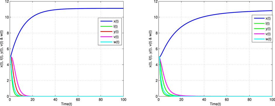
FIGURE 1. Time trajectories for uninfected cells x(t), latently infected cells l(t), infected cells y(t), viruses v(t), and antibodies w(t) of Eq. 2 with α = 1 (left banner) and α = 0.9 (right banner) and ${\mathcal{R}}_0=0.93<1$.

FIGURE 2

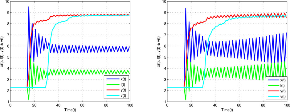
FIGURE 2. Time trajectories for uninfected cells x(t), latently infected cells l(t), infected cells y(t), and viruses v(t) of Eq. 2 with τ = 14 > τ* = 13.5, α = 0.9 (left banner) and α = 0.8 (right banner).

FIGURE 3

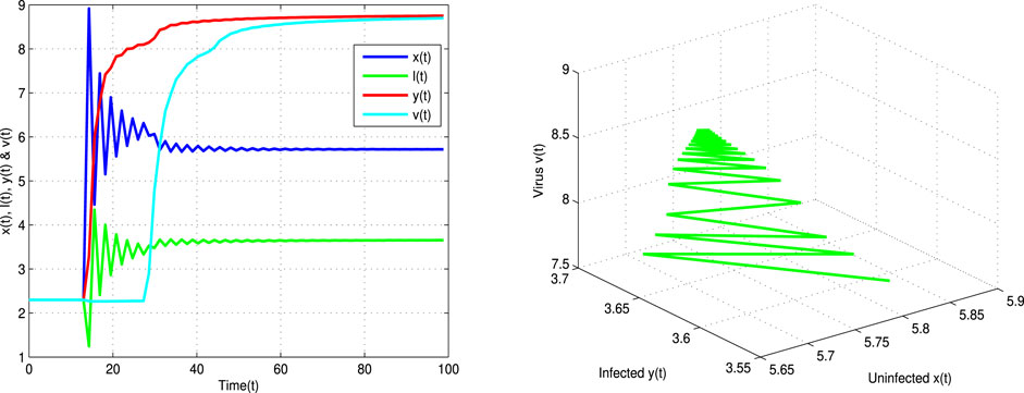
FIGURE 3. Time and space plane trajectories for uninfected cells x(t), latently infected cells l(t), infected cells y(t), and viruses v(t) of Eq. 2 with τ = 13 < τ* = 13.5 and α = 0.9.

Figure 4 displays the time trajectories of the considered model (2), which converge to the endemic equilibrium point ${\mathcal{E}}_2$, and stable behavior, when τ = 13 < τ* = 13.5. By increasing the fractional-order values, the curves get more flat and have significant effects on the cell dynamics.

FIGURE 4

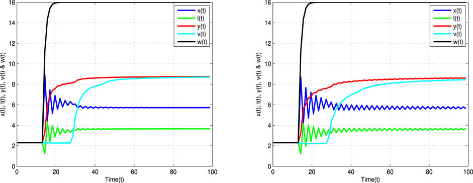
FIGURE 4. Time trajectories for uninfected cells x(t), latently infected cells l(t), infected cells y(t), viruses v(t), and antibodies w(t) of Eq. 2 with τ = 13 < τ* = 13.5, α = 0.9 (left banner) and α = 0.8 (right banner).

Remark 2. These are the results from the fractional-order viral infection model with latent infection and delay, which are different, complement, and expand upon those in [7,9,12]. The fractional-order stability regions in Figures 1–4 are larger than the corresponding integer-order stability regions in [7,12]. In a fractional-order model, the unstable equilibrium of an integer-order model may be a stable model. Furthermore, time-delays enhance the dynamics of the model and increase its complexity.

6 Concluding Remarks

Although the classical integer-order differential models can be useful for the study of disease dynamics, the fractional-order models are more useful for exploring disease dynamics. Several factors contribute to this, including data fitting, memory effects, and crossover effects. The fractional calculus is a powerful tool to describe physical and biological systems that have long-term memory and long-range spatial interactions. This paper examines the global dynamics of a fractional-order viral infection model with latent infection. We studied the positivity and boundedness of the solutions. Based on this formula, we derived the basic reproductive number ${\mathcal{R}}_0$, which acts as a threshold parameter in the viral infection disease status. For such a model, we examined the existence of equilibrium points and their corresponding asymptotic stability. Hopf bifurcation occurs at the critical values of the time-delay τ*. The Lyapunov–LaSalle method is used to determine the global stability of the model. A numerical solution for the proposed fractional-order viral infection model is obtained by employing Euler’s implicit scheme. Fractional order and time-delays increase the complexity and enrich the dynamics of the model.

Data Availability Statement

The original contributions presented in the study are included in the article/Supplementary Materials, and further inquiries can be directed to the corresponding author.

Author Contributions

FR was involved in project conceptualization and supervision, writing the original draft, and reviewing and editing the paper. CR was responsible for data visualization and validation, running the software, and performing the methodology.

Funding

This research was funded by UAE University, fund # 12S005-UPAR 2020.

Conflict of Interest

The authors declare that the research was conducted in the absence of any commercial or financial relationships that could be construed as a potential conflict of interest.

Publisher’s Note

All claims expressed in this article are solely those of the authors and do not necessarily represent those of their affiliated organizations, or those of the publisher, the editors, and the reviewers. Any product that may be evaluated in this article, or claim that may be made by its manufacturer, is not guaranteed or endorsed by the publisher.

References

1. Kang, C, Miao, H, and Chen, X. Global Stability Analysis for a Delayed Hiv Infection Model with General Incidence Rate and Cell Immunity. Engin Lett (2016) 24:392–8.

Google Scholar

2. Rihan, FA, and Velmurugan, G. Dynamics and Sensitivity of Fractional-Order Delay Differential Model for Coronavirus (Covid-19) Infection. Prog Fractional Differ Appl (2021) 7:43–61.

Google Scholar

3. Rihan, FA, and Alsakaji, HJ. Dynamics of a Stochastic Delay Differential Model for COVID-19 Infection with Asymptomatic Infected and Interacting People: Case Study in the UAE. Results Phys (2021) 28:104658. doi:10.1016/j.rinp.2021.104658

PubMed Abstract | CrossRef Full Text | Google Scholar

4. Dahari, H, Lo, A, Ribeiro, RM, and Perelson, AS. Modeling Hepatitis C Virus Dynamics: Liver Regeneration and Critical Drug Efficacy. J Theor Biol (2007) 247:371–81. doi:10.1016/j.jtbi.2007.03.006

CrossRef Full Text | Google Scholar

5. Yousfi, N, Hattaf, K, and Tridane, A. Modeling the Adaptive Immune Response in HBV Infection. J Math Biol (2011) 63:933–57. doi:10.1007/s00285-010-0397-x

CrossRef Full Text | Google Scholar

6. Stilianakis, N, and Seydel, J. Modeling the T-Cell Dynamics and Pathogenesis of Htlv-I Infection. Bull Math Biol (1999) 61:935–47. doi:10.1006/bulm.1999.0117

PubMed Abstract | CrossRef Full Text | Google Scholar

7. Wang, X, Tang, S, Song, X, and Rong, L. Mathematical Analysis of an Hiv Latent Infection Model Including Both Virus-To-Cell Infection and Cell-To-Cell Transmission. J Biol Dyn (2017) 11:455–83. doi:10.1080/17513758.2016.1242784

CrossRef Full Text | Google Scholar

8. Wen, Q, and Lou, J. The Global Dynamics of a Model about Hiv-1 Infection In Vivo. Ricerche mat. (2009) 58:77–90. doi:10.1007/s11587-009-0048-y

CrossRef Full Text | Google Scholar

9. Pan, S, and Chakrabarty, SP. Threshold Dynamics of Hcv Model with Cell-To-Cell Transmission and a Non-cytolytic Cure in the Presence of Humoral Immunity. Commun Nonlinear Sci Numer Simulat (2018) 61:180–97. doi:10.1016/j.cnsns.2018.02.010

CrossRef Full Text | Google Scholar

10. Elaiw, AM, and AlShamrani, NH. Global Properties of Nonlinear Humoral Immunity Viral Infection Models. Int J Biomath (2015) 08:1550058. doi:10.1142/s1793524515500588

CrossRef Full Text | Google Scholar

11. Luo, Y, Zhang, L, Zheng, T, and Teng, Z. Analysis of a Diffusive Virus Infection Model with Humoral Immunity, Cell-To-Cell Transmission and Nonlinear Incidence. Physica A: Stat Mech its Appl (2019) 535:122415. doi:10.1016/j.physa.2019.122415

CrossRef Full Text | Google Scholar

12. Wang, Y, Lu, M, Lu, M, and Jiang, D. Viral Dynamics of a Latent Hiv Infection Model with Beddington-Deangelis Incidence Function, B-Cell Immune Response and Multiple Delays. Mbe (2021) 18:274–99. doi:10.3934/mbe.2021014

CrossRef Full Text | Google Scholar

13. Hattaf, K. Global Stability and Hopf Bifurcation of a Generalized Viral Infection Model with Multi-Delays and Humoral Immunity. Physica A: Stat Mech its Appl (2020) 545:123689. doi:10.1016/j.physa.2019.123689

CrossRef Full Text | Google Scholar

14. Kilbas, AA, Srivastava, HM, and Trujillo, JJ. Theory and Applications of Fractional Differential Equations. North Holland Mathematics Studies, Vol. 204. Amsterdam: Elsevier Science (2006).

Google Scholar

15. Podlubny, I. Fractional Differential Equations. USA: Academic Press (1999).

Google Scholar

16. Rihan, FA. Delay Differential Equations and Applications to Biology. Singapore: Springer (2021).

Google Scholar

17. Rakkiyappan, R, Preethi Latha, V, and Rihan, FA. A Fractional-Order Model for Zika Virus Infection with Multiple Delays. Complexity (2019) 4178073. doi:10.1155/2019/4178073

CrossRef Full Text | Google Scholar

18. Latha, VP, Rihan, FA, Rakkiyappan, R, and Velmurugan, G. A Fractional-Order Model for Ebola Virus Infection with Delayed Immune Response on Heterogeneous Complex Networks. J Comput Appl Math (2018) 339:134–46. doi:10.1016/j.cam.2017.11.032

CrossRef Full Text | Google Scholar

19. Rihan, FA, Arafa, AA, Rakkiyappan, R, Rajivganthi, C, and Xu, Y. Fractional-order Delay Differential Equations for the Dynamics of Hepatitis C Virus Infection with IFN-α Treatment. Alexandria Eng J (2021) 60:4761–74. doi:10.1016/j.aej.2021.03.057

CrossRef Full Text | Google Scholar

20. Tamilalagan, P, Karthiga, S, and Manivannan, P. Dynamics of Fractional Order Hiv Infection Model with Antibody and Cytotoxic T-Lymphocyte Immune Responses. J Comput Appl Math (2021) 382:113064. doi:10.1016/j.cam.2020.113064

CrossRef Full Text | Google Scholar

21. Naik, PA, Zu, J, and Owolabi, KM. Global Dynamics of a Fractional Order Model for the Transmission of Hiv Epidemic with Optimal Control. Chaos, Solitons & Fractals (2020) 138:109826. doi:10.1016/j.chaos.2020.109826

CrossRef Full Text | Google Scholar

22. Danane, J, Allali, K, and Hammouch, Z. Mathematical Analysis of a Fractional Differential Model of Hbv Infection with Antibody Immune Response. Chaos Solitons Fractals (2020) 136:109787. doi:10.1016/j.chaos.2020.109787

CrossRef Full Text | Google Scholar

23. Shi, R, Lu, T, and Wang, C. Dynamic Analysis of a Fractional-Order Delayed Model for Hepatitis B Virus with Ctl Immune Response. Virus Res (2020) 277:197841. doi:10.1016/j.virusres.2019.197841

PubMed Abstract | CrossRef Full Text | Google Scholar

24. Wang, K, Wang, W, and Liu, X. Global Stability in a Viral Infection Model with Lytic and Nonlytic Immune Responses. Comput Math Appl (2006) 51:1593–610. doi:10.1016/j.camwa.2005.07.020

CrossRef Full Text | Google Scholar

25. Wang, K, Wang, W, and Liu, X. Viral Infection Model with Periodic Lytic Immune Response. Chaos, Solitons & Fractals (2006) 28:90–9. doi:10.1016/j.chaos.2005.05.003

CrossRef Full Text | Google Scholar

26. Wang, X, and Wang, W. An Hiv Infection Model Based on a Vectored Immunoprophylaxis experiment. J Theor Biol (2012) 313:127–35. doi:10.1016/j.jtbi.2012.08.023

CrossRef Full Text | Google Scholar

27. Wodarz, D. Hepatitis C Virus Dynamics and Pathology: The Role of Ctl and Antibody Responses. J Gen Virol (2003) 84:1743–50. doi:10.1099/vir.0.19118-0

CrossRef Full Text | Google Scholar

28. Song, X, Wang, S, and Dong, J. Stability Properties and Hopf Bifurcation of a Delayed Viral Infection Model with Lytic Immune Response. J Math Anal Appl (2011) 373:345–55. doi:10.1016/j.jmaa.2010.04.010

CrossRef Full Text | Google Scholar

29. Murase, A, Sasaki, T, and Kajiwara, T. Stability Analysis of Pathogen-Immune Interaction Dynamics. J Math Biol (2005) 51:247–67. doi:10.1007/s00285-005-0321-y

CrossRef Full Text | Google Scholar

30. Atangana, A. Derivative with a New Parameter: Theory, Methods and Applications. Academic Press (2015).

Google Scholar

31. Odibat, ZM, and Shawagfeh, NT. Generalized taylors Formula. Appl Math Comput (2007) 186:286–93.

CrossRef Full Text | Google Scholar

32. Sardar, T, Rana, S, Bhattacharya, S, Al-Khaled, K, and Chattopadhyay, J. A Generic Model for a Single Strain Mosquito-Transmitted Disease with Memory on the Host and the Vector. Math Biosciences (2015) 263:18–36. doi:10.1016/j.mbs.2015.01.009

CrossRef Full Text | Google Scholar

33. Sardar, T, Rana, S, and Chattopadhyay, J. A Mathematical Model of Dengue Transmission with Memory. Commun Nonlinear Sci Numer Simulation (2015) 22:511–25. doi:10.1016/j.cnsns.2014.08.009

CrossRef Full Text | Google Scholar

34. van den Driessche, P, and Watmough, J. Reproduction Numbers and Sub-threshold Endemic Equilibria for Compartmental Models of Disease Transmission. Math Biosci (1802) 180:29–48. doi:10.1016/s0025-5564(02)00108-6

CrossRef Full Text | Google Scholar

35. Beretta, E, and Kuang, Y. Geometric Stability Switch Criteria in Delay Differential Systems with Delay Dependent Parameters. SIAM J Math Anal (2002) 33:1144–65. doi:10.1137/s0036141000376086

CrossRef Full Text | Google Scholar

36. Li, H-L, Zhang, L, Hu, C, Jiang, Y-L, and Teng, Z. Dynamical Analysis of a Fractional-Order Predator-Prey Model Incorporating a Prey Refuge. J Appl Math Comput (2017) 54:435–49. doi:10.1007/s12190-016-1017-8

CrossRef Full Text | Google Scholar

37. Sene, N. Stability Analysis of the Fractional Differential Equations with the Caputo-Fabrizio Fractional Derivative. J Fract Calculus Appl (2020) 1:160–72.

Google Scholar

38. Rihan, FA, Lakshmanan, S, Hashish, AH, Rakkiyappan, R, and Ahmed, E. Fractional-order Delayed Predator-Prey Systems with Holling Type-II Functional Response. Nonlinear Dyn (2015) 80:777–89. doi:10.1007/s11071-015-1905-8

CrossRef Full Text | Google Scholar