Identifying Actionable Serial Correlations in Financial Markets

1 Introduction

In his seminal 1970 paper, Fama introduced the notion of an efficient market, within which the prices of securities fully reflect all information from the past, as well as future expectations on their returns [1]. In his paper, the empirical evidence Fama cited as supporting this efficient market hypothesis is zero (or close to zero) serial correlation. However, if financial markets are truly efficient, then it would be impossible for traders to profit beyond the fundamental values of the securities. Naturally, the only trading strategy that makes sense in an efficient market would be buy-and-hold. This brings us then to the elephant in the room: why are there so many hedge funds (according to https://www.investopedia.com/terms/h/hedgefund.asp, more than 10,000 of them) in the world, and why are so many of them making money? Fundamentally, all hedge funds engage in some form of technical trading [2–4], frequently dismissed by financial economists as not founded on firm principles. The profitability of technical trading was first investigated by Lukac et al. [5] and Brock et al. [6]. Testing 12 technical trading rules for 12 commodities between 1978 and 1984, Lukac et al. found that seven rules produced significant gross returns, while four rules produced significant net returns and significant risk-adjusted returns, after taking into account transportation and storage costs. Testing the commonly used moving average and trading range break rules on the Dow Jones index from 1897 to 1986, Brock et al. found these technical trading rules generating significant positive returns, especially from buy signals. Later, Levich and Thomas [7], Parisi and Vasquez [8], Kwon and Kish [9], also showed that technical trading can be significantly profitable, for currency futures contracts between 1976 and 1990, for many stocks on the Chilean stock market between 1989 and 1998, and for the New York Stock Exchange value-weighted index over the period 1962 to 1996, respectively.

When the technical trading rules were tested within shorter subperiods in Refs. [7] and [9], their profitabilities were found to be lower for the last sub-periods, 1986 to 1990 and 1985 to 1996, respectively. Kwon and Kish suspected that this was due to the market becoming more efficient after computerization. But as they pondered this, a wave of criticism on technical trading started, led by the papers by Ready [10] and Bajgrowicz and Scaillet [11]. In these papers, as well as those by Fang et al. [12] and Taylor [13], technical trading rules found to be profitable in the earlier periods in Ref. [6] were tested for later periods, and found to have lost their magic. Taylor, who examined the performance of momentum-based technical trading rules over the cross section of Dow Jones Industrial Average component stocks between 1928 and 2012, found the profitability of these technical trading rules evolving slowly over time, but are most profitable between the mid-1960s to the mid-1980s. This phenomenon was also observed for the performance of hedge funds. For example, earlier studies by Ackermann et al. and Liang reported stellar performances of 9.2–16.1% annual return for 906 hedge funds between January 1994 and December 1995) [14], and monthly returns ranging from $-0.10$ to $+1.35\%$ for 385 hedge funds between January 1994 and December 1996 [15], respectively. However, a more recent study by Fung et al. of 1,603 funds between January 1995 and December 2004 found them delivering 14–24% annual return only between 1995 and 1999 [16]. In 1998, the average return was zero, presumably because of the Long Term Capital Management crisis, and generally anemic from 2000 onwards (except for 12% in 2003), because of the NASDAQ crash in 2000. In principle, these criticisms focused on technical trading rules shown to be profitable in earlier papers, and therefore do not constitute definitive proof that technical trading rules as a whole do not work. For example, it is entirely possible that some rules work well in a given period, but as they becomes less effective in another period, other rules would become more profitable. It is also possible, while a technical trading rule is profitable in a given period, another rule that we have not considered might do even better. This last problem of finding the optimal technical trading rule based on hidden temporal patterns is one ideally suited to machine learning. In one of the earliest studies, Allen and Karjalainen used a genetic algorithm to learn technical trading rules for the daily S&P 500 prices from 1928 to 1995 [17]. Unfortunately, the rules learned did not perform better than the simple buy-and-hold strategy in out-of-sample test periods, although some rules did performed better in some periods. Fernández-Rodríguez et al. had better luck, finding that the simple technical trading rule is superior to the buy-and-hold strategy for bear and bull markets [18].

Ultimately, through the literature survey above, we see that machine learning is also not exhaustive. It finds the best, but not all that are profitable. Also, technical trading rules discovered through machine learning (including those using artificial neural networks [19–21]) do not necessarily perform better than those learned by human traders. Here let us address the question why technical trading rules have only short-lived successes, from the context of information processing by complex systems. For example, a typical language like English contains more than 100,000 words, using which we construct sentences containing about 20 words. However, an overwhelming majority of the ${20}^{{10}^5}$ sentences that we form by randomly selecting words are unintelligible. For an English sentence to be meaningful, the sequence of words has to closely obey a set of rules that we call the English grammar, and further constrained to convey meaning. Because of this severe reduction of the space of all possible sentences to the space of all meaningful sentences, we expect in daily usage many sentences or sub-sentences to be repeated. Another way to look at this phenomenon, is that recurrent sequences are necessary for the transmission of meaning or information, and for information processing in general. Consequently, the rules of the language make it more likely for repetition to occur. Another example of information processing in complex systems is the Krebs cycle in our biological pathways, which gets activated more than ${10}^{13}$ times a day to produce adenosine triphospate (ATP) [22, 23], a molecule that we constantly consume to stay alive. If we could measure the concentrations of all transcribed species, the highly recurrent sequences associated with the Krebs cycle would be impossible to miss.

Financial markets are also complex systems, in which participants are constantly learning how to process the complex information coursing through the system. As they do so, they add to the complex information in the system. Therefore, efficient or not, we expect hidden rules and recurrent sequences to be present in financial markets. However, as financial agents act on the market, they are themselves acted upon. As such, no agent or strategy can dominate forever, even though a previously-dominant strategy may return to dominance time and again. This explains why technical trading rules can be profitable (because exploitable information always exists in the market), and why their profitabilities are short-lived (because they generate information that can be exploited by other technical trading rules). Therefore, when a group of technical trading rules become unprofitable, another group of technical trading rules become profitable. This tells us that to hunt for this shifting information, we should look not only for correlations in time, but also correlations in space, across different instruments and different asset classes. So far, technical trading focuses on temporal patterns representing high-order serial correlations in individual instruments, but spatio-temporal patterns involving multiple instruments should also exist, and can be exploited for technical trading. Surprisingly, after a broad survey of the literature, we found no previous studies on technical trading based on spatio-temporal patterns. In fact, when we search Google Scholar using “pattern recognition” and “multivariate time series”, we end up with two hits. In the 2011 conference paper by Spiegel et al. [24], time series segmentation was first used to define features in the individual time series, before these features were used to define patterns across the small number of car accelerator sensor time series. In their 2016 paper [25], Fontes and Pereira used a three-step method involving subsequence matching and fuzzy clustering, followed by PCA to analyze sensor time series cross section from a gas turbine for monitoring and fault prediction.

In this paper, we take the natural next step to test the feasibility of technical trading using spatio-temporal patterns over the cross section of Dow Jones Industrial Average component stocks, as well as over cross sections of multiple asset classes including commodities, bonds, FOREX rates, indices, metals, and oil and gas. To find these recurrent spatio-temporal patterns, all these existing works relied on time series segmentation to first convert a real-valued time series into a symbolic time series. This is computationally heavy, so instead of time series segmentation, we describe in Section 2 how we collected and cleaned our data, and how we map a specific choice of price movements to spatio-temporal cross sections of strings with lengths up to 5 days and comprising up to 10 alphabets. Ultimately, with this symbolic mapping all temporal patterns can be mapped to strings of alphabets. However, even after this simplification the extraction of actionable information on financial markets is not a trivial task, firstly because we have no prior knowledge what these signals would look like, and must thus analyze movements within the system, identify recurrent sequences that appear, and use these to infer the rules of information processing within financial markets. Such an analysis has been carried out in various fields to analyze various complex systems [26–30], and we ourselves have done so for natural languages [31] and teaching practices [32]. Secondly, the very many signals overlap in time to mask each other, and more importantly, participants hide their intentions as they trade. This leads to the financial markets becoming so “noisy” that one can guess price movements correctly only slightly more than 50% of the time (although Kelly showed in 1956 that this is sufficient to ensure a positive return betting on an outcome [33]). This second problem also occurs for our gene expression machinery, or the information processing machinery of other complex systems. Fortunately, network science has made great strides in systematically and independently identifying spatial motifs [34–36], which are collections of nodes that are co-activated much more frequently than we expected from random and uncorrelated activation of nodes, or temporal motifs [37, 38], which are sequences of nodes that are activated one after another. Spatial motifs can be very large, and we need a lot of data to be confident that they are not products of random fluctuations. Similarly, temporal motifs can be very long, making the space of sequences to search through very large indeed. As far as we know, there have been no efforts to develop methods for identifying spatio-temporal motifs, consisting of different cross sections of nodes at different lags. Therefore, in Section 2, we describe how to unpack spatio-temporal sequences into collections of temporal sequences, and thereafter test these empirical sequences against null models to identify sequences that are repeated more frequently than by chance. We then report in Section 3 that in general, there are no actionable serial correlations for single instruments, but many recurrent multiple-instrument spatio-temporal sequences exist, which allow one to design trading strategies around them. Finally, we tested the feasibility of these trading strategies in Section 4, before summarizing our findings in Section 5.

2 Data and Methods

2.1 Data

We downloaded two sets of time series data in the form of comma-separated values (CSV) files. The first set (see Supplementary Table S1) comprised daily prices of the 30 component stocks of the Dow Jones Industrial Average (DJI). These belong to the 30 largest publicly-owned United States companies, which are prominent brand names many people are familiar with. We used the maximum time period for each stock, so that we can compare them across the longest possible time period. The second set (see Supplementary Table S2) comprised daily prices of three to five instruments each from six different asset classes, including stock indices, precious metals, commodities, government bonds, energy materials, and foreign exchange. The 26 instruments in this second data set were selected primarily because data was readily available, and also because they are easily recognizable.

We then imported these CSV files into Python for cleaning. First, we removed empty cells or cells that contain errors, before saving the cleaned data as two separate numpy files. The first file contains the dates in International Organization for Standardization (ISO) format, while the second file contains the corresponding closing prices. For missing prices over weekends or public holidays, we set them equal to the prices of the previous days. As such, a financial instrument can only increase continuously for at most 5 days, as closing prices over the weekends are set to those on Friday.

2.2 Compiling Lists of Spatio-Temporal Sequences

To avoid having to deal with the full complexity of financial markets, but still be able to discover statistically significant patterns within the data, we map the day-to-day price change time series to symbolic sequences from a small alphabet. There are many ways this can be done, depending on what trading strategy we would like to adopt. For example, if we would like to watch for 2 days of positive price changes, and buy the instruments that are most likely to also experience positive price changes in the next one, two, or three days, we would choose to map the price changes to letters of an alphabet (one letter for each instrument), only when the price changes are positive. This example is illustrated in Figure 1A. Alternatively, if we would like to sell an instrument whose price is most likely to fall after 2 days of gain in the prices of two other instruments, we can map positive price changes to uppercase letters ‘A’, ‘B’, ‘C’, …, and negative price changes to lowercase letters ‘a’, ‘b’, ‘c’, ….

FIGURE 1

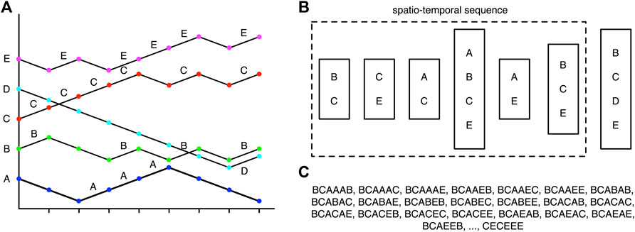
FIGURE 1. (A) The price time series of five financial instruments, mapped to the alphabets ‘A’, ‘B’, ‘C’, ‘D’, ‘E’. When the price of an instrument rises, the corresponding letter is added to the spatial cross section. (B) For days $t=1$ to $t=6$, the spatial cross sections are non-empty, but there are no price gains on day $t=7$ (and therefore the spatial cross section on this day is empty). Thereafter, on day $t=8$, we find a new non-empty spatial cross section. Hence we find a length-6 spatio-temporal sequence (of non-empty spatial cross sections) that ends on day $t=6$, and another spatio-temporal sequence starting on day $t=8$. In practice, because we set the price on a non-trading day to the price on the last trading day, the longest spatio-temporal sequence we have to deal with in this paper is length-5. (C) The length-6 spatio-temporal sequence shown in (B) can also be thought of as being equivalent to $2\times 2\times 2\times 4\times 2\times 3=192$ length-6 temporal sequences. Some of these temporal sequences are shown here.

In Figure 1B, we show how we organize the symbolic sequences of the cross section of instruments into spatio-temporal sequences. A spatio-temporal sequence consists of spatial cross sections like (‘B’, ‘C’), (‘C’, ‘E’), (‘A’, ‘C’), (‘A’, ‘B’, ‘C’, ‘E’), (‘A’, ‘E’), (‘B’, ‘C’, ‘E’) at successive times. Spatial cross sections at different times need not be the same in size, like (‘B’, ‘C’) and (‘A’, ‘B’, ‘C’, ‘E’) for example. Spatio-temporal sequences also need not be equally long in time. For example, the spatio-temporal sequence (‘B’, ‘C’) → (‘C’, ‘E’) → (‘A’, ‘C’) → (‘A’, ‘B’, ‘C’, ‘E’) → (‘A’, ‘E’) → (‘B’, ‘C’, ‘E’) has a temporal length of 6. This spatio-temporal sequence stops here, because in the time series cross section, no instrument has an increasing price on day 7. The spatial cross section (‘B’, ‘C’, ‘D’, ‘E’) on day 8 then represents the start of the next spatio-temporal sequence, which may have a different temporal length. Going through the time series cross section $\left\{\left(\Delta p_{\mathrm{1,1}},\dots ,\Delta p_{1,t},\dots ,\Delta p_{1,T}\right),\dots ,\left(\Delta p_{N,1},\dots ,\Delta p_{N,t},\dots ,\Delta p_{N,T}\right)\right\}$, where $\text{Δ}{p}_{i,t}$ is the price change of instrument $i=1,\dots ,N$ on day $t=1,\dots ,T$, we then obtain a list of spatio-temporal sequences $\left\{{\Sigma }_1,\dots ,{\Sigma }_k,\dots ,{\Sigma }_n\right\}$, where ${\text{Σ}}_k={\sigma }_{k,1}\to {\sigma }_{k,2}\to \cdots \to {\sigma }_{k,m_k}$ consists of $m_k$ spatial cross sections ${\sigma }_l=\left(s_{l,1},s_{l,2},\dots ,s_{l,p_l}\right)$. In spatial cross section ${\sigma }_l$, the price changes of $1\le p_l\le N$ instruments (whose symbols are $s_{l,1},\dots ,s_{l,p_l}$) are positive.

2.3 Null Model and Test of Statistical Significance

In general, when we expand the spatio-temporal sequences into temporal sequences, and count the number of times they appear, some temporal sequences will be frequent, while others will be rare. However, a frequent temporal sequence may be less informative than a rare temporal sequence, if the former contains many highly-frequent symbols. In other words, these frequent temporal sequences can occur by chance, because their symbols are so common. Therefore, the frequencies of different temporal sequences must be tested against appropriate null models, to ensure at the very least that they are not likely to be obtained by chance.

Depending on what information we are interested in, we can construct different null models. In Section 3.1, we will show that the probability of empirically finding positive price movements in an instrument for r consecutive days is $p^r$, where p is the probability of finding positive price movement for the instrument on any given day. This suggests that the appropriate null model to use for one instrument is independent price movements on each day. We can of course use this same null model for all N instruments. However, in this null model the N instruments would be uncorrelated in time (between different time lags) and also in space (between different instruments), when strong cross correlations between instruments are well known. Using such a null model, we will find many statistically significant spatio-temporal sequences with strong cross correlations between instruments on the same days. There is no gain trading these spatio-temporal sequences, since we cannot act on strong cross correlations within the same day. Therefore, we should choose a different null model that does not throw the baby out with the bath water.

A simple null model that preserves spatial cross correlations, but contains no temporal correlations, can be obtained by reshuffling the empirical spatio-temporal sequences, as shown in Figure 2. If this reshuffling is done within individual spatio-temporal sequences, we also preserve the distribution of lengths. With this null model, and some additional care, it is even possible to perform statistical testing at the level of spatio-temporal sequences. However, we chose for simplicity to perform statistical testing at the level of temporal sequences. A temporal sequence is a simple word (string of symbols), like ‘BCA’, ‘BCABA’, and so on. To do the test, we extract all possible words that can be generated from the list of spatio-temporal sequences. For example, for (‘B’, ‘C’) → (‘C’, ‘E’) → (‘A’, ‘C’), we can generate the words ‘BCA’, ‘BCC’, ‘BEA’, ‘BEC’, ‘CCA’, ‘CCC’, ‘CEA’, ‘CEC’. We then count the number of times each word appears after this unpacking of the spatio-temporal sequences. These are our empirical frequencies.

FIGURE 2

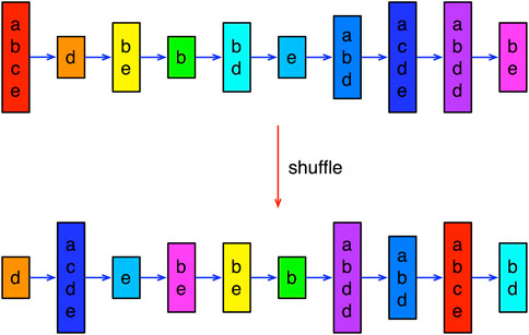
FIGURE 2. Shuffling a length-10 spatio-temporal sequence with spatial cross sections of different sizes, to obtain a null-model ensemble of length-10 spatio-temporal sequences.

Next, we shuffle the empirical spatio-temporal sequences $S=100$ times to create an ensemble of null-model spatio-temporal sequences. For a spatio-temporal sequence of length $m_k$, we can generate up to $m_k!$ null-model spatio-temporal sequences. Some short spatio-temporal sequences with $m_k<5$ will be repeated if we shuffle them $S=100$ times, but we need not worry about repetitions even if the data contains just $n=10$ spatio-temporal sequences, as there will be ${\langle m!\rangle }^n\sim {10}^{17}$ distinct combinations if $\langle m!\rangle =50$ is the average number of null-model spatio-temporal sequences that can be generated from each empirical spatio-temporal sequence. Since we shuffle the empirical spatio-temporal sequences $S=100$ times, after unpacking the null-model spatio-temporal sequences into temporal sequences, and counting the number of times different words appear, we will have a distribution of $S=100$ null-model frequencies for each word.

Since we sampled the null model $S=100$ times, it is convenient for us to perform the statistical test at the level $p<0.01$. A word that is significant at this level would have an empirical frequency that is larger than all $S=100$ null-model frequencies. Also, because the null-model frequencies of all words are obtained simultaneously from the shuffling of spatio-temporal sequences, we do not need to make Bonferroni [39] or similar corrections [40] for the multiple comparisons that we are making. All statistically significant words will truly be at the $p<0.01$ level of confidence. In a sense, by testing observations against the null model, we are simultaneously testing all kinds of autocorrelations and cross correlations between the sign time series of the various instruments.

3 Results

3.1 1-Letter Words

When we analyze each of the 56 instruments independently, by emitting a single letter when the price increases, we are looking at bull runs of different durations in their time series. We show the distributions of durations for stocks in the first data set in Supplementary Figure S1, and those for instruments in the second data set in Supplementary Figure S2. Plotted on a linear-log scale, these graphs are all close to being linear, suggesting that the distributions are exponential. Such an exponential distribution arises very naturally if we assume that the price increase on one day is uncorrelated with a price increase on any other day. Therefore, if the probability of a price increase is p, the probability of finding a bull run over r days is simply

$p^r=\exp \left(r\ln p\right)=\exp \left(-r\left|\ln p\right|\right).(1)$

This result should not surprise us, since it is just an unconventional way to present a very well known observation in finance, namely the serial correlation or autocorrelation is nearly zero [41]. This also means that there is no signal for a trader to act on, when the 1-letter word lengths are so distributed, beyond betting on the probability p of getting a price increase on a given day, regardless of the number of days of price increases prior to it. According to Fama and others after him, the market is thus “efficient” [1].

3.2 2-Letter Words

However, this does not mean that there is no actionable price movement information in the financial markets. In fact, trying to understand this information by looking at the price movement of a single instrument is like trying to understand the first sentence of this paragraph by looking at the distribution {_,_, _, ‘a’, ‘a’, _, _, _, ‘aa’, _, _, ‘a’, _, _, ‘aa’, ‘a’} of the letter ‘a’ appearing in the words. If we use two letters, say ‘a’ and ‘e’, the distribution {‘ee’, _, ‘e’, _, ‘ea’, ‘a’, ‘ee’, _, _, ‘aae’, ‘e’, ‘ee’, ‘a’, _, ‘e’, ‘aa’, ‘ae’} is now more informative (though still not enough for us to comprehend the sentence). The distribution {‘ee’, ‘i’, ‘e’, _, ‘ea’, ‘a’, ‘ee’, ‘i’, _, ‘aiae’, ‘ie’, ‘ee’, ‘iai’, ‘i’, ‘e’, ‘iaia’, ‘ae’} becomes even more informative if we include one more letter (‘i’). In this subsection, let us demonstrate (as a proof of concept) how we can extract more information from the distribution of 2-letter words. To do this, let us examine two pairs of instruments, (A = HD, B = TRV) and (A = platinum, B = USD-EUR), which are chosen because individually, their distributions of 1-letter words are the least informative (in that the probability of finding a word with length-r is closest to the product of independently finding r length-1 words).

For the HD-TRV pair, we used data between Sep 22, 1981 and Mar 7, 2018. Going through the 9,194 closing prices, we found 1,019 trading days when there were no price increases in either HD or TRV. The rest of the trading days are partitioned into 1,974 spatio-temporal sequences. The shortest of these spatio-temporal sequences are {(A)}, {(B)}, and {(A, B)}, which are the three possible spatial cross-sections. The longest spatio-temporal sequence is length-22 (price increases over multiple holidays and weekends). We focused on the 1,676 spatio-temporal sequences length-5 and shorter. These unpack into 4,213 temporal sequences, with the distribution shown in Table 1. As expected, after statistical testing at the level of $p<0.01$ most of the temporal sequences are insignificant, except for BABA and BABB. This tells us that after a price increase in TRV on day 1, followed by a price increase in HD on day 2, followed by a price increase in TRV on day 3, there is a very significant chance of price increases in either HD or TRV. We can find more actionable temporal sequences if we relax the criterion of our statistical testing to $p<0.05$.

TABLE 1

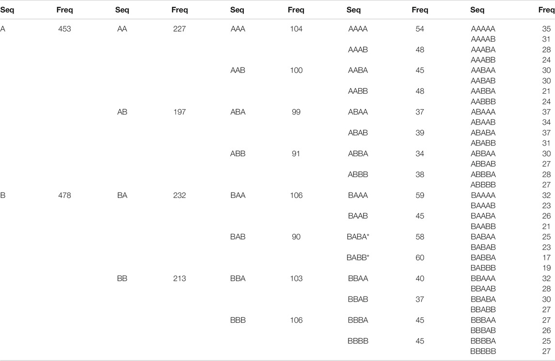
TABLE 1. Empirical frequencies of 2-letter temporal sequences of up to length-5, corresponding to price increases in HD and TRV. In this table, an asterix indicates statistical significance at the level of $p<0.01$.

For the platinum-USD-EUR pair, we used data between Dec 27, 1979 and Mar 13, 2018. Going through the 9,922 prices, we found 639 trading days when there were no price increases in either platinum or USD-EUR. The rest of the trading days were partitioned into 1,884 spatio-temporal sequences, and the longest spatio-temporal sequence is length-27 (price increases over multiple holidays and weekends). Focusing on the 1,449 spatio-temporal sequences length-5 and shorter, we find that these unpack into 3,185 temporal sequences, with the distribution shown in Table 2. In this case, we find BA occurring more frequently than expected from the null model, at the $p<0.01$ level. No other temporal sequences occur more frequently than expected from the null model, even at the $p<0.05$ level. This tells us that an increase in the USD-EUR exchange rate is very likely to be followed by an increase in the price in platinum the next day—an observation that traders can act on! Interestingly, ABBA, AAABB, and AAAAB occur less frequently than expected from the null model, the first two at the $p<0.05$ level, while the last at the $p<0.01$ level. The observations on AAABB and AAAAB suggest that following 3–4 days of increases in the platinum price, we are likely to find an ensuing decrease in the USD-EUR exchange rate. This is also an observation that traders can act on.

TABLE 2

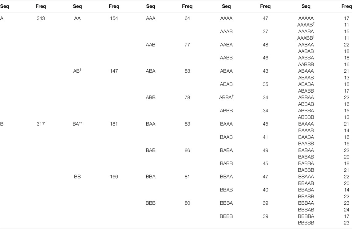
TABLE 2. Empirical frequencies of 2-letter temporal sequences of up to length-5, corresponding to price increases in platinum and USD-EUR. In this table, an empirical frequency that is significantly higher than expected from the null model is indicated by an asterix ($p<0.05$) or two asterixes ($p<0.01$), whereas an empirical frequency that is significantly lower than expected from the null model is indicated by a dagger ($p<0.05$) or a double dagger ($p<0.01$).

3.3 5-Letter Words

In Section 3.2, we illustrated how we can better understand the information contained in an English sentence by going from one-letter sequences to two-letter sequences, and how the information extraction improved with three-letter sequences. In this subsection, let us show that this is also true for financial markets, by going to a cross section of five stocks, (A) GE, (B) CSCO, (C) HD, (D) JPM, (E) MMM, using prices between Feb 16, 1990 and Mar 8, 2018. Out of the 10,248 trading days, there are 2,225 days on which there are no price increases in any of the five stocks. From the remaining 8,023 trading days, we found 1,987 spatio-temporal sequences of lengths between 1 and 5. After unpacking, we obtained 158,106 temporal sequences.

Out of $5+5^2+5^3+5^4+5^5=\mathrm{3,905}$ distinct five-letter temporal sequences of length up to 5, we found 183 temporal sequences $\left(<5\%\right)$ that are statistically significant at the level of $p<0.05$. Of these, 35 $\left(<1\%\right)$ are statistically significant at the level of $p<0.01$. These are not small numbers. The distributions of dynamical motifs are skewed in favor of longer temporal sequences. For the $p<0.05$ temporal sequences, four are length-2, five are length-3, 27 are length-4, and 147 are length-5. For the $p<0.01$ temporal sequences, one is length-3, five are length-4, and 29 are length-5. Therefore, the identification of longer dynamical motifs seems to be easier. However, they are also less common overall. For trading, a compromise has to be found.

For this cross section of five stocks, we also found a very interesting statistic: of the 183 $p<0.05$ temporal sequences, 39 starts with A (GE), 32 starts with B (CSCO), 27 starts with C (HD), 43 starts with D (JPM), and 42 starts with E (MMM). Restricting ourselves then to the 147 length-5 $p<0.05$ temporal sequences, we found that 22 ends with A (GE), 47 ends with B (CSCO), 42 ends with C (HD), 14 ends with D (JPM), and 22 ends with E (MMM). This suggests that, even though we only look at five stocks, JPM, MMM, and GE are leaders in market-wide bull runs (and thus less likely to follow), whereas CSCO and HD are followers (and thus less likely to lead).

Finally, we find 11 of the $p<0.05$ length-5 motifs containing ABB. These are ABABB, BAABB, CBABB, CCABB, DBABB, EAABB, EABBB, EBABB, ECABB, EDABB, EEABB. Apart from EABBB, ABB occurs at the end. This is an observation that traders can definitely act upon. However, since ABB is itself a $p<0.01$ length-3 motif, perhaps it is not surprising that we find these length-5 motifs extending ABB. The situation is different with CBB, whose empirical frequency is exceeded by 15 null-model frequencies ($p=0.15$), and thus not very significant. In spite of this, we find 8 length-5 motifs at $p<0.05$ containing CBB. These are ABCBB, ADCBB, CBBBB, EACBB, EBCBB, ECCBB, EDCBB, EECBB. Except in CBBBB, CBB again occurs at the end of the other motifs, making them actionable. More importantly, if we compare the two series of length-5 motifs,

$\begin{array}{l}\mathbf{AB}\text{ABB,}\text{BAABB,}\text{CBABB,}\text{CCABB,}\text{DBABB,}\mathbf{EA}\text{ABB,}\mathbf{EB}\text{ABB,}\mathbf{EC}\text{ABB,}\mathbf{ED}\text{ABB,}\mathbf{EE}\text{ABB;}\\ \mathbf{AB}\text{CBB,}\text{ADCBB,}\mathbf{EA}\text{CBB,}\mathbf{EB}\text{CBB,}\mathbf{EC}\text{CBB,}\mathbf{ED}\text{CBB,}\mathbf{EE}\text{CBB,}\end{array}$

we find that six prefixes match, and their empirical frequencies are close to each other. Therefore, we can write these 12 length-5 motifs as

$\text{AB}\left[\begin{array}{c}\text{ABB}\\ \text{CBB}\end{array}\right],\text{EA}\left[\begin{array}{c}\text{ABB}\\ \text{CBB}\end{array}\right],\text{EB}\left[\begin{array}{c}\text{ABB}\\ \text{CBB}\end{array}\right],\text{EC}\left[\begin{array}{c}\text{ABB}\\ \text{CBB}\end{array}\right],\text{ED}\left[\begin{array}{c}\text{ABB}\\ \text{CBB}\end{array}\right],\text{EE}\left[\begin{array}{c}\text{ABB}\\ \text{CBB}\end{array}\right],(2)$

and then further as

$\left[\begin{array}{c}\text{AB}\\ \text{EA}\\ \text{EB}\\ \text{EC}\\ \text{ED}\\ \text{EE}\end{array}\right]\left[\begin{array}{c}\text{ABB}\\ \text{CBB}\end{array}\right]=\left[\begin{array}{c}\text{AB}\\ \text{E}\left[\begin{array}{c}\text{A}\\ \text{B}\\ \text{C}\\ \text{D}\\ \text{E}\end{array}\right]\end{array}\right]\left[\begin{array}{c}\text{ABB}\\ \text{CBB}\end{array}\right].(3)$

In doing so, we are repacking the 12 length-5 temporal motifs back into a spatio-temporal motif.

3.4 10-Letter Words

Ultimately, there are tens of thousands of stocks on the New York Stock Exchange and other US exchanges, so the 30 DJI component stocks, or even the 500 S&P 500 component stocks cannot provide a comprehensive picture on all information flowing through these stock markets. If we go beyond stock markets, to include assets from other financial markets (commodities, oil and gas, bonds, foreign exchange, …), it is clear a cross section of five instruments represents not even the tip of an iceberg. It is thus tempting to consider cross sections of many more instruments. However, as we have seen from Section 3.2 and Section 3.3, while the numbers of spatio-temporal sequences remain comparable, the numbers of temporal sequences that we unpack going from a two-letter alphabet to a five-letter alphabet increased 50-fold. If we now go from a five-letter alphabet to a 10-letter alphabet, the numbers of temporal sequences is expected to increase another 30-fold, to approximately $5\times {10}^6$. If this number of temporal sequences gets any larger, testing them statistically will no longer be feasible on a desktop computer, so we must forget going to 50 letters (utilizing both uppercase and lowercase letters), where we would have to deal with $3\times {10}^8$ temporal sequences after unpacking, or larger alphabets.

At the same time, the information we can extract from financial markets become richer when we use larger alphabets. To illustrate this, and also highlight new problems encountered, let us analyze two large cross sections of instruments in this subsection: 1) a cross section of 10 DJI component stocks, and 2) a cross section of nine mixed assets. In the first cross section, (A) GE, (B) CSCO, (C) HD, (D) JPM, (E) MMM, (F) MRK, (G) UTX, (H) BA, (I) VZ, (J) XOM, we used prices between Feb 16, 1990 and Mar 8, 2018. Out of 10,248 trading days, we found 1,863 days on which there were no price increases in any of the stocks. For the rest of the trading days, price increases were organized into 1,738 spatio-temporal sequences up to length-5. For 10 stocks, there are 111,110 unique temporal sequences. Out of these, 3,580 temporal sequences are statistically significant at the $p<0.05$ level, while 672 are significant at the $p<0.01$ level. As functions of sequence length, these are distributed as

$\left(F_1,F_2,F_3,F_4,F_5\right)=\left(2,43,42,235,3258\right)(4)$

for $p<0.05$, and

$\left(F_1,F_2,F_3,F_4,F_5\right)=\left(0,20,3,33,616\right)(5)$

for $p<0.01$, where $F_n$ is the frequency of length-n dynamical motifs. Of the $p<0.05$ motifs,

$\begin{array}{l}\left(F_A^{pre},F_B^{pre},F_C^{pre},F_D^{pre},F_E^{pre},F_F^{pre},F_G^{pre},F_H^{pre},F_I^{pre},F_J^{pre}\right)\\ =\left(214,149,207,197,363,605,105,143,516,1081\right),\end{array}(6)$

where $F_{\sigma }^{pre}$ is the number of motifs starting with the letter $\sigma =$ A, …, J, whereas

$\begin{array}{l}\left(F_{5,\text{A}}^{post},F_{5,\text{B}}^{post},F_{5,\text{C}}^{post},F_{5,\text{D}}^{post},F_{5,\text{E}}^{post},F_{5,\text{F}}^{post},F_{5,\text{G}}^{post},F_{5,\text{H}}^{post},F_{5,\text{I}}^{post},F_{5,\text{J}}^{post}\right)\\ =\left(426,289,830,125,270,159,204,495,191,269\right),\end{array}(7)$

$F_{\sigma }^{post}$ being the number of motifs ending with the letter $\sigma =\text{A},\dots ,\text{J}$. This tells us that XOM, MRK, VZ, MMM are the top four leaders, while HD, BA, GE, CSCO, MMM are the top five followers. Again, leaders are not followers (with the exception of MMM).

Because of the number of $p<0.05$ motifs, we can no longer visually inspect individual sequences like we did for the 5-letter case to identify actionable patterns. This is why a visualization scheme is necessary. Since XOM is the strongest lead mover, we can choose to visualize only the 1,063 length-5 motifs that start with J, in the form of a tree rooted in J. From this root, we draw branches to the 10 letters in the first level (if such sequences exist), and from each of these letters, draw branches to the 10 letters in the second level (if such sequences exist), and so on and so forth until we reach the end of the sequences (the leaves). Because we draw only existing sequences, some branches will have more leaves while others will have fewer, as shown in Figure 3. The tree diagrams with other roots in this cross section of 10 DJI stocks are shown in Supplementary Figure S3. In Supplementary Figure S4, we also show the tree diagrams for a second cross section of 10 DJI stocks.

FIGURE 3

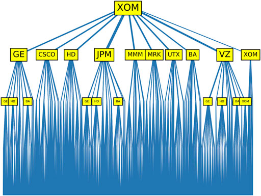
FIGURE 3. Tree diagram of dynamical motifs rooted in (J) XOM (price increase on the first day). In this figure, we label all ten stocks with price increases on the second day, but use a larger font for (A) GE, (D) JPM, and (I) VZ, to indicate that price increases in these stocks are followed by the largest numbers of dynamical motifs. For price increases on the third day, we label only those stocks following XOM and GE/JPM/VZ, and are themselves followed by the most dynamical motifs. Except for (J) XOM following VZ, we find consistently (A) GE, (C) HD, and (H) BA following price increases on the second day. This is also true for the branches we did not highlight, as well as for the fourth day.

The second cross section we feature here consists of indices and precious metals, namely (A) gold, (B) silver, (C) palladium, (D) S&P 500, (E) Hang Seng, (F) platinum, (G) Dow Jones, (H) Nikkei, and (I) NASDAQ. We used prices between Apr 2, 1990 and Jan 28, 2018. Of the 10,164 trading days, we find 1,604 days on which there were no price increases in any of the assets. For the rest of the trading days, price increases were organized into 1,607 spatio-temporal sequences up to length-5. For the nine assets, 9,145 temporal sequences are statistically significant at the $p<0.01$ level. This is many more than the 672 $p<0.01$ temporal sequences found for the cross section of 10 DJI stocks, suggesting that the DJI cross section is well exploited, and therefore there is less actionable information remaining. In contrast, the cross section of nine mixed assets investigated here is not well exploited, so there is more information that traders can act on. This is to be expected, since fewer funds and traders simultaneously trade indices and precious metals in the portfolios they manage.

We also found the 9,145 $p<0.01$ temporal sequences distributed as

$\left(F_1,F_2,F_3,F_4,F_5\right)=\left(0,81,697,6463,1904\right).(8)$

Unlike for the cross section of 10 DJI stocks, in this cross section of nine mixed assets, length-4 sequences outnumber length-5 sequences. For the length-4 sequences,

$\begin{array}{l}\left(F_{4,A}^{pre},F_{4,B}^{pre},F_{4,C}^{pre},F_{4,D}^{pre},F_{4,E}^{pre},F_{4,F}^{pre},F_{4,G}^{pre},F_{4,H}^{pre},F_{4,I}^{pre}\right)\\ =\left(719,708,727,729,727,707,729,691,724\right),\end{array}(9)$

while

$\begin{array}{l}\left(F_{4,A}^{post},F_{4,B}^{post},F_{4,C}^{post},F_{4,D}^{post},F_{4,E}^{post},F_{4,F}^{post},F_{4,G}^{post},F_{4,H}^{post},F_{4,I}^{post}\right)\\ =\left(711,720,724,712,712,727,724,722,711\right).\end{array}(10)$

None of the assets are particularly strong leaders or strong followers. For the length-5 sequences, from the distribution

$\begin{array}{l}\left(F_{5,A}^{pre},F_{5,B}^{pre},F_{5,C}^{pre},F_{5,D}^{pre},F_{5,E}^{pre},F_{5,F}^{pre},F_{5,G}^{pre},F_{5,H}^{pre},F_{5,I}^{pre}\right)\\ =\left(394,115,186,281,88,209,292,71,268\right),\end{array}(11)$

we find the strong leaders are (A) gold, (D) S&P 500, (G) Dow Jones, (I) NASDAQ, while the weak leaders are (B) silver, (E) Hang Seng, (H) Nikkei. Gold is well known to be a leading indicator of inflation [42, 43], so it would not be surprising for gold to also lead smaller-scale market movements. Using the Hilbert transform to complexify the return time series of major global indices, Vodenska et al. showed convincingly that FOREX markets lead equity markets, and the US equity market is one of the leaders of other equity markets [44]. Finally, from the distribution

$\begin{array}{l}\left(F_{5,A}^{post},F_{5,B}^{post},F_{5,C}^{post},F_{5,D}^{post},F_{5,E}^{post},F_{5,F}^{post},F_{5,G}^{post},F_{5,H}^{post},F_{5,I}^{post}\right)\\ =\left(102,132,437,234,358,111,164,197,169\right),\end{array}(12)$

we see that (C) palladium, (E) Hang Seng are strong followers, while (A) gold, (F) platinum are weak followers. As expected, (A) gold being a strong leader is a weak follower, whereas (E) Hang Seng being a weak leader is a strong follower. Surprisingly, (C) palladium is a strong follower, even though it is not weak as a leader. Similarly, (F) platinum is one of the weakest followers, even though it is not the strongest of leaders.

The tree diagrams for length-5 $p<0.01$ dynamical motifs in this cross section of nine mixed assets are shown in Supplementary Figure S5. If we look at the tree diagram rooted in (A) gold, who is the strongest leader in this cross section, we find that price increases in (A) gold on the first day is followed most strongly by price increases in (D) S&P 500, (E) Hang Seng, (G) Dow Jones, (I) NASDAQ. This response by stock indices to rallies in the gold price is not at all surprising, apart from the weak response from (H) Nikkei. For subsequent days, price increases occur predominantly in (E) Hang Seng and (H) Nikkei. As it turned out, whoever the leader was on the first day (E) Hang Seng and (H) Nikkei were consistently the assets that responded on the second and third days. This behavior is not seen in the United States indices, (D) S&P 500, (G) Dow Jones, and (I) NASDAQ. It is well known that Nikkei follows United States indices [45–47]. The tree diagrams of two other cross sections of mixed assets are also shown in Supplementary Figures S6, S7.

4 Feasibility

After identifying the dynamical motifs, let us check whether they can be traded profitably. We do this for length-5 motifs, which are the most informative. First, let us explain how a simple trading strategy can be developed using one specific $p<0.01$ length-5 motif, say XOM → VZ → BA → MMM → XOM from the first DJI cross section. In this motif, price increase first occurs for XOM on day 1, then for VZ on day 2, for BA on day 3, for MMM on day 4, and finally for XOM on day 5. After observing a price increase in XOM at the end of day 1, we can of course buy VZ, BA, MMM, and XOM, to sell at the ends of days 2, 3, 4, and 5, respectively. However, this is risky, as we cannot be sure the price increase of XOM on day 1 is the start of the length-5 motif we are targeting. It could be the start of another motif, or just an idiosyncratic price movement that is not part of any motif. Therefore, a safer way to exploit this length-5 motif is to first observe the market for 3 days. If price increase occurs for XOM on day 1, VZ on day 2, and BA on day 3, there is a strong likelihood that we are in the midst of the length-5 motif. We can then buy MMM at the end of day 3, and since it is expected to experience a price increase, sell it at the end of day 4 to make a profit. Finally, if the price of MMM does increase on day 4, we can buy XOM at the end of day 4, and sell it at the end of day 5. In this way, we can execute one to two transactions every time XOM → VZ → BA occurs.

For this length-5 motif, we find that over the period Feb 16, 1990 to Mar 8, 2018, the price increase sequence XOM → VZ → BA appeared 964 times, while the price increase sequence XOM → VZ → BA → MMM appeared 477 times. Buying MMM 964 times at the end of day 3 and selling it at the of day 4, we compute for each transaction the fractional return

$r_{\text{MMM}}\left(t\right)=\frac{P_{\text{MMM}}\left(t+3\right)-P_{\text{MMM}}\left(t+2\right)}{P_{\text{MMM}}\left(t+2\right)}(13)$

for the price increase sequence XOM → VZ → BA that started on day t. The normalized histogram for these 964 fractional returns is shown in Figure 4. Similarly, of the 477 times the price increase sequence XOM → VZ → BA → MMM appeared, price increase in XOM followed 236 times. If we wait for the price increase sequence XOM → VZ → BA → MMM to appear, buy XOM at the end of day 4, and sell it at the end of day 5, we find the fractional return

$r_{\text{XOM}}\left(t\right)=\frac{P_{\text{XOM}}\left(t+4\right)-P_{\text{MMM}}\left(t+3\right)}{P_{\text{MMM}}\left(t+3\right)}(14)$

for the price increase sequence XOM → VZ → BA that started on day t. The normalized histogram for these 477 fractional returns is also shown in Figure 4.

FIGURE 4

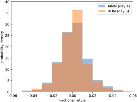
FIGURE 4. Probability densities of the fractional returns for trading MMM on day 4 and XOM on day 5 based on the $p<0.01$ length-5 motif XOM → VZ → BA → MMM → XOM, between Feb 16, 1990 and Mar 8, 2018.

The average fractional returns are 0.0012 for MMM, and 0.0007 for XOM. These are positive, but puny. More importantly, over the roughly 28-year period, we would have traded only $\left(964+477\right)/28=51.5$ times a year based on the motif XOM → VZ → BA → MMM → XOM. A human trader can easily trade many more times, let alone trading algorithms. Therefore, we next check the distribution of fractional returns shown in Figure 5, if we trade on day 4 (60,153 transactions) and day 5 (35,855 transactions) for all $p<0.01$ length-5 motifs. The average fractional return on day 4 is 0.0035, while that on day 5 is 0.0042. While these average fractional returns are higher than those for XOM → VZ → BA → MMM → XOM alone, the distributions shown in Figure 5 give us the wrong impression that trading in these motifs is high-risk and low-return. To put it more accurately, we get such dismal performance only if we choose to trade one random motif a week.

FIGURE 5

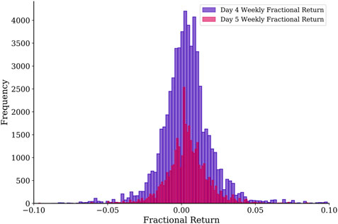
FIGURE 5. Distributions of fractional returns for trading on day 4 and day 5 of $p<0.01$ length-5 motifs in the first cross section of DJI component stocks, comprising (A) GE, (B) CSCO, (C) HD, (D) JPM, (E) MMM, (F) MRK, (G) UTX, (H) BA, (I) VZ, (J) XOM, between Feb 16, 1990 and Mar 8, 2018.

If we trade multiple motifs in the same week, then our prospects would be different. This is because we may fail to profit from some motifs, but still succeed in other motifs. Therefore, we should first average the fractional return over all motifs we trade in a given week, before compiling the histogram of 424 weekly average fractional returns shown in Figure 6. Unlike for the fractional return of individual transactions, when we trade all possible motifs and average the fractional returns over them, we find that we almost never lose money in any week. The average of the average fractional return per week is 0.0035 on day 4 and 0.0042 on day 5, the same as when we average over the distributions of fractional returns. However, since we now know the average fractional return per week is (almost) always positive, we can compound them to get an average fractional return of 0.0077 per week, or an average fractional return of 0.4004 per annum!

FIGURE 6

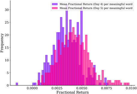
FIGURE 6. Distributions of weekly average fractional returns for trading on day 4 and day 5 of all $p<0.01$ length-5 motifs in the first cross section of DJI component stocks, comprising (A) GE, (B) CSCO, (C) HD, (D) JPM, (E) MMM, (F) MRK, (G) UTX, (H) BA, (I) VZ, (J) XOM, between Feb 16, 1990 and Mar 8, 2018.

Another way to understand this profitability is in terms of $p\left(X_4>0|X_1>0,X_2>0,X_3>0\right)$, which is the conditional probability for a price increase $X_4>0$ to be observed on day 4, given that price increases $X_1>0$, $X_2>0$, $X_3>0$ have been observed on day 1, day 2, and day 3 for a given length-5 motif, and $p\left(X_5>0|X_1>0,X_2>0,X_3>0,X_4>0\right)$, which is the conditional probability for a price increase $X_5>0$ to be observed on day 5, given that price increases $X_1>0$, $X_2>0$, $X_3>0$, $X_4>0$ have been observed on day 1, day 2, day 3, and day 4 for the same length-5 motif. When we plot these conditional probabilities as a violin plot in Figure 7, we see that the conditional probability for day 4 is mostly larger than 0.5. There seems to be no correlation between the strength of this conditional probability and the strength of the stocks as leaders. Finally, we see that the conditional probability for day 5 is significantly larger than 0.5.

FIGURE 7

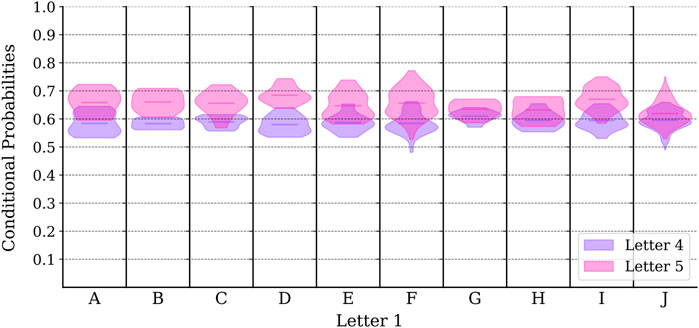
FIGURE 7. Distributions of conditional probabilities for price increases on day 4 and day 5 for all $p<0.01$ length-5 motifs in the first cross section of DJI component stocks, comprising (A) GE, (B) CSCO, (C) HD, (D) JPM, (E) MMM, (F) MRK, (G) UTX, (H) BA, (I) VZ, (J) XOM, between Feb 16, 1990 and Mar 8, 2018. Since we distinguish between strong and weak leaders, in this figure we show the conditional probabilities for motifs with different roots from (A) to (J).

Before we conclude, let us also test the feasibility of our simple trading strategy for the $p<0.01$ length-5 motifs in the first cross section of nine mixed assets, comprising (A) gold, (B) silver, (C) palladium, (D) S&P P 500, (E) Hang Seng, (F) platinum, (G) Dow Jones, (H) Nikkei, and (I) NASDAQ. If we trade one random motif each week, we would have the distributions of fractional returns shown in Figure 8. Based on these distributions, the average fractional return on day 4 (558,752 transactions) is 0.0025, while that on day 5 (318,509 transactions) is 0.0028. However, if we trade all possible motifs each week, we would have the distributions of 3,182 weekly fractional return shown in Figure 9. Just like for the first cross section of DJI stocks, the average weekly fractional returns on day 4 and day 5 are still 0.0025 and 0.0029, but as we can see from Figure 9, the downside risk of getting negative average weekly fractional returns is greatly reduced. As we can see from the violin plot in Figure 10, most of the conditional probabilities on day 5 are larger than their counterparts on day 4. However, only the day-5 conditional probabilities of motifs starting with (E) Hang Seng and (H) Nikkei are significantly larger than 0.5.

FIGURE 8

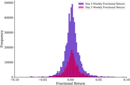
FIGURE 8. Histograms of the fractional returns for day 4 and day 5 trading based on $p<0.01$ length-5 motifs from the first cross section of nine mixed assets, comprising (A) gold, (B) silver, (C) palladium, (D) S&P 500, (E) Hang Seng, (F) platinum, (G) Dow Jones, (H) Nikkei, and (I) NASDAQ, using prices between Apr 2, 1990 and Jan 28, 2018.

FIGURE 9

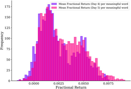
FIGURE 9. Histograms of the weekly average fractional returns for day 4 and day 5 trading based on all $p<0.01$ length-5 motifs from the first cross section of nine mixed assets, comprising (A) gold, (B) silver, (C) palladium, (D) S&P 500, (E) Hang Seng, (F) platinum (G) Dow Jones, (H) Nikkei, and (I) NASDAQ, using prices between Apr 2, 1990 and Jan 28, 2018.

FIGURE 10

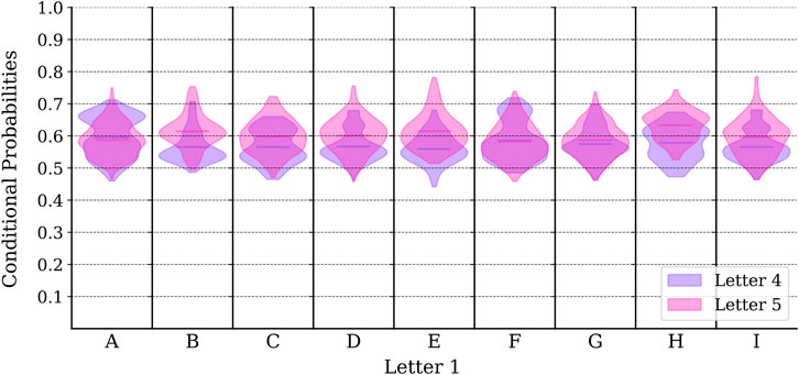
FIGURE 10. Histograms of the conditional probabilities for day 4 and day 5 trading based on all $p<0.01$ length-5 motifs from the first cross section of nine mixed assets, comprising (A) gold, (B) silver, (C) palladium, (D) S&P 500, (E) Hang Seng, (F) platinum, (G) Dow Jones, (H) Nikkei, and (I) NASDAQ, using prices between Apr 2, 1990 and Jan 28, 2018.

We also investigated a second cross section of DJI stocks, as well as a second and third cross sections of mixed assets. The distributions of fractional returns, weekly average fractional returns, and conditional probabilities of these cross sections are shown in Supplementary Figures S8 and S9.

5 Conclusions and Outlook

In this paper, we explained how information processing by self-organized functions in complex systems lead to the existence of recurrent activity sequences or dynamical motifs. In financial markets, which are also complex systems, past and expected information that gets incorporated into prices must therefore be in the form of recurrent sequences. Thus far, technical traders have exploited temporal patterns corresponding to high-order serial correlations of individual instruments, but actionable spatio-temporal patterns (also called dynamical motifs) must also exist. To identify these dynamical motifs ${\text{Σ}}_k={\sigma }_{k,1}\to {\sigma }_{k,2}\to \cdots \to {\sigma }_{k,m_k}$ with $m_k$ spatial cross sections, ${\sigma }_{k,l}=\left(s_{k,l,1},s_{k,l,2},\dots ,s_{k,l,p_{k,l}}\right)$, each of which containing $p_{k,l}$ activities, we first described a procedure for mapping price increases in a spatial cross section of financial instruments to an alphabet, so that price increases in the cross section can be mapped first to a symbolic spatio-temporal sequence, and then unpacked into a collection of temporal sequences represented as simple strings. We then described how statistically significant temporal sequences can be identified by testing the empirical frequencies of these frequencies against a null model obtained by reshuffling the spatio-temporal sequence (or collection of spatio-temporal sequences). Such a null model preserves equal-time spatial cross correlations, but completely destroys any serial correlations. Dynamical motifs that traders can act on are thus temporal sequences that occur more frequently then expected from the null model.

We tested the above procedure on the 30 DJI component stocks, as well as 26 instruments from various asset classes, to find the absence of serial correlations that traders can exploit, if they are traded individually. We then tested the procedure on two pairs of instruments, to find two length-4 dynamical motifs for (HD, TRV) that are statistically significant at the $p<0.01$ level, and one length-2 dynamical motif for (platinum, USD-EUR) that is statistically significant at the $p<0.01$ level. After testing the procedure next on a cross section of five DJI component stocks, and finding 35 dynamical motifs (29 of which are length-5) that are statistically significant at the $p<0.01$ level, we proceeded to identify dynamical motifs in five cross sections containing eight to ten instruments. For a cross section of 10 DJI component stocks and a cross section of nine mixed assets, we reported in detail the 672 and 9,145 dynamical motifs that are statistically significant at the $p<0.01$ level, how to identify leaders and followers, and more importantly, how to visualize these in the form of tree diagrams with different roots. Finally, we checked using our historical data whether these dynamical motifs can be traded feasibly, by targeting the price increases expected on day 4 and day 5 in length-5 motifs. We showed that if we trade only a single dynamical motif, the downside risk is appreciable, even though the expected fractional return is positive. While the expected fractional return is not greatly improved by trading all $p<0.01$ length-5 motifs, we found that the downside risk is greatly reduced. This is true for the 10-DJI-component-stock cross section, as well as for the 9-mixed-assets cross section. For the 10-DJI-component-stock cross section with 616 $p<0.01$ length-5 motifs, downside risk was practically non-existent, and an expected fractional return of 0.0077 per week, or equivalently 0.4004 per annum could be achieved.

In this study, we identified dynamical motifs consisting of price increases over five consecutive days from daily prices. For 616 length-5 motifs in the cross section of 10 DJI component stocks, we could execute 96,000 trades over 28 years, or about 3,400 trades per year. For 9,145 length-5 motifs in the cross section of nine mixed assets, we could execute about 877,300 trades, or about 31,300 trades per year. To get better returns, a trader would want to trade more frequently. This can be done by going to higher-frequency data, and use the high-frequency motifs identified for trading. We do not know how well such a strategy will perform, but imagine it doing better, since in high-frequency data, autocorrelations and cross correlations do not have time to die out, and therefore motifs would become easier to identify, and are also statistically more significant. In this paper, we also mapped all price increases in an instrument to a single letter. If we do not have many instruments, it is possible (and perhaps desirable) to use two letters per instrument, so that one would represent a small increase, while the other would represent a large increase. Alternatively, we can map the price increases in an instrument to more than one instance of the letter. For example, an increase of 0–1% can be mapped to A, an increase of 1–2% to AA, and an increase of 2–5% to AAA. Traders can then choose to act only if a large price increase is expected. Other variations are also possible.

As a final caveat, let us say that like for purely temporal patterns of single instruments, the profitabilities of spatio-temporal patterns containing multiple instruments are also expected to be short-lived, because once a spatio-temporal pattern becomes dominant it can be exploited by other spatio-temporal patterns. In Figure 11 we show the frequencies of two length-5 motifs (at the $p<0.01$ of statistical significance) over the period 1990 to 2018. In general, these frequencies are low, so for the most part it is difficult to tell visually whether they occurred uniformly over the period, or their occurrences were concentrated over certain subperiods. However, the frequency spike of MMM → CSCO → HD → CSCO → CSCO in 2016 will surely not be the product of a uniform probability that produced the frequencies in other years. Even though this has not happened in our data sets, we must be prepared for the eventuality of temporal motifs losing their statistical significance. Therefore, as we trade the significant sequences, we must at the same time be mining for new significant sequences. Once these latter sequences are discovered, they should be added to the trading pool, but we must also develop the criterion for discarding sequences that are no longer significant. This must be done in a way that maximizes the lifetime returns from such sequences, weighted against the potential for losses at the end of their usable lifetimes.

FIGURE 11

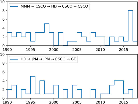
FIGURE 11. The number of times two length-5 motifs ((top) MMM → CSCO → HD → CSCO → CSCO, and (bottom) HD → JPM → JPM → CSCO → GE) in the cross section of five DJI component stocks (A) GE, (B) CSCO, (C) HD, (D) JPM, (E) MMM, appear for each year between Feb 16, 1990 and Mar 8, 2018.

Data Availability Statement

The datasets presented in this study can be found in online repositories. The names of the repository/repositories and accession number(s) can be found in the article/Supplementary Material.

Author Contributions

SC conceived the study, wrote some of the Python programs, and wrote the manuscript. YWL, YYL, JL, JT, and XT downloaded the data sets and wrote the rest of the Python programs. All authors analyzed the results and reviewed the manuscript.

Conflict of Interest

The authors declare that the research was conducted in the absence of any commercial or financial relationships that could be construed as a potential conflict of interest.

Acknowledgments

YWL, YYL, JL, JT, and XT thank the Singapore Ministry of Education Science Mentorship Program for the opportunity to participate in this study.

Supplementary Material

The Supplementary Material for this article can be found online at: https://www.frontiersin.org/articles/10.3389/fams.2021.641595/full#supplementary-material.

References

1. Fama, EF. Efficient Capital Markets: A Review of Theory and Empirical Work. J Finance (1970). 25:383–417. doi:10.2307/2325486

CrossRef Full Text | Google Scholar

2. Brown, DP, and Jennings, RH. On Technical Analysis. Rev Financ Stud (1989). 2:527–51. doi:10.1093/rfs/2.4.527

CrossRef Full Text | Google Scholar

3. Park, CH, and Irwin, SH. What Do We Know About the Profitability of Technical Analysis? J Econ Surv (2007). 21:786–826. doi:10.1111/j.1467-6419.2007.00519.x

CrossRef Full Text | Google Scholar

4. Nazário, RT, e Silva, JL, Sobreiro, VA, and Kimura, H. A Literature Review of Technical Analysis on Stock Markets. Q Rev Econ Finance (2017). 66:115–26. doi:10.1016/j.qref.2017.01.014

CrossRef Full Text | Google Scholar

5. Lukac, LP, Brorsen, BW, and Irwin, SH. A Test of Futures Market Disequilibrium Using Twelve Different Technical Trading Systems. Appl Econ (1988). 20:623–39. doi:10.1080/00036848800000113

CrossRef Full Text | Google Scholar

6. Brock, W, Lakonishok, J, and LeBaron, B. Simple Technical Trading Rules and the Stochastic Properties of Stock Returns. J Finance (1992). 47:1731–64. doi:10.2307/2328994

CrossRef Full Text | Google Scholar

7. Levich, RM, and Thomas, LR. The Significance of Technical Trading-Rule Profits in the Foreign Exchange Market: A Bootstrap Approach. J Int Money Finance (1993). 12:451–74. doi:10.1016/0261-5606(93)90034-9

CrossRef Full Text | Google Scholar

8. Parisi, F, and Vasquez, A. Simple Technical Trading Rules of Stock Returns: Evidence From 1987 to 1998 in Chile. Emerg Mark Rev (2000). 1:152–64. doi:10.1016/S1566-0141(00)00006-6

CrossRef Full Text | Google Scholar

9. Kwon, KY, and Kish, RJ. Technical Trading Strategies and Return Predictability: NYSE. Appl Financ Econ (2002). 12:639–53. doi:10.1080/09603100010016139

CrossRef Full Text | Google Scholar

10. Ready, MJ. Profits From Technical Trading Rules. Financ Manage (2002). 31:43–61. doi:10.2307/3666314

CrossRef Full Text | Google Scholar

11. Bajgrowicz, P, and Scaillet, O. Technical Trading Revisited: False Discoveries, Persistence Tests, and Transaction Costs. J Financ Econ (2012). 106:473–91. doi:10.1016/j.jfineco.2012.06.001

CrossRef Full Text | Google Scholar

12. Fang, J, Jacobsen, B, and Qin, Y. Predictability of the Simple Technical Trading Rules: An Out-of-Sample Test. Rev Financ Econ (2014). 23:30–45. doi:10.1016/j.rfe.2013.05.004

CrossRef Full Text | Google Scholar

13. Taylor, N. The Rise and Fall of Technical Trading Rule Success. J Bank Finance (2014). 40:286–302. doi:10.1016/j.jbankfin.2013.12.004

CrossRef Full Text | Google Scholar

14. Ackermann, C, McEnally, R, and Ravenscraft, D. The Performance of Hedge Funds: Risk, Return, and Incentives. J Finance (1999). 54:833–74. doi:10.1111/0022-1082.00129

CrossRef Full Text | Google Scholar

15. Liang, B. On the Performance of Hedge Funds. Financ Anal J (1999). 55:72–85. doi:10.2139/SSRN.89490

CrossRef Full Text | Google Scholar

16. Fung, W, Hsieh, DA, Naik, NY, and Ramadorai, T. Hedge Funds: Performance, Risk, and Capital Formation. J Finance (2008). 63:1777–803. doi:10.1111/j.1540-6261.2008.01374.x

CrossRef Full Text | Google Scholar

17. Allen, F, and Karjalainen, R. Using Genetic Algorithms to Find Technical Trading Rules. J Financ Econ (1999). 51:245–71. doi:10.1016/S0304-405X(98)00052-X

Google Scholar

18. Fernández-Rodríguez, F, González-Martel, C, and Sosvilla-Rivero, S. On the Profitability of Technical Trading Rules Based on Artificial Neural Networks: Evidence from the Madrid Stock Market. Econ Lett (2000). 69:89–94. doi:10.1016/S0165-1765(00)00270-6

CrossRef Full Text | Google Scholar

19. Kimoto, T, Asakawa, K, Yoda, M, and Takeoka, M. Stock Market Prediction System with Modular Neural Networks. In: Proceedings of the 1990 International Joint Conference on Neural Networks (IJCNN 1990); 1990 June 17–21; San Diego, CA. New York, NY: IEEE. (2009). p. 1–6.

Google Scholar

20. Zhang, Y, and Wu, L. Stock Market Prediction of S&P 500 via Combination of Improved BCO Approach and BP Neural Network. Expert Syst Appl (2009). 36:8849–54. doi:10.1016/j.eswa.2008.11.028

CrossRef Full Text | Google Scholar

21. Guresen, E, Kayakutlu, G, and Daim, TU. Using Artificial Neural Network Models in Stock Market Index Prediction. Expert Syst Appl (2011). 38:10389–97. doi:10.1016/j.eswa.2011.02.068

CrossRef Full Text | Google Scholar

22. Wise, J, Roush, R, and Fowler, S. Concepts of Biology. Scotts Valley, CA: CreateSpace Independent Publishing Platform (2013).

23. Tymoczko, JL, Berg, JM, Stryer, L, and Gatto, G. Biochemistry: A Short Course. Austin, TX: Macmillan Learning (2019).

24. Spiegel, S, Gaebler, J, Lommatzsch, A, De Luca, E, and Albayrak, S. Pattern Recognition and Classification for Multivariate Time Series. In: Proceedings of the Fifth International Workshop on Knowledge Discovery from Sensor Data; August 21, 2011, San Diego, CA. New York, NY: ACM (2011). p. 34–42.

Google Scholar

25. Fontes, CH, and Pereira, O. Pattern Recognition in Multivariate Time Series – A Case Study Applied to Fault Detection in a Gas Turbine. Eng Appl Artif Intell (2016). 49:10–8. doi:10.1016/j.engappai.2015.11.005

CrossRef Full Text | Google Scholar

26. Zhang, YQ, Li, X, Xu, J, and Vasilakos, AV. Human Interactive Patterns in Temporal Networks. IEEE Trans Syst Man Cybern Syst (2015). 45:214–22. doi:10.1109/TSMC.2014.2360505

Google Scholar

27. Hulovatyy, Y, Chen, H, and Milenković, T. Exploring the Structure and Function of Temporal Networks With Dynamic Graphlets. Bioinformatics (2015). 31:i171–80. doi:10.1093/bioinformatics/btv227

PubMed Abstract | CrossRef Full Text | Google Scholar

28. Xuan, Q, Fang, H, Fu, C, and Filkov, V. Temporal Motifs Reveal Collaboration Patterns in Online Task-Oriented Networks. Phys Rev E (2015). 91:052813. doi:10.1103/PhysRevE.91.052813

PubMed Abstract | CrossRef Full Text | Google Scholar

29. Paranjape, A, Benson, AR, and Leskovec, J. Motifs in Temporal Networks. In: Proceedings of the Tenth ACM International Conference on Web Search and Data Mining (WSDM 2017); 2017 Feb 6–10; Cambridge, UK. New York, NY: ACM (2017). p. 601–10.

Google Scholar

30. Liu, P, Benson, AR, and Charikar, M. Sampling Methods for Counting Temporal Motifs. In: Proceedings of the Twelfth ACM International Conference on Web Search and Data Mining; 2019 Feb 11–15; Melbourne, Australia. New York, NY: ACM (2019). p. 294–302.

Google Scholar

31. Goh, WP, Luke, KK, and Cheong, SA. Functional Shortcuts in Language Co-Occurrence Networks. PLoS ONE (2018). 13:0203025. doi:10.1371/Fjournal.pone.0203025

PubMed Abstract | CrossRef Full Text | Google Scholar

32. Goh, WP, Kwek, D, Hogan, D, and Cheong, SA. Complex Network Analysis of Teaching Practices. Eur Phys J Data Sci (2014). 3:34. doi:10.1140/epjds/s13688-014-0034-9

CrossRef Full Text | Google Scholar

33. Kelly, JL. A New Interpretation of Information Rate. In: LC McClean, EO Thorp, and WT Ziemba, editors. The Kelly Capital Growth Investment Criterion. Singapore: World Scientific (2011). p. 25–34.

CrossRef Full Text | Google Scholar

34. Milo, R, Shen-Orr, S, Itzkovitz, S, Kashtan, N, Chklovskii, D, and Alon, U. Network Motifs: Simple Building Blocks of Complex Networks. Science (2002). 298:824–7. doi:10.1126/science.298.5594.824

PubMed Abstract | CrossRef Full Text | Google Scholar

35. Shen-Orr, SS, Milo, R, Mangan, S, and Alon, U. Network Motifs in the Transcriptional Regulation Network of Escherichia coli. Nat Genet (2002). 31:64–8. doi:10.1038/ng881

PubMed Abstract | CrossRef Full Text | Google Scholar

36. Wernicke, S, and Rasche, F. FANMOD: A Tool for Fast Network Motif Detection. Bioinformatics (2006). 22:1152–3. doi:10.1093/bioinformatics/btl038

PubMed Abstract | CrossRef Full Text | Google Scholar

37. Kovanen, L, Karsai, M, Kaski, K, Kertész, J, and Saramäki, J. Temporal Motifs in Time-Dependent Networks. J Stat Mech Theor Exp. (2011). P11005. doi:10.1088/1742-5468/2011/11/P11005

CrossRef Full Text | Google Scholar

38. Kovanen, L, Kaski, K, Kertész, J, and Saramäki, J. Temporal Motifs Reveal Homophily, Gender-Specific Patterns, and Group Talk in Call Sequences. Proc Natl Acad Sci U S A (2013). 110:18070–5. doi:10.1073/pnas.1307941110

PubMed Abstract | CrossRef Full Text | Google Scholar

39. Dunn, OJ. Multiple Comparisons Among Means. J Am Stat Assoc (1961). 56:52–64. doi:10.1080/01621459.1961.10482090

CrossRef Full Text | Google Scholar

40. Šidák, Z. Rectangular Confidence Regions for the Means of Multivariate Normal Distributions. J Am Stat Assoc (1967). 62:626–33. doi:10.1080/01621459.1967.10482935

CrossRef Full Text | Google Scholar

41. Chakraborti, A, Toke, IM, Patriarca, M, and Abergel, F. Econophysics Review: I. Empirical Facts. Quant Finance (2011). 11:991–1012. doi:10.1080/14697688.2010.539248

CrossRef Full Text | Google Scholar

42. Moore, GH. Gold Prices and a Leading Index of Inflation. Challenge (1990). 33:52. doi:10.1016/S0148-6195(97)00034-9

CrossRef Full Text | Google Scholar

43. Mahdavi, S, and Zhou, S. Gold and Commodity Prices as Leading Indicators of Inflation: Tests of Long-Run Relationship and Predictive Performance. J Econ Bus (1997). 49:475–89. doi:10.1016/S0148-6195(97)00034-9

CrossRef Full Text | Google Scholar

44. Vodenska, I, Aoyama, H, Fujiwara, Y, Iyetomi, H, and Arai, Y. Interdependencies and Causalities in Coupled Financial Networks. PloS One (2016). 11:0150994. doi:10.1371/journal.pone.0150994

PubMed Abstract | CrossRef Full Text | Google Scholar

45. Kato, K. Weekly Patterns in Japanese Stock Returns. Manage Sci (1990). 36:1031–43. doi:10.1287/mnsc.36.9.1031

CrossRef Full Text | Google Scholar

46. Becker, KG, Finnerty, JE, and Tucker, AL. The Intraday Interdependence Structure Between US and Japanese Equity Markets. J Financ Res (1992). 15:27–37. doi:10.1111/j.1475-6803.1992.tb00784.x

CrossRef Full Text | Google Scholar

47. Pan, MS, and Hsueh, LP. Transmission of Stock Returns and Volatility Between the US and Japan: Evidence from the Stock Index Futures Markets. Asia-Pacific Finan Markets (1998). 5:211–25. doi:10.1023/A:1010000606092

CrossRef Full Text | Google Scholar