1 Introduction
Since it has been realized that many signals admit a sparse representation in some frames, the question arose whether or not such signals can be recovered from less samples than the dimension of the domain by utilizing the low dimensional structure of the signal. The question was already answered positively in the beginning of the millennium [1, 2]. By now there are multiple different decoders to recover a sparse signal from noisy measurements with robust recovery guarantees. Most of them however rely on some form of tuning, depending on either the signal or the noise.
The basis pursuit denoising requires an upper bound on the norm of the noise ([3], Theorem 4.22), the least shrinkage and selection operator an estimate on the -norm of the signal ([4], Theorem 11.1) and the Lagrangian version of least shrinkage and selection operator allegedly needs to be tuned to the order of the the noise level ([4], Theorem 11.1). The expander iterative hard thresholding needs the sparsity of the signal or an estimate of the order of the expansion property ([3], Theorem 13.15). The order of the expansion property can be calculated from the measurement matrix, however there is no polynomial time method known to do this. Variants of these methods have similar drawbacks. The non-negative basis pursuit denoising requires the same tuning parameter as the basis pursuit denoising [5]. Other thresholding based decoders like sparse matching pursuit and expander matching pursuit have the same limitations as the expander iterative hard thresholding [6].
If these side information is not known a priori, many decoders yield either no recovery guarantees or, in their imperfectly tuned versions, yield sub-optimal estimation errors ([3], Theorem 11.12). Even though the problem of sparse recovery from under-sampled measurements has been answered long ago, finding tuning free decoders that achieve robust recovery guarantees is still a topic of interest.
The most prominent achievement for that is the non-negative least squares (NNLS) [7–11]. It is completely tuning free [12] and in [13, 14] it was proven that it achieves robust recovery guarantees if the measurement matrix consists of independent biased sub-Gaussian random variables.
1.1 Our Contribution
We will replace the least squares in the NNLS with an arbitrary norm and obtain the non-negative least residual (NNLR). We use the methods of [13] to prove recovery guarantees under similar conditions as the NNLS. In particular, we consider the case where we minimize the -norm of the residual (NNLAD) and give a recovery guarantee if the measurement matrix is a random walk matrix of a uniformly at random drawn D-left regular bipartite graph.
In general, our results state that if the criterion is fulfilled, the basis pursuit denoising can be replaced by the tuning-less NNLR for non-negative signals. Note that the M+criterion can be fulfilled by adding only one explicitly chosen measurement if that is possible in the application. Thus, in practice the NNLR does not require more measurements than the BPDN to recover sparse signals. While biased sub-Gaussian measurement matrices rely on a probabilistic argument to verify that such a measurement is present, random walk matrices of left regular graphs naturally have such a measurement. The tuning-less nature gives the NNLR an advantage over other decoders if the noise power can not be estimated, which is for instance the case when we have multiplicative noise or the measurements are Poisson distributed. Note that Laplacian distributed noise or the existence of outliers also favors an regression approach over an regression approach and thus motivate to use the NNLAD over the NNLS.
Further, the sparse structure of left regular graphs can reduce the encoding and decoding time to a fraction. Using [15] we can solve the NNLAD with a first order method of a single optimization problem with a sparse measurement matrix. Other state of the art decoders often use non-convex optimization, computationally complex projections or need to solve multiple different optimization problems. For instance, to solve the basis pursuit denoising given a tuning parameter a common approach is to solve a sequence of -constrained least residual1 problems to approximate where the Pareto curve attains the value of the tuning parameter of basis pursuit denoising [16]. Cross-validation techniques suffer from similar issues [17].
1.2 Relations to Other Works
We build on the theory of [13] that uses the null space property and the criterion. These methods have also been used in [12, 14]. To the best of the authors knowledge the criterion has not been used with an null space property before. Other works have used adjacency matrices of graphs as measurements matrices including [6, 18–21]. The works [18, 19] did not consider noisy observations. The decoder in [20] is the basis pursuit denoising and thus requires tuning depending on the noise power. [21] proposes two decoders for non-negative signals. The first is the non-negative basis pursuit which could be extended to the non-negative basis pursuit denoising. However, this again needs a tuning parameter depending on the noise power. The second decoder, the Reverse Expansion Recovery algorithm, requires the order of the expansion property, which is not known to be calculatable in a polynomial time. The survey [6] contains multiple decoders including the basis pursuit, which again needs tuning depending on the noise power for robustness, the expander matching pursuit and the sparse matching pursuit, which need the order of the expansion property. Further, [5] considered sparse regression of non-negative signals and also used the non-negative basis pursuit denoising as decoder, which again needs tuning dependent on the noise power. To the best of the authors knowledge, this is the first work that considers tuning-less sparse recovery for random walk matrices of left regular bipartite graphs. The NNLAD has been considered in [22] with a structured sparsity model without the use of the criterion.
2 Preliminaries
For we denote the set of integers from 1 to K by . For a set we denote the number of elements in T by . Vectors are denoted by lower case bold face symbols, while its corresponding components are denoted by lower case italic letters. Matrices are denoted by upper case bold face symbols, while its corresponding components are denoted by upper case italic letters. For we denote its -norms by . Given we denote its operator norm as operator from to by . By we denote the non-negative orthant. Given a closed convex set , we denote the projection onto C, i.e., the unique minimizer of , by . For a vector and a set , denotes the vector in , whose nth component is if and 0 else. Given we will often need sets with and we abbreviate this by if no confusion is possible.
Given a measurement matrix a decoder is any map . We refer to as signal. If , we say the signal is non-negative and write shortly . If additionally for all , we write . An input of a decoder, i.e., any , is refered to as observation. We allow all possible inputs of the decoder as observation, since in general the transmitted codeword is disturbed by some noise. Thus, given a signal and an observation we call the noise. A signal is called S-sparse if . We denote the set of S-sparse vectors by
Given some the compressibility of a signal can be measured by .Given N and S, the general non-negative compressed sensing task is to find a measurement matrix and a decoder with M as small as possible such that the following holds true: There exists a and a continuous function with such that
holds true. This will ensure that if we can control the compressibility and the noise, we can also control the estimation error and in particular decode every noiseless observation of S-sparse signals exactly.
3 Main Results
Given a measurement matrix and a norm on we define the decoder as follows: Given set (y) as any minimizer of
We call this problem non-negative least residual (NNLR). In particular, for this problem is called non-negative least absolute deviation (NNLAD) and for this problem is known as the non-negative least squares (NNLS) studied in [13]. In fact, we can translate the proof techniques fairly simple. We just need to introduce the dual norm.
Definition 3.1. Let be a norm on . The norm on defined by
is called dual norm to .
Note that the dual norm is actually a norm. To obtain a recovery guarantee for NNLR we have certain requirements on the measurement matrix . We use a null space property.
Definition 3.2. Let , and be any norm on . Further let . Suppose there exists constants and such that
Then, we say has the -robust null space property of order S with respect to or in short has the -RNSP of order S with respect to with constants ρ and τ. ρ is called stableness constant and τ is called robustness constant.
Note that smaller stableness constants increase the reliability of recovery if many, small, non-zero components are present, while smaller robustness constants increase the reliability if the measurements are noisy. In order to make use of the non-negativity of the signal, we need to be biased in a certain way. In [13] this bias was guaranteed with the criterion.
Definition 3.3. Let . Suppose there exists such that . Then we say obeys the the criterion with vector and constant .
Note that κ is actually a condition number of the matrix with diagonal and 0 else. Condition number numbers are frequently used in error bounds of numerical linear algebra. The general recovery guarantee is the following and similar results have been obtained in the matrix case in [23].
Theorem 3.4 (NNLR Recovery Guarantee). Let , and be any norm on with dual norm . Further, suppose that obeys
a) the -RNSP of order S with respect to with constants ρ and τ and
b) the criterion with vector and constant κ.
If , the following recovery guarantee holds true: For all and any minimizer of
obeys the bound
If , this bound can be improved to
Proof The proof can be found in Subsection 6.1.
Given a matrix with -RNSP we can add a row of ones (or a row consisting of one minus the column sums of the matrix) to fulfill the criterion with the optimal . Certain random measurement matrices guarantee uniform bounds on κ for fixed vectors . In ([13], Theorem 12) it was proven that if are all i.i.d. Bernoulli random variables, has criterion with and with high probability. This is problematic, since if , it might happen that is not fulfilled anymore. Since the stableness constant as a function of is monotonically increasing, the condition might only hold if . If that is the case, there are vectors that are being recovered by basis pursuit denoising but not by NNLS! This is for instance the case for the matrix , which has -robust null space property of order 1 with stableness constant and criterion with for any possible choice of . In particular, the vector is not necessarily being recovered by the NNLAD and the NNLS.
Hence, it is crucial that the vector is chosen to minimize κ and ideally obeys the optimal . This motivates us to use random walk matrices of regular graphs since they obey exactly this.
Definition 3.5. Let and . For the set
is called the set of right vertices connected to the set of left vertices T. If
then is called a random walk matrix of a D-left regular bipartite graph. We also say short that is a D-LRBG. If additionally there exists a such that
holds true, then is called a random walk matrix of a -lossless expander.
Note that we have made a slight abuse of notation. The term D-LRBG as a short form for D-left regular bipartite graph refers in our case to the random walk matrix but not the graph itself. We omit this minor technical differentiation, for the sake of shortening the frequently used term random walk matrix of a D-left regular bipartite graph. Lossless expanders are bipartite graphs that have a low number of edges but are still highly connected, see for instance ([24], Chapter 4). As a consequence their random walk matrices have good properties for compressed sensing. It is well known that random walk matrices of a -lossless expanders obey the -RNSP of order S with respect to , see ([3], Theorem 13.11). The dual norm of is the norm and the criterion is easily fulfilled, since the columns sum up to one. From Theorem 3.4 we can thus draw the following corollary.
Corollary 3.6 (Lossless Expander Recovery Guarantee). Let , . If is a random walk matrix of a -lossless expander, then the following recovery guarantee holds true: For all and any minimizer of
obeys the bound
Proof By ([3], Theorem 13.11) has -RNSP with respect to with constants and . The dual norm of the norm is . If we set , we get
Hence, has the criterion with vector and constant and the condition is immediately fulfilled. We obtain and . Applying Theorem 3.4 with improved bound for and these values yields
If we additionally substitute the values for ρ and τ we get
This finishes the proof.
Note that ([3], Theorem 13.11) is an adaption of ([20], Lemma 11) to account for robustness and skips proving the restricted isometry property. If and , a uniformly at random drawn D-LRBG is a random walk matrix of a -lossless expander with a high probability[ [3], Theorem 13.7]. Thus, recovery with the NNLAD is possible in the optimal regime .
3.2 On the Robustness Bound for Lossless Expanders
If is a random walk matrix of a -lossless expander with , then we can also draw a recovery guarantee for the NNLS. By ([3], Theorem 13.11) has -RNSP with respect to with constants and and hence also -RNSP with respect to with constants and . Similar to the proof of Corollary 3.6 we can use Theorem 3.4 to deduce that any minimizer of
obeys the bound
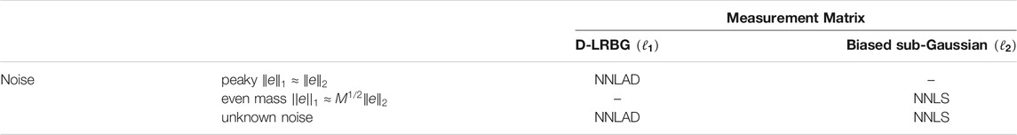
If the measurement error is a constant vector, i.e., , then . In this case the error bound of the NNLS is just as good as the error bound of the NNLAD. However, if is a standard unit vector, then . In this case the error bound of the NNLS is significantly worse than the error bound of the NNLAD. Thus, the NNLAD performs better under peaky noise, while the NNLS and NNLAD are tied under noise with evenly distributed mass. We will verify this numerically in Subsection 5.1. One can draw a complementary result for matrices with biased sub-Gaussian entries, which obey the -RNSP with respect to and the criterion in the optimal regime [13]. Table 1 states the methods, which have an advantage over the other in each scenario.
4 Non-Negative Least Absolute Deviation Using a Proximal Point Method
In this section we assume that with some . If , the NNLR can be recast as a linear program by introducing some slack variables. For an arbitrary p the NNLR is a convex optimization problem and the objective function has a simple and globally bounded subdifferential. Thus, the NNLR can directly be solved with a projective subgradient method using a problem independent step size. Such subgradient methods achieve only a convergence rate of toward the optimal objective value ([25], Section 3.2.3), where k is the number of iterations performed. In the case that the norm is the -norm, we can transfer the problem into a differentiable version, i.e. the NNLS
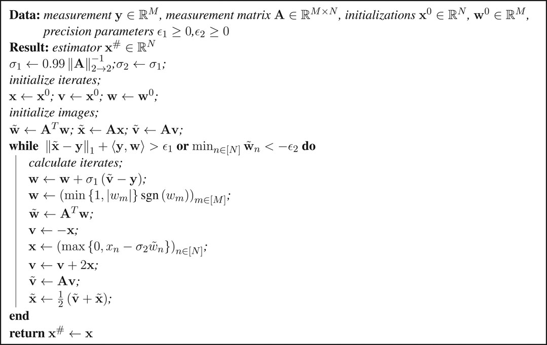
Since the gradient of such an objective is Lipschitz, this problem can be solved by a projected gradient method with constant step size, which achieves a convergence rate of toward the optimal objective value [26, 27]. However this does not generalize to the -norm. The proximal point method proposed in [15] can solve the case of the -norm with a convergence rate toward the optimal objective value. Please refer to Algorithm 1.
Algorithm 1 is a primal-dual algorithm. Within the loop, lines 7, 8, 1 and 2 calculate the proximal point operator of the Fenchel conjugate of to update the dual problem, lines 3 and 5 update the primal problem, and lines 4 and 6 perform a momentum step to accelerate convergence. Further, line 8 sets to and avoids a third matrix vector multiplication. Note that and can be replaced by any values that satisfy . The calculation of and might be a bottle neck for the computational complexity of the algorithm. If one wants to solve multiple problems with the same matrix, and should only be calculated once and not in each run of the algorithm. For any the following convergence guarantee can be deduced from ([15], Theorem 1). Let and be the values of and at the end of the kth iteration of the while loop of Algorithm 1. Then, the following statements hold true:
(1) The iterates converge: The sequence converges to a minimizer of .
(2) The iterates are feasible: We have and for all .
(3) There is a stopping criteria for the iterates: and . In particular, if and , then is a minimizer of .
(5) The averages obey the convergence rate toward the optimal objective value: , where is a minimizer of .
The formal version and proof can be found in [28]. Note that this yields a convergence guarantee for both the iterates and averages, but the convergence rate is only guaranteed for the averages. Algorithm 1 is optimized in the sense that it uses the least possible number of matrix vector multiplications per iteration, since these govern the computational complexity.
Remark 4.1. Let be D-LRBG. Each iteration of Algorithm 1 requires at most floating point operations and assignments.
4.1 Iterates or Averages
The question arises whether or not it is better to estimate with averages or iterates. Numerical testing suggest that the iterates reach tolerance thresholds significantly faster than the averages. We can only give a heuristically explanation for this phenomenon. The stopping criteria of the iterates yields . In practice we observe that for all sufficiently large k. However, yields . This monotonicity promotes the converges of the iterates and gives a clue why the iterates seem to converge better in practice. See Figures 5, 6.
4.2 On the Convergence Rate
As stated the NNLS achieves the convergence rate [27] while the NNLAD only achieves the convergence rate of toward to optimal objective value. However, this should not be considered as weaker, since the objective function of the NNLS is the square of a norm. If are the iterates of the NNLS implementation of [27], algebraic manipulation yields
Thus, the -norm of the residual of the NNLS iterates only decays in the same order as the -norm of the residual of the NNLAD averages.
5 Numerical Experiments and Applications
In the first part of this section we will compare NNLAD with several state of the art recovery methods in terms of achieved sparsity levels and decoding time. For , we denote , and .
5.1 Properties of the Non-Negative Least Absolute Deviation Optimizer
We recall that the goal is to recover from the noisy linear measurements . To investigate properties of the minimizers of NNLAD we compare it to the minimizers of the well studied problems basis pursuit (BP), optimally tuned basis pursuit denoising (BPDN), optimally tuned -constrained least residual (CLR) and the NNLS, which are given by
The NNLAD is designed to recover non-negative signals in general and, as we will see, it is able to recover sparse non-negative signals comparable well to the CLR and BPDN with optimal tuning which are particularly designed for this task. Further, we compare the NNLAD to the expander iterative hard thresholding (EIHT). The EIHT is calculated by stopping the following sequence after a suitable stopping criteria is met:
where is the median of and is a hard thresholding operator, i.e., some minimizer of . There is a whole class of thresholding based decoders for lossless expanders, which all need either the sparsity of the signal or the order of the expansion property as tuning parameter. We choose the EIHT as a represent of this class, since the cluster points of its sequence have robust recovery guarantees ([3], Theorem 13.5). By convex decoders we refer to BPDN, BP, CLR, NNLAD, and NNLS. We choose the optimal tuning for the BPDN and for the CLR. The optimally tuned BPDN and CLR are representing a best case benchmark. In ([29], Figure 1.1) it was noticed that tuning the BPDN with often leads to worse estimation errors than tuning with for . Thus, BP is a version of BPDN with no prior knowledge about the noise and represents a worst case benchmark. At fist we investigate the properties of the estimators. In order to mitigate effects from different implementations we solve all optimization problems with the CVX package of Matlab [30, 31]. For a given we will do the following experiment multiple times:
Experiment 1
1. Generate a measurement matrix uniformly at random among all D-LRBG.
2. Generate a signal uniformly at random from .
3. Generate a noise uniformly at random from .
4. Define the observation .
5. For each decoder calculate an estimator and collect the relative estimation error .
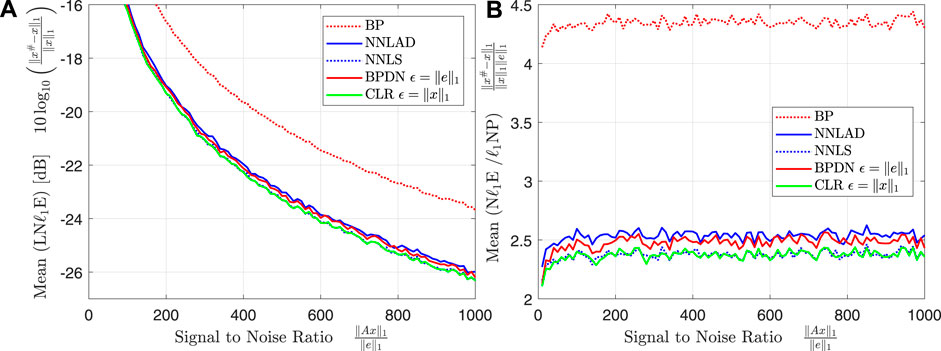
In this experiment we have and since is a D-LRBG and , we further have . Note that for and we obtain two different noise distributions. If is uniformly distributed on , then the absolute value of each component is a random variable with density for . Thus, . By testing one can observe a concentration around this expected value, in particular that with a high probability. If is uniformly distributed on , then . Thus, these two noise distributions each represent randomly drawn noise vectors obeying one norm equivalence asymptotically tightly up to a constant. From Eqs 1,2 we expect that the NNLS has roughly the same estimation errors as the NNLAD for , i.e. the evenly distributed noise, and significantly worse estimation errors for , i.e., the peaky noise.
5.1.1 Quality of the Estimation Error for Varying Sparsity
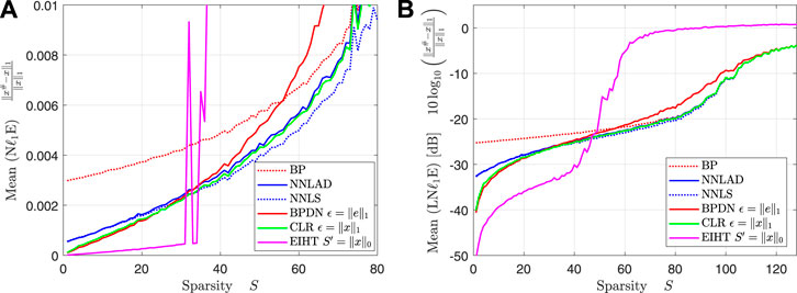
We fix the constants , , , , and vary the sparsity level . For each S we repeat Experiment 1 100 times. We plot the mean of the relative -estimation error and the mean of the logarithmic relative -estimation error, i.e.,
over the sparsity. The result can be found in Figures 1A,B.
For the estimation error of the EIHT randomly peaks high. We deduce that the EIHT fails to recover the signal reliably for , while the NNLAD and other convex decoders succeed. This is not surprising, since by ([3], Theorem 13.15) the EIHT obeys a robust recovery guartanee for S-sparse signals, whenever is the random wak matrix of a -lossless expander with . This is significantly stronger than the -lossless expander property with required for a null space property. It might also be that the null space property is more likely than the lossless expansion property similar to the gap between -restricted isometry property and null space property [32]. However, if the EIHT recovers a signal, it recovers it significantly better than any convex method. This might be the case, since the originally generated signal is indeed from , which is being enforced by the hard thresholding of the EIHT, but not by the convex decoders. This suggests that it might be useful to consider using thresholding on the output of any convex decoder to increase the accuracy if the orignal signal is indeed sparse and not only compressible. For the remainder of this subsection we focus on convex decoders.
Contrary to our expectation the BPDN achieves worse estimation errors than all other convex decoders for , even worse than the BP. The authors have no explanation for this phenomenon. Apart from that we observe that the CLR and BP indeed perform as respectively best and worst case benchmark. However, the difference between BP and CLR becomes rather small for high S. We deduce that tuning becomes less important near the optimal sampling rate.
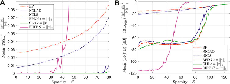
The NNLAD, NNLS and CLR achieve roughly the same estimation errors. However, note that the BPDN and CLR are optimally tuned using unknown prior information unlike the NNLAD and NNLS. As expected the NNLS performs roughly the same as the NNLAD, see Table 1. However, this is the result of the noise distribution for . We repeat Experiment 1 with the same constants, but , i.e., is a unit vector scaled by . We plot the mean of the relative -estimation error and the mean of the logarithmic relative -estimation error over the sparsity. The result can be found in Figures 2A,B.
We want to note that similarly to Figure 1A the EIHT works only unreliably for . Even though the mean of the logarithmic relative -estimation error of NNLS is worse than the one of EIHT for , the NNLS does not fail but only approximates with a weak error bound. As the theory suggests, the NNLS performs significantly worse than the NNLAD, see Table 1. It is worth to mention, that the estimaton errors of NNLS seem to be bounded by the estimation errors of BP. This suggests that obeys a quotient property, that bounds the estimation error of any instance optimal decoder, see ([3], Lemma 11.15).
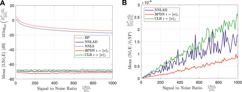
5.1.2 Noise-Blindness
Theorem 3.4 states that the NNLAD has an error bound similarly to the optimally tuned CLR and BPDN. Further, by Eq. 1 the ratio
should be bounded by some constant. To verify this, we fix the constants , , , , and vary the signal to noise ratio . For each we repeat Experiment 1 100 times. We plot the mean of the logarithmic relative -estimation error and the mean of the ratio of relative -estimation error and -noise power, i.e.
over the sparsity. The result can be found in Figures 3A,B .
The logarithmic relative -estimation errors of the different decoders stay in a constant relation to each other over the whole range of . This relation is roughly the relation we can find in Figure 1B for . As expected the the ratio of relative -estimation error and -noise power stays constant independent on the for all decoders. We deduce that the NNLAD is noise-blind. We repeat the experiment with and obtain Figures 4A,B.
Note that and not seems to be constant. Since is fairly small, we suspect that this is the result of CVX reaching a tolerance parameter2 and terminating, while the actual optimizer might in fact be the original signal. It is remarkable that even with the incredibly small signal to noise ratio of 10 the signal can be recovered by the NNLAD with an estimation error of for this noise distribution.
5.2 Decoding Complexity
5.2.1 Non-Negative Least Absolute Deviation Vs Iterative Methods
To investigate the convergence rates of the NNLAD as proposed in 4, we compare it to different types of decoders when . There are some sublinear time recovery methods for lossless expander matrices including ([3 Section 13.4, 5]). These are, as the name suggests, significantly faster than the NNLAD. These, as several other greedy methods ([3 Section 13.3, 5, 18, 19, 21]), rely on a strong lossless expansion property. As a representative of all greedy and sublinear time methods we will consider the EIHT, which has a linear convergence rate toward the signal and robust recovery guarantees ([3], Theorem 13.15). The EIHT also represents a best case benchmark. As a direct competitor we consider the NNLS implemented by the methods of [27] 3, which has a convergence rate of toward the optimal objective value. [27] can also be used to calculate the CLR if the residual norm is the -norm. However, calculating the projection onto the -ball in , is computationally slightly more complex than the projection onto . Thus, the CLR will be solved slightly slower than the NNLS with [27]. Note that cross-validation techniques would need to solve multiple optimization problems of a similar complexity as the NNLS to estimate a signal. As a consequence such methods have a multiple times higher complexity than the NNLS and are not considered here. As a worst case benchmark we consider a simple projected subgradient implementation of NNLAD using the Polyak step size, i.e.
which has a convergence rate of toward the optimal objective value ([33], Section 7.2.2 & Section 5.3.2). We initialized all iterated methods by 0. The EIHT will always use the parameter , the NNLAD and the NNLS the parameters and , see [27]. Just like the BPDN and CLR, the EIHT needs an oracle to get some unknown prior information, in this case . Parameters that can be computed from , will be calculated before the timers start. This includes the adjacency structure of for the EIHT, , for NNLAD, s, α for NNLS, since these are considered to be a part of the decoder. We will do the following experiment multiple times:
Experiment 2
1. If , generate a measurement matrix uniformly at random among all D-LRBG. If , draw each component of the measurement matrix independent and uniformly at random from , i.e., as Bernoulli random variables.
2. Generate a signal uniformly at random from .
3. Define the observation .
4. For each iterative method calculate the sequence of estimators for all and collect the relative estimation errors , the relative norms of the residuals and the time to calculate the first k iterations.
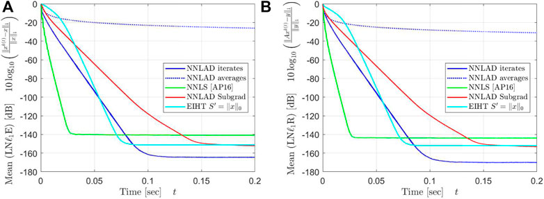
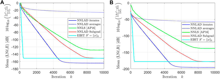
For this represents a biased sub-Gaussian random ensemble [13] with optimal recovery guarantees for the NNLS.For this represents a D-LRBG random ensemble with optimal recovery guarantees for the NNLAD. We fix the constants , , , , and repeat 2 100 times. We plot the mean of the logarithmic relative -estimation error and the mean of the relative -norm of the residual, i.e.
over the sparsity and the time. The result can be found in Figures 5, 6.
The averages of NNLAD converge significantly slower than the iterates, even though we lack a convergence rate for the iterates. We deduce that one should always use the iterates of NNLAD to recover a signal. Surprisingly, the averages converge even slower than the subgradient method. However, this is not because the averages converge slow, but rather because the subgradient method and all others converges faster than expected. In particular, the NNLAD iterates, EIHT and the NNLS all converge linearly toward the signal. Further, their correspoding objective values also converge linearly toward the optimal objective value. Even the subgradient method converges almost linearly. We deduce that the NNLS is the fastest of these methods if is a D-LRBG.
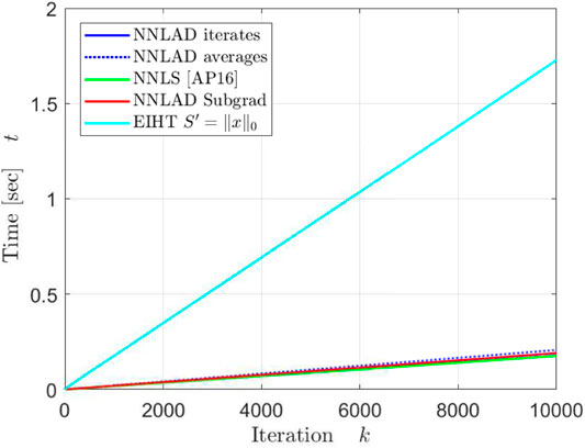
Apart from a constant the NNLAD iterates, EIHT and NNLS converge in the same order. However, this behavior does not hold if we consider a different distribution for as one can verify by setting each component as independent Bernoulli random variables. While EIHT has better iterations compared to the NNLS, it still takes more time to achieve the same estimation errors and residuals. We plot the mean of the time required to calculate the first k iterations in Figure 7.
The EIHT requires roughly 6 times as long as any other method to calculate each iteration. All methods but the EIHT can be implemented with only two matrix vector multiplications, namely once by and once by . Both of these requires roughly floating point operations. Hence, each iteration requires floating point operations. The EIHT only calculates one matrix vector multiplication, but also the median. This calculation is significantly slower than a matrix vector multiplication. For every we need to order a vector with D elements, which can be performed in . Hence, each iteration of EIHT requires floating point operations, which explains why the EIHT requires significantly more time for each iteration.
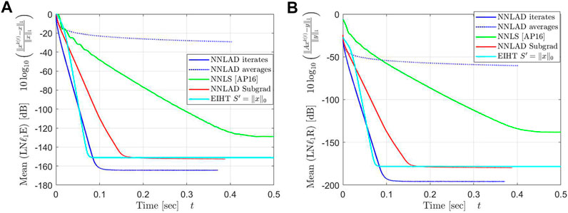
As we have seen the NNLS is able to recover signals faster than any other method, however it also only obeys sub-optimal robustness guarantees for uniformly at random chosen D-LRBG as we have seen in Figure 4A. We ask ourself whether or not the NNLS is also faster with a more natural measurement scheme, i.e., if are independent Bernoulli random variables. We repeat 2 100 times with for the NNLS and for the other methods. We again plot the mean of the logarithmic relative -estimation error and the mean of the relative -norm of the residual in Figures 8, 9.
The NNLAD and the EIHT converge to the solution with roughly the same time. Even the subgradient implementation of the NNLAD recovers a signal in less time than the NNLS. Further the convergence of NNLS does not seem to be linear anymore. We deduce that sparse structure of has a more significant influence on the decoding time than the smoothness of the data fidelity term. Also we deduce that even the subgradient method is a viable choice to recover a signal.
5.2.2 Non-Negative Least Absolute Deviation Vs SPGL1
As a last test we compare the NNLAD to the SPGL1 [16, 34] toolbox for matlab.
Experiment 3
1. Draw the measurement matrix uniformly at random among all D-LRBG.
2. Generate the signal uniformly at random from .
3. Define the observation .
4. Use a benchmark decoder to calculate an estimator and collect the relative estimation errors and the time to calculate .
5. For each iterative method calculate iterations until and . Collect the time to perform these iterations. If this threshold can not be reached after iterations, the recovery failed and the time is set to .
We again fix the dimension , , and vary . For both the BP implementation of SPGL1 and the CLR implementation of SPGL1 we repeat Experiment 3 100 times for each S. We plot the mean of the time to calculate the estimators and plot these over the sparsity in Figures 10A,B.
The NNLAD implementation is slower than both SPGL1 methods for small S. However, if we have the optimal number of measurements , the NNLAD is faster than both SPGL1 methods.
5.2.3 Summary
The implementation of NNLAD as presented in Algorithm 1 is a reliable recovery method for sparse non-negative signals. There are methods that might be faster, but these either recover a smaller number of coefficients (EIHT, greedy methods) or they obey sub-optimal recovery guarantees (NNLS). The implementation is as fast as the commonly uses SPGL1 toolbox, but has the advantage that it requires no tuning depending on the unknown or . Lastly, the NNLAD can handle peaky noise overwhelmingly good.
5.3 Application for Viral Detection
With the outbreak and rapid spread of the COVID-19 virus we need to test a large amount of people for an infection. Since we can only test a fixed number of persons in a given time, the number of persons tested for the virus grows at most linearly. On the other hand, models suggest that the number of possibly infected persons grows exponentially. At some point, if that is not already the case, we will have a shortage of test kits and we will not be able to test every person. It is thus desirable to test as much persons with as few as possible test kits.
The field group testing develops strategies to test groups of individuals instead of individuals in order to reduce the amount of tests required to identify infected individuals. The first advances in group testing were made in [35]. For a general overview about group testing we refer to [36].
The problem of testing a large group for a virus can be modeled as a compressed sensing problem in the following way: Suppose we want to test N persons, labeled by , to check whether or not they are affected by a virus. We denote by the quantity of viruses in the specimen of the nth person. Suppose we have M test kits, labeled by . By we denote the amount of viruses in the sample of the mth test kit. Let . For every n we put a fraction of size of the specimen of the nth person into the sample for the mth test kit. The sample of the mth test kit will then have the quantity of viruses
where is the amount of viruses in the sample originating from a possible contamination of the sample. A quantitative reverse transcription polymerase chain reaction estimates the quantity of viruses by with a small error . After all M tests we detect the quantity
where . Since contamination of samples happens rarely, is assumed to be peaky in terms of Table 1, while is assumed to have even mass but a small norm. In total is peaky.
Often each specimen is tested separately, meaning that is the identity. In particular, we need at least as much test kits as specimens. Further, we estimate the true quantity of viruses by , which results in the estimation error . Since the noise vector is peaky, some but few tests will be inaccurate and might result in false positives or false negatives.
In general, only a fraction of persons is indeed affected by the virus. Thus, we assume that for some small S. Since the amount of viruses is a non-negative value, we also have . Hence, we can use the NNLR to estimate and in particular we should use the NNLAD due to the noise being peaky. Corollary 3.6 suggests to choose as the random walk matrix of a lossless expander or by ([3], Theorem 13.7) to choose as a uniformly at random chosen D-LRBG. Such a matrix has non-negative entries and the column sums of are not greater than one. This is a necessary requirement since each column sum is the total amount of specimen used in the test procedure. Especially, a fraction of of each specimen is used in exactly D test kits.
By Corollary 3.6 and [ [3], Theorem 13.7] this allows us to reduce the number of test kits required to . As we have seen in Figures 4A,B we expect the NNLAD estimator to correct the errors from and the estimation error to be in the order of which is assumed to be small. Hence, the NNLAD estimator with a random walk matrix of a lossless expander might even result in less false positives and false negatives than individual testing.
Note that the lack of knowledge about the noise favors the NNLAD recovery method over a (BPDN) approach. Further, since the total sum of viruses in all patients given by is unknown, it is undesirable to use (CLR).
Data Availability Statement
The original contributions presented in the study are included in the article/Supplementary Material, further inquiries can be directed to the corresponding author.
Author Contributions
BB and PJ proposed the research problem. HP derived the results of the paper, with feedback from BB and PJ. HP wrote the paper also with feedback from BB and PJ.
Funding
The work was partially supported by DAAD grant 57417688. PJ has been supported by DFG grant JU 2795/3. BB has been supported by BMBF through the German Research Chair at AIMS, administered by the Humboldt Foundation. We acknowledge support by the German Research Foundation and the Open Access Publication Funds of TU Berlin. This article has appeared as a preprint (27), see https://arxiv.org/abs/2003.13092.
Conflict of Interest
The authors declare that the research was conducted in the absence of any commercial or financial relationships that could be construed as a potential conflict of interest.
Footnotes
1The -constrained least residual is given by for some norm .
2The tolerance parameters of CVX are the second and fourth root of the machine precision by default [30, 31].
3This was the fastest method found by the authors. Other possibilities would be [15, Algorithm 2], [26].
References
1. Candes, EJ, Romberg, J, and Tao, T. Robust Uncertainty Principles: Exact Signal Reconstruction from Highly Incomplete Frequency Information. IEEE Trans Inf Theory (2006). 52:489–509. doi:10.1109/TIT.2005.862083
CrossRef Full Text | Google Scholar
3. Foucart, S, and Rauhut, H. A Mathematical Introduction to Compressive Sensing. Basel, Switzerland: Birkhäuser (2013).
4. Hastie, T, Tibshirani, R, and Wainwright, M. Statistical Learning with Sparsity: The Lasso and Generalizations. New York, NY: Chapman and Hall/CRC (2015).
5. Donoho, DL, and Tanner, J. Sparse Nonnegative Solution of Underdetermined Linear Equations by Linear Programming. Proc Natl Acad Sci (2005). 102:9446–51. doi:10.1073/pnas.0502269102
PubMed Abstract | CrossRef Full Text | Google Scholar
6. Gilbert, A, and Indyk, P. Sparse Recovery Using Sparse Matrices. Proc IEEE (2010). 98:937–47. doi:10.1109/JPROC.2010.2045092
CrossRef Full Text | Google Scholar
7. Bruckstein, AM, Elad, M, and Zibulevsky, M. On the Uniqueness of Non-negative Sparse & Redundant Representations. Proc IEEE Int Conf Acoust Speech Signal Process (2008). 5145–8. doi:10.1109/ICASSP.2008.4518817
CrossRef Full Text | Google Scholar
8. Donoho, DL, and Tanner, J. Counting the Faces of Randomly-Projected Hypercubes and Orthants, with Applications. Discrete Comput Geom (2010). 43:522–41. doi:10.1007/s00454-009-9221-z
CrossRef Full Text | Google Scholar
9. Wang, M, Xu, W, and Tang, A. A Unique “Nonnegative” Solution to an Underdetermined System: From Vectors to Matrices. IEEE Trans Signal Process (2011). 59:1007–1016. doi:10.1109/TSP.2010.2089624
CrossRef Full Text | Google Scholar
10. Slawski, M, and Hein, M. Sparse Recovery by Thresholded Non-negative Least Squares. Adv Neural Inf Process Syst (2011). 24:1926–1934.
Google Scholar
11. Slawski, M, and Hein, M. Non-negative Least Squares for High-Dimensional Linear Models: Consistency and Sparse Recovery without Regularization. Electron J Stat (2013). 7:3004–3056. doi:10.1214/13-EJS868
CrossRef Full Text | Google Scholar
12. Kabanava, M, Kueng, R, Rauhut, H, and Terstiege, U. Stable Low-Rank Matrix Recovery via Null Space Properties. Inf Inference (2016). 5:405–441. doi:10.1093/imaiai/iaw014
CrossRef Full Text | Google Scholar
13. Kueng, R, and Jung, P. Robust Nonnegative Sparse Recovery and the Nullspace Property of 0/1 Measurements. IEEE Trans Inf Theory (2018). 64:689–703. doi:10.1109/TIT.2017.2746620
CrossRef Full Text | Google Scholar
14. Shadmi, Y, Jung, P, and Caire, G. Sparse Non-negative Recovery from Biased Subgaussian Measurements Using NNLS. In: IEEE International Symposium on Information Theory; 2019 July 7–12; Paris, France (2019).
CrossRef Full Text | Google Scholar
15. Chambolle, A, and Pock, T. A First-Order Primal-Dual Algorithm for Convex Problems with Applications to Imaging. J Math Imaging Vis (2011). 40:120–45. doi:10.1007/s10851-010-0251-1
CrossRef Full Text | Google Scholar
16. Van Den Berg, E, and Friedlander, MP. Probing the Pareto Frontier for Basis Pursuit Solutions. SIAM J Sci Comput (2009). 31:890–912. doi:10.1137/080714488
CrossRef Full Text | Google Scholar
17. Bühlmann, P, and Van De Geer, S. Statistics for High-Dimensional Data. Berlin, Heidelberg: Springer (2011).
18. Jafarpour, S, Xu, W, Hassibi, B, and Calderbank, R. Efficient and Robust Compressed Sensing Using Optimized Expander Graphs. IEEE Trans Inf Theory (2009). 55:4299–4308. doi:10.1109/TIT.2009.2025528
CrossRef Full Text | Google Scholar
19. Xu, W, and Hassibi, B. Efficient Compressive Sensing with Deterministic Guarantees Using Expander Graphs. In: IEEE Information Theory Workshop; 2007 September 2–6; Tahoe City, CA, United States (2007). 414–9.
Google Scholar
20. Berinde, R, Gilbert, AC, Indyk, P, Karloff, H, and Strauss, MJ. Combining Geometry and Combinatorics: A Unified Approach to Sparse Signal Recovery. In: 46th Annual Allerton Conference on Communication; 2008 September 23–26; Monticello, IL, United States (2008). 798–805.
Google Scholar
21. Khajehnejad, MA, Dimakis, AG, Xu, W, and Hassibi, B. Sparse Recovery of Nonnegative Signals with Minimal Expansion. IEEE Trans Signal Process (2011). 59:196–208. doi:10.1109/TSP.2010.2082536
CrossRef Full Text | Google Scholar
22. Morgenshtern, VI, and Candès, EJ. Super-resolution of Positive Sources: The Discrete Setup. SIAM J Imaging Sci (2016). 9:412–44. doi:10.1137/15M1016552
CrossRef Full Text | Google Scholar
23. Jaensch, F, and Jung, P. Robust Recovery of Sparse Nonnegative Weights from Mixtures of Positive-Semidefinite Matrices(Preprint). (2020). Available from: https://arxiv.org/abs/2003.12005.
25. Nesterov, Y Introductory Lectures on Convex Optimization - A Basic CourseApplied Optimization. New York, NY: Springer (2004).
CrossRef Full Text
26. Beck, A, and Teboulle, M. A Fast Iterative Shrinkage-Thresholding Algorithm for Linear Inverse Problems. SIAM J Imaging Sci (2009). 2:183–202. doi:10.1137/080716542
CrossRef Full Text | Google Scholar
27. Attouch, H, and Peypouquet, J. The Rate of Convergence of Nesterov's Accelerated Forward-Backward Method Is Actually Faster Than $1/k^2$. SIAM J Optim (2016). 26:1824–1834. doi:10.1137/15M1046095
CrossRef Full Text | Google Scholar
29. Kümmerle, C. Understanding and Enhancing Data Recovery Algorithms- From Noise-Blind Sparse Recovery to Reweighted Methods for Low-Rank Matrix Optimization. [PhD dissertation]. München (Germany): Technical University of Munich (2019).
30. Grant, M, and Boyd, S. CVX: Matlab Software for Disciplined Convex Programming (2014).
31. Grant, MC, and BOYd, SP. Graph Implementations for Nonsmooth Convex Programs. In: V Blondel, S Boyd, and H Kimura, editors. Recent Advances in Learning and Control. Lecture Notes in Control and Information Sciences. New York, NY: Springer-Verlag Limited (2008). p. 95–110.
Google Scholar
32. Dirksen, S, Lecué, G, and Rauhut, H. On the Gap between Restricted Isometry Properties and Sparse Recovery Conditions. IEEE Trans Inf TheorY (2018). 64:5478–87. doi:10.1109/TIT.2016.2570244
CrossRef Full Text | Google Scholar
33. Polyak, BT. Introduction to Optimization (Translations Series in Mathematics and Engineering). New York, NY: Optimization Software, Inc (1987).
34. Van Den Berg, E, and Friedlander, MP. SPGL1: A Solver for Large-Scale Sparse Reconstruction (2019).
35. Dorfman, R. The Detection of Defective Members of Large Populations. Ann Math Statist 14 (1943). 436–40. doi:10.1214/aoms/1177731363
CrossRef Full Text | Google Scholar
36. Aldridge, M, Johnson, O, and Scarlett, J. Group Testing: An Information Theory Perspective. FNT Commun Inf Theory (2019). 15:196–392. doi:10.1561/0100000099
CrossRef Full Text | Google Scholar
37. Petersen, HB, and Jung, P. Robust Instance-Optimal Recovery of Sparse Signals at Unknown Noise Levels(Preprint) (2020). Available from: https://arxiv.org/abs/2008.08385.
6 Appendix
6.1 Proof of Non-Negative Least Residual Recovery Guarantee
By we denote the all ones vector in or respectively. The proof is an adaption of the steps used in [13]. As for most convex optimization problems in compressed sensing we use ([3], Theorem 4.25) and [ [3], Theorem 4.20] respectively, which require to have the RNSP.
Theorem 6.1 ([3], Theorem 4.25) and ([3], Theorem 4.20)). Let and suppose has the -RNSP of order S with respect to with constants ρ and τ. Then, it holds that
If , this bound can be improved to
Note that by a modification of the proof this result also holds for . The modifications on the proofs of ([3], Theorem 4.25) and ([3], Theorem 4.20) are straight forward, only the modification of ([3], Theorem 2.5) might not be obvious. See also [37]. As a consequence, all our statements also hold for with . If is a diagonal matrix, we can calculate some operator norms fairly easy:
We use this relation at several places throughout this section. Furthermore, we use ([13], Lemma 5) without adaption. For the sake of completeness we add a short proof.
Lemma 6.2 ([13], Lemma 5). Let and suppose that has -RNSP of order S with respect to with constants ρ and τ. Let be a diagonal matrix with . If , then has -RNSP of order S with respect to with constants and .
Proof Let and . If we apply the RNSP of for the vector , we get
This finishes the proof.
Next we adapt ([13], Theorem 4) to account for arbitrary norms. Further, we obtain a slight improvement in form of the dimensional scaling constant . With this, our error bound becomes for asymptotically the error bound of the basis pursuit denoising, whenever and [3].
Proposition 6.3 (Similar to ([13], Theorem 4)). Let and be a norm on with dual norm . Suppose has -RNSP of order S with respect to with constants ρ and τ. Suppose has the criterion with vector and constant κ and that . Then, we have
If , this bound can be improved to
Proof Let . In order to apply Lemma 6.2 we set as the matrix with diagonal and zero else. It follows that and . We can apply Lemma 6.2, which yields that has -RNSP with constants and . We apply Theorem 6.1 with the matrix , the vectors , and the constants and and get
We lower bound the left hand side further to get
We want to estimate the term using the criterion. Since , and is a diagonal matrix, we have
Applying this to Eq. 5 we get
If we can repeat the proof with the improved bound of Theorem 6.1.
After these auxiliary statements it remains to prove the main result of Section 3 about the properties of the NNLR minimizer.
Proof of Theorem 3.4. By applying Proposition 6.3 with and we get
 Hendrik Bernd Petersen
 Bubacarr Bah
 Peter Jung