A New Nonparametric Estimate of the Risk-Neutral Density with Applications to Variance Swaps

Estimates of risk-neutral densities of future asset returns have been commonly used for pricing new financial derivatives, detecting profitable opportunities, and measuring central bank policy impacts. We develop a new nonparametric approach for estimating the risk-neutral density of asset prices and reformulate its estimation into a double-constrained optimization problem. We evaluate our approach using the S&P 500 market option prices from 1996 to 2015. A comprehensive cross-validation study shows that our approach outperforms the existing nonparametric quartic B-spline and cubic spline methods, as well as the parametric method based on the normal inverse Gaussian distribution. As an application, we use the proposed density estimator to price long-term variance swaps, and the model-implied prices match reasonably well with those of the variance future downloaded from the Chicago Board Options Exchange website.

1 Introduction

A financial derivative, such as option, swap, future, or forward contract, is an asset that is contingent on an underlying asset. Its fair price can be obtained by calculating the expected future payoff under a risk-neutral probability distribution. Therefore, the problem of pricing a derivative can be addressed via estimating the risk-neutral density (RND) of the future payoff of the underlying asset. The estimated prices, known as fair prices, may help companies and investors to avoid financial risk or detect profitable opportunities, especially on over-the-counter (OTC) securities. The estimated risk-neutral distribution can be further used by, for example, central banks to infer market belief on economic events of interest and measure impacts of monetary policies [1–3]. On the other hand, the market prices of the derivatives traded in a financial market reveal information about the RND. Breeden and Litzenberger (1978) [4] were among the first to use option prices to estimate the risk-neural probability distribution of the future payoff of the underlying asset. Among the financial products that can be used to recover the RND, European options are the most common ones, which give the investors rights to trade assets at a preagreed price (i.e., strike price) at the maturity date. Among all the underlying assets that options are written on, Standard and Poor’s 500 Index (S&P 500) is a popular one, which aggregates the values of stocks of 500 large companies traded on American stock exchanges and provides a credible view of the American stock market for investors.

There are a plethora of approaches toward recovering RND functions in the literature (see, for example, [5], for an extensive review). Parametric approaches typically specify a statistical model for the RND and the structural parameters are recovered by solving an optimization problem. For instance, a lognormal distribution was used in [6]; a mixture of lognormal distributions proposed by [7] was considered in [2]; and a three-parameter Burr distribution was employed in [8], called the Burr family, which covers a broad range of shapes, including distributions similar to gamma, lognormal, and J-shaped beta. Another commonly used probability distribution in the literature of derivative pricing is the generalized hyperbolic distribution that contains variance gamma, normal inverse Gaussian (NIG), and t distributions as special cases (see, for instance, [9, 10]).

Nonparametric procedures, by contrast, are free from distributional assumptions on the underlying asset and thus achieve more flexibility than parametric methods. For example, in [11], cubic spline functions to model the unknown RND were used. An estimated density is numerically obtained by solving a quadratic programming problem with a convex objective function and nonnegativity constraints. The authors deliberately chose more knots than option strikes for higher flexibility. Lee (2014) [12] approximated the risk-neutral cumulative distribution function using quartic B-splines with power tails and the minimum number of knots that meet zero bid-ask spread. Their estimation was based on out-of-the-money option prices.

In this article, we propose a simpler but more powerful nonparametric solution using piecewise constant (PC) functions to estimate the RND. It is easy to implement since the estimating problem is formulated as a weighted least squared (WLS) procedure. It is more powerful since our method can recover the RND more effectively with all available option market prices without screening. Furthermore, our solution provides a practical way to explore profitable investment opportunities in financial markets by comparing the estimated prices and corresponding market prices.

The rest of this article is structured as follows. In Materials and Methods, we introduce the proposed nonparametric approach after reviewing cubic splines, quartic B-splines, and the NIG parametric approaches in the literature. In Pricing European Options, we run comprehensive cross-validation studies using the S&P 500 European option data to compare different methods and provide theoretical justifications on the consistency of our estimator for fair option prices. In Pricing Variance Swap, we apply the proposed nonparametric approach to price variance swaps, which is challenging in practice [13, 14]. We conclude in Discussion. The proofs and more formulae are collected in the Supplementary Material.

2 Materials and Methods

In this section, we first provide a brief review of the cubic splines, quartic B-splines, and NIG approaches in the literature for recovering the RND. Then, we introduce the proposed PC nonparametric approach with least square (LS) and WLS procedures.

2.1 Nonnegative Cubic Spline Estimate for RND

Given the current trading date t and the expiration date T of European options, let $[K_1,K_q]$ be the range of strike prices of all available options traded in the market with the same underlying asset. Monteiro et al. (2008) [11] considered $s+1$ equally spaced knots for a cubic spline with $K_1=x_1<x_2<x_3<\cdots <x_s<x_{s+1}=K_q$. These knots are not necessarily a subset of the available strikes. Nevertheless, the closer these knots are to the strikes, the better their solution is. They also claimed that the number of knots should not be very much larger than the number of distinct strikes.

For the sake of nonnegativity of the estimated RNDs, in [11], the solution is much more complicated and computationally expensive than the usual cubic spline estimates. For comparison purposes, we keep only the constraints that ensure the nonnegativity of the density function on knots in their optimization procedure. By evaluating the difference between the estimated fair prices and the market prices of options, if our approach achieves higher accuracy than the cubic spline estimate with fewer constraints, then our approach is considered to be superior to that of [11].

When it comes to practical implementation [11], eliminating option prices is suggested that led to potential arbitrage opportunities according to the bid-ask interval, put-call parity, monotonicity, and strict convexity. They also generated “fake” call option prices using put-call parity to eliminate “artificial” arbitrage opportunities. Our comprehensive studies in Pricing European Options show that their screening and cleaning procedure may result in substantial information loss.

2.2 Quartic B-Spline Estimate

Lee (2014) [12] adopted a uniform quartic B-spline to estimate the risk-neutral cumulative distribution function (CDF). They used power tails to extrapolate outside the strike price range. They suggested using only the out-of-the-money (hereafter, OTM) options to estimate the CDF, including OTM call options whose strikes are higher than the underlying asset price and OTM put options whose strikes are lower than the underlying asset price. OTM options are typically cheaper than in-the-money (ITM) options and are considered to be more liquid as well. Nevertheless, our case studies in Pricing European Options show that ITM options may help recover the RND as well.

Due to fewer parameters, the quartic B-spline estimate is computationally more efficient than the nonnegative cubic spline approach. Lee (2014) [12] chose the number of knots needed as the minimum number that satisfies zero bid-ask pricing spread. They also suggested eliminating options that violate monotonicity and strict convexity constraints.

2.3 NIG Parametric Approach

For comparison purposes, we choose one parametric approach for approximating the RND, as suggested by [9, 15]. It is based on the NIG distribution, which belongs to the generalized hyperbolic class and can be characterized by its first four moments, i.e., mean, variance, skewness, and kurtosis. According to [16], these four moments can be estimated by the OTM European call and put options. One major issue with NIG density estimate is that, as shown in [10], the feasibility of NIG approach drops down as the time-to-maturity increases since more estimated skewness and kurtosis pairs fall outside the feasible domain of the NIG distribution.

2.4 The Proposed Piecewise Constant Nonparametric Approach

The PC approach that we propose in this article is nonparametric by nature. It is simpler but more efficient. Let $S_t$ and $S_T$ stand for the current price of equity on day t and the future price on day T. To estimate the RND function $f_{\mathbb{Q}}$ of $\text{log}\left(S_T\right)$ conditional on the information up to day t, we propose to use a PC function, or a step function, to approximate $f_{\mathbb{Q}}$, with all distinct strike prices as knots. The constants in the step function are estimated by solving an optimization problem subject to certain constraints. By forcing the constants to be nonnegative, the nonnegativity of the estimated RND is guaranteed.

To be precise, suppose that we have a collection of market prices of European put and call options that are traded on date t and expire on date T. Let $\left\{K_1,K_2,\dots ,K_q\right\}$ represent the distinct strikes in ascending order and $\mathcal{C}$ be the collection of indices for call options and $\mathcal{P}$ for put options. Then, $\mathcal{C}{{\displaystyle \cup }}^{\text{}}\mathcal{P}=\left\{\mathrm{1,2},\dots ,q\right\}$. Let $m=\left|\mathcal{C}\right|$ and $n=\left|\mathcal{P}\right|$ be the numbers of calls and puts, respectively. Then $m+n\ge q$.

Given a RND $f_{\mathbb{Q}}$, the fair prices of put option and call option with strike $K_i$ are

$\begin{array}{l}{P}_i={\mathbb{E}}_t^{\mathbb{Q}}{e}^{-R_{tT}}{\left(K_i-S_T\right)}_{+}=e^{-R_{tT}}{{\displaystyle \int }}_{-\infty }^{\log K_i}\left(K_i-e^y\right)f_{\mathbb{Q}}\left(y\right)dy,\\ C_i={\mathbb{E}}_t^{\mathbb{Q}}{e}^{-R_{tT}}{\left(S_T-K_i\right)}_{+}=e^{-R_{tT}}{{\displaystyle \int }}_{\log K_i}^{\infty }\left(e^y-K_i\right)f_{\mathbb{Q}}\left(y\right)dy,\end{array}$

respectively, where $R_{tT}$ stands for the cumulative risk-free interest rate from t to T; that is, $1 on day t ends for sure with $e^{R_{tT}}$ dollars on day T. We denote by $r_t$ the risk-free interest rate over the period $[t,t+1]$, which is obtained from the risk-free zero-coupon bond, and clearly $R_{tT}={{\displaystyle \sum }}_{j=t}^{T-1}{r}_j$.

To account for the RND outside the range $[K_1,K_q]$, we add $K_0=K_1/c_K$ and $K_{q+1}=c_K{K}_q$, where $c_K>1$ is a predetermined constant that can be chosen by means of cross-validation or prior knowledge (see details in Pricing European Options). We then use a PC function $f_{\text{Δ}}$ to approximate $f_{\mathbb{Q}}$; that is,

$f_{\text{Δ}}\left(y\right)=a_l,\text{ for\hspace{1em}}\log K_{l-1}<y\le \log K_l,l=\mathrm{1,2},\dots ,q+1,(1)$

and zero elsewhere. Here, $\text{Δ}=\left\{\text{log}{K}_1,\dots ,\text{log}{K}_q\right\}$ stands for the collection of distinct strikes in log scale and $\left\{a_l,l=1,\dots ,q+1\right\}$ are nonnegative constants satisfying

${\displaystyle \sum }_{l=1}^{q+1}{a}_l\log \frac{K_l}{K_{l-1}}=1(2)$

due to the condition ${{\displaystyle \int }}_{-\infty }^{+\infty }{f}_{\text{Δ}}\left(y\right)dy=1$.

Given the approximate RND $f_{\text{Δ}}$, the estimated put and call prices with strike $K_i$ are

${\widehat{P}}_i=e^{-R_{tT}}{{\displaystyle \int }}_{-\infty }^{\text{log}{K}_i}\left(K_i-e^y\right)f_{\text{Δ}}\left(y\right)dy,(3)$

${\widehat{C}}_i=e^{-R_{tT}}{{\displaystyle \int }}_{\text{log}{K}_i}^{\infty }\left(e^y-K_i\right)f_{\text{Δ}}\left(y\right)dy,(4)$

respectively, which are essentially linear functions of $a_1,\dots ,a_q$.

Proposition 2.1. Given $a_l\ge 0,l=1,\dots ,q+1$ satisfying Eq. 2, the estimated prices for put and call options with strike $K_i$ satisfy

$e^{R_{tT}}{\widehat{P}}_i=a_1{X}_{i,1}^{\left(P\right)}+\cdots +a_q{X}_{i,q}^{\left(P\right)}+X_{i,q+1}^{\left(P\right)},(5)$

$e^{R_{tT}}{\widehat{C}}_i=a_1{X}_{i,1}^{\left(C\right)}+\cdots +a_q{X}_{i,q}^{\left(C\right)}+X_{i,q+1}^{\left(C\right)},(6)$

where$X_{i,l}^{\left(P\right)}=X_{i,l}^{\left(p\right)}-\log \left(K_l/K_{l-1}\right){\left(\log c_K\right)}^{-1}{X}_{i,q+1}^{\left(p\right)}$,$X_{i,l}^{\left(C\right)}=X_{i,l}^{\left(c\right)}-\text{log}\left(K_l/K_{l-1}\right)$${\left(\log c_K\right)}^{-1}$$X_{i,q+1}^{\left(c\right)}$,$l=\mathrm{1,2},\dots ,q$;$X_{i,q+1}^{\left(P\right)}=X_{i,q+1}^{\left(p\right)}{\left(\log c_K\right)}^{-1}$,$X_{i,q+1}^{\left(C\right)}=X_{i,q+1}^{\left(c\right)}$${\left(\log c_K\right)}^{-1}$; and$X_{i,l}^{\left(p\right)}=\left[K_i\log \left(K_l/K_{l-1}\right)-\left(K_l/K_{l-1}\right)\right]\cdot 1\left(K_i\ge K_l\right)$,$X_{i,l}^{\left(c\right)}=\left[\left(K_l-K_{l-1}\right)-K_i\log \left(K_l-K_{l-1}\right)\right]\cdot 1\left(K_i<K_l\right)$,$l=\mathrm{1,2},\dots ,q+1$.

The proof of Proposition 2.1 is relegated to Supplementary Material A.

The unknown parameters $a_1,\dots ,a_{q+1}$ are estimated by minimizing the following LS objective function:

$L\left(a_1,\dots ,a_{q+1}\right)=\frac{1}{m+n}\left[{\displaystyle \sum }_{i\in \mathcal{C}}{\left({\widehat{C}}_i-{\tilde{C}}_i\right)}^2+{\displaystyle \sum }_{i\in \mathcal{P}}{\left({\widehat{P}}_i-{\tilde{P}}_i\right)}^2\right](7)$

subject to $a_l\ge 0$, $l=\mathrm{1,2},\dots ,q+1$, and Eq. 2, where ${\tilde{C}}_i$ and ${\tilde{P}}_i$ are market prices of call option and put option, respectively, with strike $K_i$ . If there exists an RND $f_{\mathbb{Q}}$, we have $C_i={\tilde{C}}_i,i\in \mathcal{C}$ and $P_i={\tilde{P}}_i,i\in \mathcal{P}$. That is, market prices are fair if there is no arbitrage in the financial market.

From an investment point of view, because a more expensive option tends to be less liquid, an alternative approach to determining $a_1,\dots ,a_{q+1}$ is to minimize a WLS objective function:

$W\left(a_1,\dots ,a_{q+1}\right)=\frac{1}{m+n}\left[{\displaystyle \sum }_{i\in \mathcal{C}}{\left(\frac{{\widehat{C}}_i-{\tilde{C}}_i}{{\tilde{C}}_i}\right)}^2+{\displaystyle \sum }_{i\in \mathcal{P}}{\left(\frac{{\widehat{P}}_i-{\tilde{P}}_i}{{\tilde{P}}_i}\right)}^2\right].(8)$

The WLS estimate is in favor of OTM options over ITM options in that OTM options are typically less expensive and more liquid.

3 Pricing European Options

In this section, we use the S&P 500 European options to evaluate the performances of various RND estimators.

3.1 S&P 500 European Option Data

We consider European calls and puts written on the S&P 500 indices from January 2, 1996, to August 31, 2015, in the United States [10, 14]. The expiration dates are the third Saturday of the delivery month. Following [14], we keep only the options with positive bid prices and positive volumes and with expiration date of more than seven days in our analysis. Similar to [10], we categorize options into seven groups with expiration in $7\sim 14$, $17\sim 31$, $81\sim 94$, $171\sim 199$, $337\sim 393$, $502\sim 592$, and $670\sim 790$ days, respectively, for the purpose of examining the effects of the length of maturity on pricing. The numbers of options and $\left(t,T\right)$ pairs under consideration are presented in Table 1.

TABLE 1

TABLE 1. Numbers of calls, puts, and $\left(t,T\right)$ pairs in different time-to-maturity categories (number of days to expiration).

3.2 Comprehensive Comparisons With Existing Methods

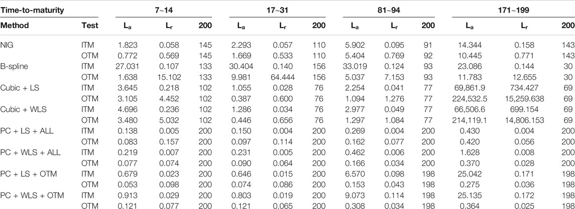
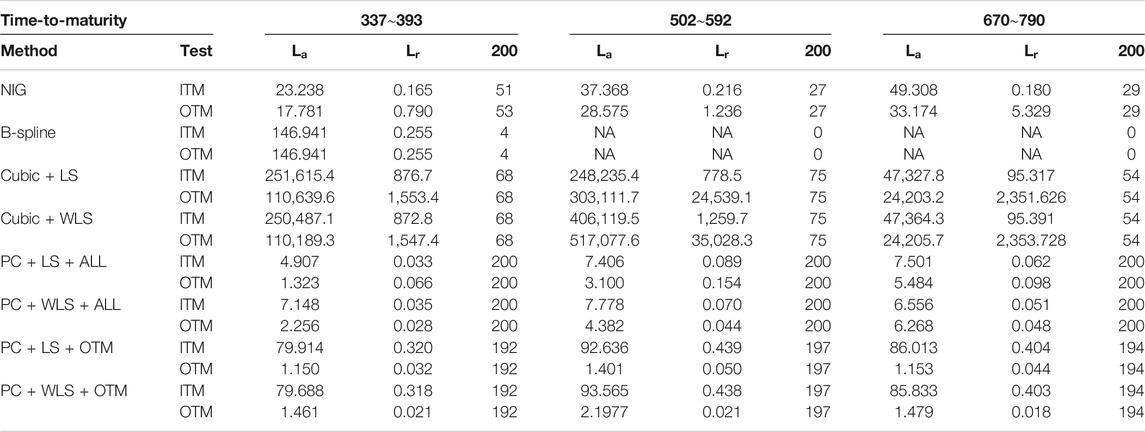
We use the S&P 500 European options to evaluate the performance of the following methods: the parametric NIG estimate, the quartic B-spline (B-spline) estimate, the nonnegative cubic spline estimates with either LS criterion (cubic + LS) or WLS criterion (cubic + WLS), and the proposed PC estimate with either LS or WLS objective function using OTM options only (PC + LS + OTM or PC + WLS + OTM) or using all available options (PC + LS + ALL or PC + WLS + ALL). All the comparisons are made based on their ability to recover option market prices.

For each of the seven time-to-maturity categories listed in Table 1, we randomly selected 200 pairs of $\left(t,T\right)$. For each pair, the market prices of calls and puts are collected. The aforementioned approaches are applied to estimate the RND of the underlying asset at time T. We then use the estimated RND to obtain ${\widehat{C}}_i$ and ${\widehat{P}}_i$ . The discrepancy between the market prices and the estimated prices is assessed by means of the absolute error $L_a$ and the relative error $L_r$ defined as follows:

$\begin{array}{l}{L}_a^2=\frac{1}{\left|{\mathcal{C}}_t\right|+\left|{\mathcal{P}}_t\right|}\left[{\displaystyle \sum }_{i\in {\mathcal{C}}_t}{\left({\widehat{C}}_i-{\tilde{C}}_i\right)}^2+{\displaystyle \sum }_{i\in {\mathcal{P}}_t}{\left({\widehat{P}}_i-{\tilde{P}}_i\right)}^2\right],\\ L_r^2=\frac{1}{\left|{\mathcal{C}}_t\right|+\left|{\mathcal{P}}_t\right|}\left[{\displaystyle \sum }_{i\in {\mathcal{C}}_t}{\left({\widehat{C}}_i/{\tilde{C}}_i-1\right)}^2+{\displaystyle \sum }_{i\in {\mathcal{P}}_t}{\left({\widehat{P}}_i/{\tilde{P}}_i-1\right)}^2\right],\end{array}$

where ${\mathcal{C}}_t$ (or ${\mathcal{P}}_t$) refers to the collection of indices of call (or put) options used for testing purposes. In Table 2 and Table 3, we choose ${\mathcal{C}}_t$ and ${\mathcal{P}}_t$ to be either all available OTM options or ITM options. We report the average $L_a$ and $L_r$ over the 200 randomly selected pairs of $\left(t,T\right)$ for each estimation approach. The columns labeled ‘200’ show the actual number of pairs that yield a valid RND estimate. The higher the count, the more effective the method. As explained in Section 2.3, the NIG approach is quite picky in selecting calls and puts. For B-spline and cubic methods, following the same filtering procedures as in [11, 12], respectively, we observe that fewer options become available as the time-to-maturity increases, which results in substantial information loss. On the contrary, our PC methods with LS or WLS are feasible for almost all cases, especially when using both ITM and OTM options.

TABLE 2

TABLE 2. Comprehensive comparison of different RND estimates: part I.

TABLE 3

TABLE 3. Comprehensive comparison of different RND estimates: part II.

In terms of the absolute error $L_a$ and the relative error $L_r$ computed for different combinations of time-to-maturities and RND estimates, our PC estimates are more stable and accurate than the other three approaches. As illustrated in Tables 2, 3, the proposed PC methods always yield the lowest $L_a$ or $L_r$, regardless of the type of options used. In order for a cross-sectional comparison to be conducted among all the approaches, only OTM options are considered when using the proposed PC approach to price options (i.e., PC + LS + OTM or PC + WLS + OTM). In practice, however, we would recommend using all available option prices, including both ITM and OTM options. In particular, if the goal is to obtain the most precise price, we recommend ‘PC + LS + ALL’ in that it controls absolute error $L_a$ the best; if one seeks a higher return on investment, we would recommend ‘PC + WLS + ALL’ instead, which controls relative error $L_r$ the best.

3.3 Consistency of PC Estimates for Fair Prices

Given distinct strike prices $K_1<K_2<\cdots <K_q$, the associated market prices of calls and puts, $\left\{{\tilde{C}}_i,i\in \mathcal{C}\right\}$ and $\left\{{\tilde{P}}_i,i\in \mathcal{P}\right\}$, respectively, traded on date t with expiration date T satisfy

${\tilde{C}}_i=e^{-R_{tT}}{{\displaystyle \int }}_{\text{log}{K}_i}^{\infty }\left(e^y-K_i\right)f_{\mathbb{Q}}\left(y\right)dy,{\tilde{P}}_i=e^{-R_{tT}}{{\displaystyle \int }}_{-\infty }^{\text{log}{K}_i}\left(K_i-e^y\right)f_{\mathbb{Q}}\left(y\right)dy,(9)$

provided that RND $f_{\mathbb{Q}}$ of $\text{log}{S}_T$ exists. That is, the market prices $\left({\tilde{C}}_i,{\tilde{P}}_i\right)$ agree with the fair prices $\left(C_i,P_i\right)$ .

According to Eq. 1, the proposed PC approach provides the following approximation:

$f_{\text{Δ}}\left(x\right)={\displaystyle \sum }_{l=1}^{q+1}{a}_l{1}_{\left(\log K_{l-1},\log K_l\right]}\left(x\right)(10)$

to the RND $f_{\mathbb{Q}}$, where $\left(a_1,\dots ,a_{q+1}\right)$ minimizes the absolute error $L\left(a_1,\dots ,a_{q+1}\right)$ or the relative error $W\left(a_1,\dots ,a_{q+1}\right)$. The estimated fair prices $\left({\widehat{P}}_i,{\widehat{C}}_i\right)$ calibrated using $f_{\text{Δ}}$ are determined by Eqs 3, 4.

Because $f_{\mathbb{Q}}$ is often not unique in practice, instead of measuring the distance between $f_{\text{Δ}}$ and $f_{\mathbb{Q}}$, we would like to ask whether the prices obtained using $f_{\text{Δ}}$ could recover the market prices well. The extensive numerical studies reported in Tables 2, 3 corroborate this claim. This is further justified by the following theorem.

Theorem 3.1. Suppose there exists a continuous RND$f_{\mathbb{Q}}$of$\text{log}{S}_T$, satisfying${{\displaystyle \int }}_0^{\infty }{e}^x{f}_{\mathbb{Q}}\left(x\right)dx<\infty$. Let$\text{Δ}=\left\{\log K_1,\dots ,\log K_q\right\}$be the collection of distinct strike prices in log scale with both call and put option market prices available. Then as$K_1\to 0$,$K_q\to \infty$,$q\to \infty$, and$\left|\text{Δ}\right|:={\text{max}}_{1\le i<q}\text{log}\left(K_{i+1}/K_i\right)\to 0$, we have

$\frac{1}{2q}\left[{\displaystyle \sum }_{i=1}^q{\left({\widehat{C}}_i-{\tilde{C}}_i\right)}^2+{\displaystyle \sum }_{i=1}^q{\left({\widehat{P}}_i-{\tilde{P}}_i\right)}^2\right]\to 0.$

Remark 1. Since ${\tilde{C}}_i=e^{-R_{tT}}{{\displaystyle \int }}_{\text{log}{K}_i}^{\infty }{e}^y{f}_{\mathbb{Q}}\left(y\right)dy-K_i{e}^{-R_{tT}}{{\displaystyle \int }}_{\text{log}{K}_i}^{\infty }{f}_{\mathbb{Q}}\left(y\right)dy$, then the condition ${{\displaystyle \int }}_0^{\infty }{e}^x{f}_{\mathbb{Q}}\left(x\right)$$dx<\infty$ in Theorem 3.1 is necessary and sufficient for ${\tilde{C}}_i<\infty$.Remark 2. The proof for Theorem 3.1 is relegated to Supplementary Material B. It shows the existence of $\left(a_1,\dots ,a_{q+1}\right)$ such that ${\text{max}}_{1\le i\le q}|{\widehat{C}}_i-{\tilde{C}}_i|<\mathrm{ϵ}$ and ${\text{max}}_{1\le i\le q}|{\widehat{P}}_i-{\tilde{P}}_i|<\mathrm{ϵ}$ for any given $\mathrm{ϵ}>0$ when $K_1,\left|\text{Δ}\right|$ are sufficiently small and $K_q,q$ are sufficiently large. In other words, $|{\widehat{C}}_i-{\tilde{C}}_i|,|{\widehat{P}}_i-{\tilde{P}}_i|,i=1,\dots ,q$, can be uniformly small.

3.4 Detecting Profitable Opportunities

Theorem 3.1 provides analytical foundations for the consistency of the proposed PC method under the assumption of the existence of a continuous RND. Nevertheless, the PC method is still applicable even when there is an arbitrage opportunity in the market. In this case, a significant difference between the market price and its estimated fair price would be expected.

With a given set of market option prices, our nonparametric method can recover a fair option price for any strike price. From an investment point of view, we are able to detect options on the markets that are under- or overpriced. It may not be adequate to claim arbitrage opportunities due to the lack of guarantee to earn and since there is a mature market system designed to catch such kind of difference among the option prices. Nevertheless, we can still report profitable investment opportunities for investors.

In Figure 1, we provide an illustrative example using $m+n=95$ available market prices of options traded on April 14, 2014 with expiration September 5, 2014. For each of the 95 options, we obtain its fair price based on our PC + LS method using the market prices of the rest $m+n-1=94$ options. Then, we compare the market price and the leave-one-out fair price, known as leave-one-out cross-validation. Figure 1A depicts $m+n=95$ market prices in dots and leave-one-out fair prices in solid line against the corresponding strike prices. It seems that they match each other very well.

FIGURE 1

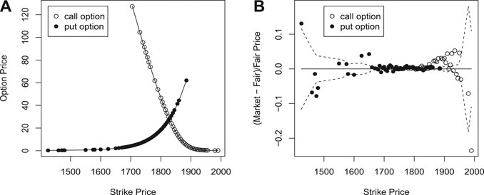
FIGURE 1. Leave-one-out cross-validation for options traded on April 14, 2014 with an expiration date of September 5, 2014 (round dot: market price; solid line: fair price based on PC; dash line: 95% confidence interval based on bootstrap).

To have a closer look at the difference between market price and fair price, we plot the relative difference, that is (market price - fair price)/fair price, against strike price in Figure 1B. The sign of the relative difference tells us whether the option is under- or overpriced. In addition, in order to check if the difference between a market price and its fair price is statistically significant, we bootstrap the rest of the market prices 50 times to obtain a 95% confidence interval of the fair price. The dash lines in Figure 1B show the upper and lower ends of the bootstrap confidence intervals. When a market price falls outside its bootstrap confidence interval, we may report to investors that the corresponding option is significantly under-/overpriced compared with the market prices of the other options.

4 Pricing Variance Swap

With an estimated RND, one can calculate the fair price of any derivative whose payoff is a function of $S_T$. In this section, we apply the proposed method to price variance swaps. Our study shows that our fair prices match the market prices of long-term variance swaps reasonably well.

A variance swap is a financial product that allows investors to trade realized variance against current implied variance of log returns. More specifically, let $S_t$ stand for the closing price of the underlying asset on day t, $t=\mathrm{0,1},\dots ,T$, and let $R_t=\text{log}\left(S_t/S_{t-1}\right)$ represent the tth daily log return. The annualized realized variance over T trading days is defined as ${\sigma }_{\text{realized}}^2=\frac{A}{T}{{\displaystyle \sum }}_{t=1}^T{R}_t^2$, where A is the number of trading days per year, which on average is 252. The payoff of a variance swap is defined as

$N_{\text{var}}\left({\sigma }_{\text{realized}}^2-{\sigma }_{\text{strike}}^2\right),$

where the variance notional $N_{\text{var}}$ and variance strike ${\sigma }_{\text{strike}}^2$ are specified before the sale of a variance swap contract.

Variance swaps provide investors with pure exposure to the variance of the underlying asset without directional risk. It is notably liquid across major equities, indices, and stock markets and is growing across other markets. Historical evidence indicates that selling variance is systematically profitable.

There are numerous methods in the literature of pricing variance swaps, both analytically and numerically (see [13] for an extensive review). Nevertheless, a pricing formula or procedure that relies on a certain stochastic process, for instance, Lévy process [14], MRG-Vasicek model [17], or Hawkes jump-diffusion model [18], may suffer from a lack of parsimony or might not fit the real data well due to the inappropriateness of model assumptions (see, for instance, [14]).

In this section, we propose a moment-based method in conjunction with our PC RND estimate to price variance swaps, which is free of model assumption.

Assuming the existence of a risk-neutral measure $\mathbb{Q}$, the fair price $V{S}_{t,T}$ of a variance swap on day t is the discounted expected payoff:

$V{S}_{t,T}=e^{-R_{tT}}{N}_{\text{var}}\left[{\mathbb{E}}_t^{\mathbb{Q}}\left(\frac{A}{T}{\displaystyle \sum }_{i=1}^T{R}_i^2\right)-{\sigma }_{\text{strike}}^2\right],(11)$

where $R_{tT}$ is the cumulative risk-free interest rate from t to T defined in The Proposed Piecewise Constant Nonparametric Approach. To proceed, we further assume the following.

Assumption 1. The increments of the process $\text{log}{S}_t$ are independent; that is, $\text{log}\left(S_{t+1}/S_t\right)$ is independent of $S_0,\dots ,S_t$, $t=0,\dots ,T-1$.

Consequently, the fair price of a variance swap can be represented by a sequence of the risk-neutral moments of the underlying asset.

Proposition 4.1. Assuming the existence of a risk-neutral measure $\mathbb{Q}$ and that Assumption 1 is fulfilled, the fair price of variance swap is

$V{S}_{t,T}=e^{-R_{tT}}{N}_{\text{var}}\left\{\frac{A}{T}\stackrel{t}{{\displaystyle \sum }_{i=1}}{R}_i^2+\frac{A}{T}{\mathbb{E}}_t^{\mathbb{Q}}{\left(\log S_T\right)}^2-\frac{A}{T}{\left(\log S_t\right)}^2-\frac{2A}{T}\stackrel{T}{{\displaystyle \sum }_{i=t+1}}\left[{\mathbb{E}}_t^{\mathbb{Q}}\log S_{i-1}{\mathbb{E}}_t^{\mathbb{Q}}\log S_i-{\left({\mathbb{E}}_t^{\mathbb{Q}}\log S_{i-1}\right)}^2\right]-{\sigma }_{\text{strike}}^2\right\}.(12)$

The proof of Proposition 4.1 is relegated to Supplementary Material C.

4.1 Moments Calculation

In view of Eq. 12, pricing variance swaps requires estimating the first and second moments of $\text{log}{S}_i$ under the risk-neutral measure. One option is to use a moment-based method described by [16] and further extended by [19]. In this section, we employ an alternative way of calculating the moments, which makes use of the proposed nonparametric approach.

Recall that the step function $f_{\text{Δ}}$ defined in Eq. 1 or Eq. 10 provides an approximation to the RND $f_{\mathbb{Q}}$ of $\text{log}{S}_T$ . We use all the available market prices of options to estimate $f_{\text{Δ}}$; then, the moments calculated from $f_{\text{Δ}}$ serve as the estimates of required moments. Since $f_{\text{Δ}}$ is “PC” which stands for piecewise constant. it can be verified that the first and second moments of $\text{log}\left(S_T\right)$ are given by

${\mathbb{E}}_t^{\mathbb{Q}}\text{log}\left(S_T\right)=\stackrel{q+1}{{\displaystyle \sum }_{l=1}}\frac{a_l}{2}\left[{\left(\log K_l\right)}^2-{\left(\log K_{l-1}\right)}^2\right],(13)$

${\mathbb{E}}_t^{\mathbb{Q}}{\left[\text{log}\left(S_T\right)\right]}^2=\stackrel{q+1}{{\displaystyle \sum }_{l=1}}\frac{a_l}{3}\left[{\left(\log K_l\right)}^3-{\left(\log K_{l-1}\right)}^3\right].(14)$

Note that there are no market prices available for options that expire on a day that is other than the third Saturday of the delivery month. We would have to interpolate the mean and standard deviation of $\text{log}\left(S_i\right)$ for $t<i<T$, and this is achieved via linear interpolation in this paper. Detailed procedures are described in Supplementary Material D.

4.2 Replicating by Variance Futures

In order to evaluate the fair price of a variance swap, we replicate variance swap using available market prices of variance futures. Variance future is a financial contract that is traded over the counter. As stated in [20], variance swap and variance future are essentially the same since they both trade the difference of variance and one can replicate a variance swap by the corresponding variance future. As a matter of fact, if variance future and variance swap share the same expiration date, then at the start point of the observation period, there is no difference between trading a variance future and trading a variance swap with $50 variance notional. The formula for the fair price of a variance swap contract induced from variance future is given by

$V{S}_{t,T}=e^{-R_{tT}}{N}_{\text{var}}\left\{\frac{A}{T}\left[{\displaystyle \sum }_{i=1}^{M-1}{R}_i^2+IUG\times \frac{N_e-M+1}{A}\times \frac{1}{{100}^2}\right]-{\sigma }_{\text{strike}}^2\right\},$

where M is the number of observed days to date, $N_e$ is the expected number of trading days in the observation period, and $IUG$ is the square of market implied volatility given by

$IUG={\displaystyle \sum }_{i=M}^{N_e}{R}_i^2\times \frac{A}{N_e-M+1}\times {100}^2.$

4.3 Variance Future Data

Variance future data were downloaded from the Chicago Board Options Exchange (CBOE) website (http://cfe.cboe.com/). Variance future products with 12-month (with futures symbol VA) or 3-month (with futures symbol VT) expirations are traded on the CBOE Futures Exchange. We use VA in the subsequent analysis. The continuously compounded zero-coupon interest rates cover dates from January 2, 1996 to August 31, 2015. For variance futures, the trading dates are from December 10, 2012, to August 31, 2015, with start dates from December 21, 2010, to July 30, 2015, and expiration dates from January 18, 2013, to January 1, 2016. We use variance futures to replicate variance swaps, so the time spans of variance swaps are in line with those of variance futures.

4.4 Results

In order to assess the accuracy of our estimated fair prices of a variance swap, we compare three relevant quantities:

1. OP: Fair price of a variance swap based on our moment-based nonparametric approach, using option market prices till day t

2. VF: Induced market price of a variance swap from CBOE traded variance future till day t

3. True: Realized price of a variance swap at expiration day T with known $S_0,S_1,\dots ,S_T$

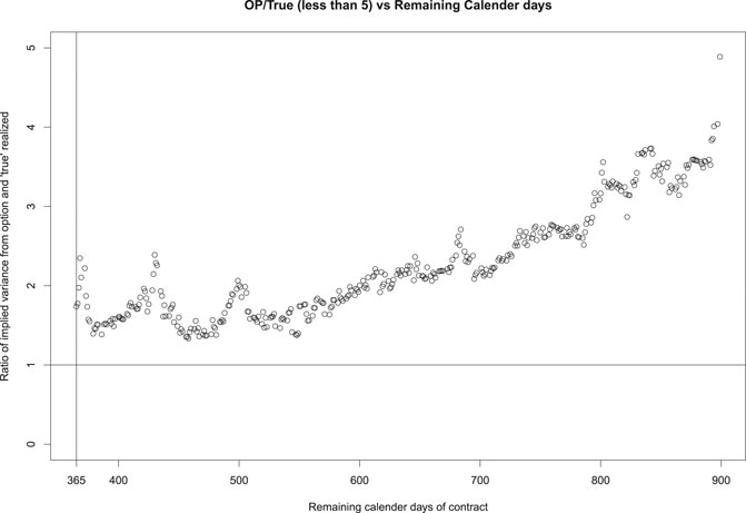
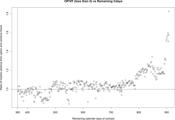
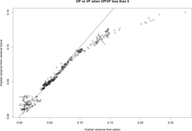
We present three ratios, OP/True, VF/True, and OP/VF, in Figures 2–4, respectively, against the remaining calendar days of variance swaps. Compared with ‘True’ prices based on realized underlying asset prices, Figure 2 and Figure 3 suggest that OP and VF have a similar increasing pattern along with the remaining calendar days. This is in part due to the uncertainty in the estimate of the variance, which increases with the number of days to expiration. On the other hand, Figure 4 and Figure 5 show that the fair price OP based on our proposed method matches the market price VF pretty well on variance swaps with expiration between 365 and 800 days. For variance swaps expiring in less than 365 days (not shown here), OP and VF do not match well. This is plausibly attributed to the fact that long-term options are more reasonable and stable, which are less likely to be affected by external factors or noises. For variance swaps longer than 800 days, the relatively low VF might indicate underpriced variance futures.

FIGURE 2

FIGURE 2. Ratio of OP/True variance swap prices vs. days to expiration.

FIGURE 3

FIGURE 3. Ratio of VF/True variance swap prices vs. days to expiration.

FIGURE 4

FIGURE 4. Ratio of OP/VF variance swap prices vs. days to expiration.

FIGURE 5

FIGURE 5. OP vs. VF variance swap prices.

5 Discussion

In this article, we propose a new nonparametric approach for estimating the RND. It is data-driven and is not built on any model assumption about the data generating process of underlying asset prices. It only assumes the existence of an RND and the independence of increments of log return for pricing variance swaps. That is why it can capture the market price very well.

In contrast with other nonparametric methods, such as cubic spline and B-spline, our method is much simpler but fits the real data better. We choose only distinct strikes as knots and assume constant values between knots to avoid overfitting. By sacrificing the continuity of estimated RND, the nonnegativity of a density function is readily satisfied.

On the other hand, the proposed approach utilizes market prices of all options, not just OTM options. In our opinion, ITM options, despite not being as liquid as OTM options, still contain market information and should be incorporated when estimating a RND. Our comprehensive analysis shows that it recovers OTM option prices better by including ITM option prices.

One of the potential applications of our work is to price OTC securities. The comprehensive comparisons of different methods using S&P 500 European option data in Pricing European Options show the outperformance of our estimates across various time-to-maturity periods. With our estimated RNDs, financial engineers may be able to develop more sophisticated financial products to fit the needs of their customers better. A fair price of the new financial product will not only facilitate the traders but also reduce their financial risk.

Another potential application is to build up profitable portfolios for investment purposes. In Detecting Profitable Opportunities, we show how to use leave-one-out and bootstrap techniques to identify under- or overpriced options from fair-priced options. Real-time trading algorithms may be developed based on our estimates toward catching up profitable opportunities by buying underpriced options and shorting overpriced options.

Pricing variance swaps is a difficult job when dealing with real data. We display in Figures 2–5 only the cases where the ratio OP/True is less than 5. There are cases where OP and VF disagree significantly. Overall, our OP prices work better for variance futures that expire in the last four months of 2015, which are also the last four months available in our dataset.

In the literature, RND is naturally connected to the concept of statistic discount factor or pricing kernel, which can be described as the ratio of the RND and the physical density [21]. The proposed nonparametric estimate of RND could be applied to estimate pricing kernel as well.

Data Availability Statement

Publicly available datasets were analyzed in this study. This data can be found here: http://cfe.cboe.com/, Chicago Board Options Exchange (CBOE) website.

Author Contributions

LJ and SZ processed the experimental data and performed the analysis. LJ drafted the manuscript. JY, LJ, and KL developed the theory and performed the analytical calculations. FW and KL helped supervise the project. JY, FW, and LJ conceived the original idea. JY supervised the project. All authors discussed the results and contributed to the final manuscript.

Conflict of Interest

The authors declare that the research was conducted in the absence of any commercial or financial relationships that could be construed as a potential conflict of interest.

Acknowledgments

We thank Liming Feng from the University of Illinois at Urbana-Champaign and Yuhang Liang from Northwestern University for their enormous help during data collection.

Supplementary Material

The Supplementary Material for this article can be found online at: https://www.frontiersin.org/articles/10.3389/fams.2020.611878/full#supplementary-material.

References

1. Malz, AM. A simple and reliable way to compute option-based risk-neutral distributions. In: Staff report New York, NY: Federal Reserve Bank of New York. (2014). p 677.

2. Melick, W, and Thomas, C. Recovering an asset’s implied pdf from option prices: an application to crude oil during the gulf crisis. J Financ Quant Anal (1997). 32:91–115. doi:10.2307/2331318

CrossRef Full Text | Google Scholar

3. Taboga, M. Option-implied probability distributions: how reliable? How jagged? Int Rev Econ Finance (2016). 45:453–69. doi:10.1016/j.iref.2016.07.013

CrossRef Full Text | Google Scholar

4. Breeden, D, and Litzenberger, R. Prices of state-contingent claims implicit in option prices. J Bus (1978). 51:621–51.

CrossRef Full Text | Google Scholar

5. Bliss, R, and Panigirtzoglou, N. Testing the stability of implied probability density functions. J Bank Finance (2002). 26:381–422. doi:10.2139/ssrn.209650

CrossRef Full Text | Google Scholar

6. Jarrow, R, and Rudd, A. Approximate option valuation for arbitrary stochastic process. J Financ Econ (1982). 10:347–69. doi:10.1016/0304-405X(82)90007-1

CrossRef Full Text | Google Scholar

7. Ritchey, R. Call option valuation for discrete normal mixtures. J Financ Res (1990). 13:285–96. doi:10.1111/j.1475-6803.1990.tb00633.x

CrossRef Full Text | Google Scholar

8. Sherrick, B, Irwin, S, and Forster, D. Option-based evidence of the nonstationarity of expected SP 500 futures price distributions. J Futures Mark (1992). 12:275–90. doi:10.1002/fut.3990120304

CrossRef Full Text | Google Scholar

9. Eriksson, A, Ghysels, E, and Wang, F. The normal inverse Gaussian distribution and the pricing of derivatives. J Deriv (2009). 16:23–37. doi:10.3905/JOD.2009.16.3.023

CrossRef Full Text | Google Scholar

10. Ghysels, E, and Wang, F. Moment-implied densities: properties and applications. J Bus Econ Stat (2014). 32:88–111. doi:10.1080/07350015.2013.847842

CrossRef Full Text | Google Scholar

11. Monteiro, A, Tutuncu, R, and Vicente, L. Recovering risk-neutral probability density functions from options prices using cubic splines. Eur J Oper Res (2008). 187:525–42. doi:10.1016/j.ejor.2007.02.041

CrossRef Full Text | Google Scholar

12. Lee, S. Estimation of risk-neutral measures using quartic b-spline cumulative distribution functions with power tails. Quant Finance (2014). 14:1857–79. doi:10.1080/14697688.2012.742202

CrossRef Full Text | Google Scholar

13. Zhu, SP, and Lian, GH. A closed-form exact solution for pricing variance swaps with stochastic volatility. Math Finance (2010). 21:233–56. doi:10.1111/j.1467-9965.2010.00436.x

CrossRef Full Text | Google Scholar

14. Carr, P, Lee, R, and Wu, L. Variance swaps on time-changed Lévy processes. Finance Stochast (2012). 16:335–55. doi:10.1007/s00780-011-0157-9

CrossRef Full Text | Google Scholar

15. Eriksson, A, Ghysels, E, and Forsberg, L. Approximating the probability distribution of functions of random variables: a new approach. Montreal, Canada:Cirano (2004). p 503.

16. Bakshi, G, Kapadia, N, and Madan, D. Stock return characteristics, skew laws, and the differential pricing of individual equity options. Rev Financ Stud (2003). 16:101–43. doi:10.2139/srn.282451

CrossRef Full Text | Google Scholar

17. Han, Y, and Zhao, L. A closed-form pricing formula for variance swaps under MRG-Vasicek model. Comput Appl Math (2019). 38:142. doi:10.1007/s40314-019-0905-6

CrossRef Full Text | Google Scholar

18. Liu, W, and Zhu, SP. Pricing variance swaps under the Hawkes jump-diffusion process. J Futures Mark (2019). 39:635–55. doi:10.1002/fut.21997

CrossRef Full Text | Google Scholar

19. Rompolis, LS, and Tzavalis, E. Retrieving risk neutral moments and expected quadratic variation from option prices. Rev Quant Finance Account (2017). 48:955–1002. doi:10.2139/ssrn.936670

CrossRef Full Text | Google Scholar

20. Biscamp, L, and Weithers, T. Variance swaps and cboe s and p 500 variance futures. Chicago Trading Company, LLC. (2007). p 25.

Google Scholar

21. Beare, BK, and Schmidt, LD. An empirical test of pricing kernel monotonicity. J Appl Econom (2016). 31:338–56. doi:10.1002/jae.2422

CrossRef Full Text | Google Scholar