 David Medina
 Pablo Padilla
95% of researchers rate our articles as excellent or good
Learn more about the work of our research integrity team to safeguard the quality of each article we publish.
Find out more
ORIGINAL RESEARCH article
Front. Appl. Math. Stat. , 17 June 2020
Sec. Statistical and Computational Physics
Volume 6 - 2020 | https://doi.org/10.3389/fams.2020.00020
This article is part of the Research Topic Analytical and Numerical Methods for Differential Equations and Applications View all 11 articles
In this paper we study the attractor of a parabolic semiflow generated by a singularly perturbed PDE with a non-linear term given by a bistable potential, in an oval surface; the Allen-Cahn equation being a prototypical example. An additional constraint motivated by a variational principle for closed geodesics originally proposed by Poincaré arising from geometric considerations is introduced. The existence of a global attractor is established by modifying standard techniques in order to handle the constraint. Based on previous work on the elliptic case, it is known that when the perturbation parameter tends to zero, minimal energy solutions exhibit a sharp interface concentrated on a closed geodesic. We provide numerical simulations using Galerkin's method. Based on the analytical and numerical results we conjecture that, when the perturbation parameter tends to zero and for large times, the transition layers of the solutions of this PDE consists of closed geodesics or a union of arcs of such geodesics, thus characterizing the structure of the attractor.
The qualitative study of dynamical systems in infinite dimensions has been of fundamental importance. In the case of dynamical systems associated with partial differential equations of evolution having variational structure, many of the ideas and methodologies of gradient-like systems can be extended to infinite dimensions. In particular, the study and characterization of attractors is of special interest.
In this paper, we prove the existence of the global attractor of the parabolic equation associated to:
on an oval surface M1 (see Figure 1) where u : M → ℝ, 0 < ϵ ≪ 1, Δ represents the Laplace–Beltrami operator on M and W(u) is a non-linear term, which in particular includes the Allen-Cahn non-linearity. The flow will be considered in a space of functions satisfying a geometric constraint to be explained later.
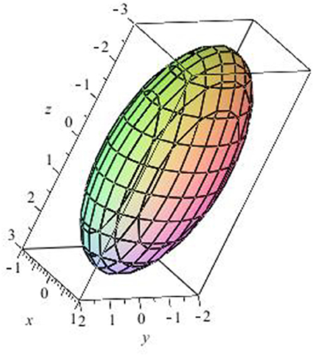
Figure 1. Example of an oval surface in ℝ3.
Equation (1) arises in many contexts among which we may mention materials science, superconductivity, population dynamics, and pattern formation.
An important case for W(u) is given by W(u) = (1 − u2)2, which has been widely studied both analytically and numerically for example in Hutchinson and Tonewaga [1] and Padilla and Tonewaga [2] and references therein.
In a bounded domain Ω ⊂ ℝn, n ≥ 2, with suitable initial and boundary conditions, in Bronsard and Kohn [3], it is shown that, when ϵ → 0, the solution u of (1) separates Ω in two regions where u ≈ 1 and u ≈ −1, respectively, and the transition layer, moves with normal velocity equal to its principal curvatures. A similar behavior occurs on an oval surface for non-trivial solutions of (1). Using results in Hutchinson and Tonewaga [1] and Padilla and Tonewaga [2], in Garza-Hume and Padilla [4] it is established that, when ϵ → 0, non-trivial minima of the corresponding energy function (with a suitable restriction) have a transition layer located at the shortest closed geodesic.
This fact is obtained using the variational structure of the problem, because (1) is the Euler Lagrange equation of the functional:
in a suitable functional space.
For ϵ → 0, functions u with uniformly bounded energy Eϵ(u) < E0, can be proved to be close to ±1 in most of the domain, except for a transition curve. The proof follows from a classical result in differential geometry due to Birkhoff that guarantees the existence of a closed geodesic on a surface diffeomorphic to the sphere (see Poincaré [5] where the corresponding variational principle was first conjectured, later demostrated by Berger and Bombieri [6]):
Proposition 1. Suppose that γ is a closed curve on M that under the Gauss map, g, divides the unit sphere in two parts of equal measure. Assume further that among all the curves satisfying the above conditions, γ has minimal length. Then γ is a closed geodesic.
This fact suggests a natural constraint for the problem under consideration. The function u belongs to the space of functions that satisfies:
where g is the Gauss map.
On the other hand, solutions of (1) correspond to stationary points of the associated gradient flow:
The main goal of this paper is show the existence of the attractor of the associated parabolic equation to (1) (i.e., Equation 4), and conjecture its structure in terms of functions that possess transition layers determined by closed geodesics or arcs of geodesics. In other words, given any initial condition, the corresponding parabolic semiflow determined by (4) approaches a function with transitions in geodesics. This will be done by considering the special case in which M = S2 and W(u) = (1 − u2)2. This will simplify both the analysis and the numerics.
From now on we consider solutions of (4) satisfying the constraint (3). Under the above restrictions, it becomes:
which will be incorporated into the equation later on as a Lagrange multiplier. As a first step, we will proof the existence of an attractor for (4) under the constraint (5). We will recall some standard facts in dynamical systems theory, Sobolev spaces on Riemannian manifolds as well as Gronwall's inequality, which are presented in the following section. This is done for the sake of completeness and to introduce notation and may be skipped by readers familiar with dynamical systems and analysis on manifolds.
Having shown the existence of the attractor, some numerical experiments are performed using the Galerkin method. A few words are in order regarding the limitations of our numerical approach. Even when in principle the method should be applicable for any initial condition, we only considered some that already exhibit a relatively well-defined interface. The aim of the numerical simulations is to make plausible our conjecture on the structure of the global attractor and a more detailed study of the method is not carried out. As for the analytical approach, we remark that the problem of establishing the existence of a global attractor for other surfaces or manifolds in similar situations seems to be a reasonable extension of the methods and ideas here presented. In particular for the case of surfaces with non-zero Euler characteristic as is done in Del Río et al. [14] for the elliptic case.
The notation and terminology used in this section is adapted or quoted from Temam [7], although arguments and results in Sell and You [8] and Robinson [9] are also used. Since these are standard results and references, no explicit references are made.
We will consider dynamical systems whose state is described by an element u(t) of a metric space H. In most cases, and in particular for dynamical systems associated with partial or ordinary differential equations, the parameter t (the time or the timelike variable) varies continuously in ℝ or in some interval of ℝ. Usually the space H will be a Hilbert or Banach space.
The evolution of the dynamical system is described by a family of operators S(t), t ≥ 0, that map H into itself and enjoy the usual semigroup properties:
If ϕ is the state of the dynamical system at time s, then S(t)ϕ is the state of the system at time t + s, and
The semigroup S(t) will be determined in our case by the solution of a PDE. The basic properties of the operators S(t) which are needed will be established in the next subsection but, for the time being, we assume that:
These operators may or may not be one-to-one; the injectivity property is equivalent to the backward uniqueness property for the dynamical system. When S(t), t > 0, is one-to-one we denote by S(−t) its inverse which maps S(t)H onto H; we then obtain a family of operators S(t), t ∈ ℝ, which have the property (6) on their domains of definition, ∀s, t ∈ ℝ. It is clear that for t < 0, the operators S(t), are not usually defined everywhere in H.
Definition 1. For u0 ∈ H the orbit or trajectory starting in u0 is the set ⋃t ≥ 0S(t)u0.
Definition 2. When it exists, an orbit or trajectory ending at u0 is the set .
Definition 3. For u0 ∈ H or for , the ω-limit set of u0 (or ) is
or
where closures are taken in H.
Definition 4. When it exists, the α-limit set of u0 ∈ H or is
or
Proposition 2. if and only if there exists a sequence of elements of and a sequence tn → ∞ such that
Remark 1. Analogously, if and only if there exists a sequence ψn converging to ψ in H and a sequence tn → ∞, such that .
Definition 5. A fixed point, or an equilibrium point is a point u0 ∈ H such that
We say that a set X ⊂ H is positively invariant for the semigroup {S(t)}t ≥ 0 if
It is said to be negatively invariant if {S(t)}t ≥ 0 if
When the set is both positively and negatively invariant, we call it an invariant set or a functional invariant set.
Definition 6. A set X ⊂ H is a invariant set for the semigroup {S(t)}t ≥ 0 if
The simplest examples of invariant sets are equilibrium points, heteroclinic orbits and limit cycles.
Lemma 1. Assume that for some subset , and for some t0 > 0, the set is relatively compact in H. Then is non-empty, compact, and invariant.
Definition 7. An attractor is a set that enjoys the following properties:
1. is an invariant set.
2. possesses an open neighborhood such that, for every , S(t)u0 converges to as t → ∞. This means that:
as t → ∞.
The distance in (2) is understood to be the distance of a point to a set:
d(x, y) denoting the distance of x to y in H.
Definition 8. If is an attractor, the largest open set that satisfies (2) is called the basin of attraction of . Alternatively, we say that attracts the points of .
Definition 9. It is said that uniformly attracts a set if
as t → ∞.
is now the semidistance of two sets:
The convergence in the above definition is equivalent to the following: for every ϵ > 0, there exists tϵ such that for is included in , the ϵ-neighborhood of . When no confusion can occur we simply say that attracts .
Definition 10. We say that is a global (or universal) attractor for the semigroup {S(t)}t ≥ 0 if is a compact attractor that attracts the bounded sets of H (and its basin of attraction is then all of H).
It is easy to see that such a set is necessarily unique. Also such a set is maximal for the inclusion relation among the bounded attractors and among the bounded functional invariant sets. For this reason it is also called the maximal attractor.
In order to establish the existence of attractors, a useful concept is the related concept of absorbing sets.
Definition 11. Let be a subset of H and an open set containing . We say that is absorbing in if the orbit of any bounded set of enters after a certain time (which may depend on the set):
We say also that absorbs the bounded sets of .
The existence of global attractor for a semigroup {S(t)}t ≥ 0 implies that of an absorbing set. Indeed, for ϵ > 0, let denote the ϵ-neighborhood of (i.e., the union of open balls of radius ϵ centered on ). Then, for any bounded set as t → ∞; hence for t ≥ t(ϵ) and for such t's. This shows that is an absorbing set.
Conversely, it is a standard result that a semigroup that possesses an absorbing set and enjoys some other properties possesses an attractor.
In order to prove existence of an attractor when the existence of an absorbing set is known, we need further assumptions on the semigroup {S(t)}t ≥ 0, and we will make one of the two following:
• The operators S(t) are uniformly compact for t large. By this we mean that for every bounded set there exists t0 which may depend on such that
is relatively compact in H.
Alternatively, if H is a Banach space, we may assume that S(t) is the perturbation of an operator satisfying (11) by a (non-necessarily linear) operator which converges to 0 as t → ∞. More precisely:
• If H is a Banach space and for every t, S(t) = S1(t) + S2(t) where the operators S1(·) are uniformly compact for t large and S2(t) is a continuous mapping from H into itself such that the following holds:
For every bounded set C ⊂ H,
as t → ∞.
Of course, if H is a Banach space, any family of operator satisfying (11) also satisfies (12) with S2 = 0.
Theorem 1. Assume that H is a metric space and that the operators S(t) are given and satisfying (6), (9) and either (11) or (12). We also assume that there exists an open set and a bounded set of such that is absorbing in .
Then the ω-limit set of , is a compact attractor which attracts the bounded sets of . It is the maximal bounded attractor in (for the inclusion relation).
Furthermore, if H is a Banach space, if is convex, and the mapping t ↦ S(t)u0 is continuous from ℝ+ into H, for every u0 in H; then is connected too.
The proof of this theorem is carried out through several steps, which can be found in Temam [7].
The notation and terminology used in this section can be found in Hebey [11] and Aubin [12].
Let (M, g) be a smooth Riemannian manifold. Given k an integer, and p ≥ 1 real, set
When M is compact, one clearly has that for any k and any p ≥ 1. For , set also
We define the Sobolev space as follows:
Definition 12. Given (M, g) a smooth Riemannian manifold, k an integer, and p ≥ 1 real, the Sobolev space is the completion of with respect to .
Note here that one can look at these spaces as subspaces of Lp(M), in which the norm of is defined by
Definition 13. Given (E, ||·||E) and (F, ||·||F) two normed vector spaces with the property that E is a subspace of F, we say that the embedding of E in F is compact if bounded subsets of (E, ||·||E) are relatively compact in (F, ||·||F). This fact is written as E ⊂ ⊂ F.
This means that bounded sequences in (E, ||·||E) possess corvergent subsequences in (F, ||·||F). Clearly, if the embedding of E in F is compact, it is also continuous, i.e., if there exists C > 0 such that for any x ∈ E, ||x||F ≤ C||x||E.
The following theorem is needed in order to prove the existence of the attractor of the equation in consideration.
Theorem 2. Let (M, g) be a smooth, compact Riemannian n-manifold. For any real numbers 1 ≤ q < p and any integers 0 ≥ m < k, if 1/p = 1/q − (k − m)/n, then . In particular, for any q ∈ [1, n), where 1/p = 1/q − 1/n.
The first part of the above theorem has the following consequence:
Corollary 1. For any q ∈ [1, n), , thus for all p ≥ 1.
The following inequality is derived from Gronwall's lemma and will be used later on.
Lemma 2. Let y a positive absolutely continuous function on (0, ∞) which satisfies:
with p > 1, γ > 0, δ ≥ 0. Then, for t > 0,
Proof: If y(0) ≤ (γ/δ)1/p, then y(t) ≤ (γ/δ)1/p, ∀t ≥ 0. If y(t) > (γ/δ)1/p, then there exists t0 ∈ (0, ∞) such that y(t) ≥ (γ/δ)1/p for 0 ≤ t ≤ t0, and y(t) ≤ (γ/δ)1/p for t ≥ t0.
For t ∈ [0, t0] we write z(t) = y(t) − (γ/δ)1/p ≥ 0 and since (a + b)p ≥ ap + bp for a, b ≥ 0, p > 1, we have
Hence
and then by integration
This implies the desired result for t ∈ [0, t0], and since, this inequality holds for t ≥ t0, the lemma is proved.
The main result is the following in which the existence of a global attractor is shown for equation (4) subject to constraint (5).
Theorem 3. The semigroup {S(t)}t ≥ 0 associated with (4) - (5) possesses a maximal attractor which is bounded in , compact and connected in L2(S2). Its basin of attraction is the whole space L2(S2), and attracts bounded sets of L2(S2).
Proof: The existence of a solution proposed equation is equivalent to finding the minimum of:
for all , subject to the constraint:
where f(y) is the Jacobian determinant of the transformation of S2 into M. This determinant can be considered to be positive, and this factor is the Gaussian curvature in y.
For fixed ϵ > 0, the existence of this minimum is a consequence of this functional satisfies the Palais–Smale condition (see Struwe [13]), is bounded below and the constraint defines a closed lineal subspace.
On other hand it should be noted that:
This last statement ensures the existence of a global solution for t > 0. This is sufficient to define the associated semiflow to given equation.
Another way to verify the above statement, is to first prove the existence and uniqueness of a solution of (4)–(5) subject to a suitable initial condition; then the backward uniqueness in order to show existence for all t ∈ ℝ. Finally apply the theorem 4 for the characterization of global attractor.
In the usual way, we shall see the existence of an absorbent set in L2(S2) and subsequently, the compactness of the mentioned semigroup, according to theorem 1.
The Euler–Lagrange equation associated to (2) with the constraint (3) (for each ϵi), contain a Lagrange multiplier λi as follows:
In Del Río et al. [14], it is shown that these multipliers are bounded. This fact will be used later.
In order to prove the existence of an absorbing set in L2(S2), we multiply (2) by u and integrate over S2. Using Green's formula we obtain:
where denotes the norm L2(S2).
By a standard corollary (see for instance 1) , therefore there exists a constant c0 such that , and there exists a c1 such that:
An estimate of the third integral in (15) is required, for which the following inequality is used:
and by Hölder's inequality, for a C > 0:
and for certain A, B > 0:
Thanks to (15) and the previous relationship, we conclude that there exists a such that:
Thus:
this meaning that:
According to (16) concluded from (17), there exists a such that:
By using the classical Gronwall lemma, we obtain that:
Therefore:
There exists an absorbing set in L2(S2), namely, any ball of L2(S2) centered at 0 of radius R > ρ0, as if is a bounded set of L2(S2), included in a ball B(0, R) of L2(S2), then for , with
In order to prove the uniform compactness of operators, we proceed using by an argument proposed by B. Nicolaenko (see Temam [7]) and making use of the absorbent set in L2(S2) whose existence was established in the previous paragraph.
By Holder inequality:
Analogously to (15), we conclude that:
where . Lemma 2 shows that:
Let ρ2 be a real number greater than (γ/δ)1/2 and
The above relations show that for any set of L2(S2), bounded or not, is included in the ball centered at 0 of radius ρ2, if t ≥ T0, thus demostrating the existence of an absorbent set in . The uniform compactness of operators S(t) follows from the fact that a bounded set is included in a ball B(0, R) for all t ≥ t0, that which is bounded in and relatively compact in L2(S2) (corollary 1). The existence of the global attractor follows from theorem 1.
Having shown the existence of a global attractor, the question of characterizing its structure arises. This question can be answered provided there is a suitable Lyapunov functional.
Definition 14. A Liapunov functional for {S(t)}t ≥ 0 on a set is a continuous function such that:
1. For each , the function t → F(S(t)u0) is non-increasing.
2. If F(S(τ)u1) = F(u1) for some τ > 0, then u1 is a fixed point of {S(t)}t ≥ 0, i.e., S(t)u1 = u1, ∀t > 0.
The following standard theorem establishes the structure of the attractor.
Theorem 4. Let there be a given semigroup {S(t)}t ≥ 0 which enjoys the properties (6), (7). We assume that there exists a Lyapunov functional as in the definition 14, and a global attractor . Let denote the set of fixed points of the semigroup. Then
Furthermore, if is discrete, is the union of and of the heteroclinic curves joining points of and
Remember that, is the set (maybe empty) of points u*, which belongs to an orbit {u(t), t ∈ ℝ} such that d(u(t), X) → 0 as t → ∞.
The details of this proof can be found in Temam [7] theorem 4.1 in chapter 7, Robinson [9] theorem 10.13, Ladyzhenskaya [17] theorem 3.2, or Sell [8] theorem 72.1.
Once the existence of an attractor is proved, in this section we provide a numerical method for its characterization. In this implementation the Galerkin method is used.
S2 is parametrized with spherical coordinates by (r cos θ cos ϕ, r sin θ cos ϕ, r sin ϕ), where 0 ≤ θ ≤ 2π y (see Figure 2).
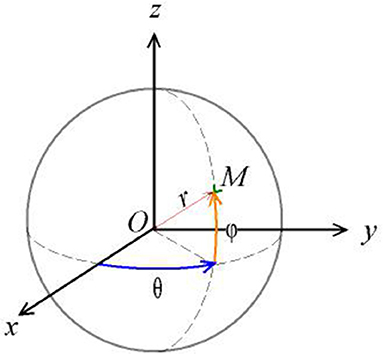
Figure 2. Spherical coordinates using longitude θ and latitude ϕ.
Then, the Laplacian in these coordinates is given by:
Using r = 1 in the above expression, the Laplace–Beltrami operator in S2 is obtained:
Then (4) becomes:
By implementing Galerkin's method, we can approximate the attractor. This is done by projecting Equation (18), with a suitable initial condition on a finite dimensional subspace, thus reducing it to a system of ordinary differential equations. The details are provided in the next section.
The idea is to obtain a finite dimensional reduction of (18). One way to do this is using Galerkin method, which will be described below (for more details see Kythe et al. [15] and Evans [10]).
We consider the problem:
Assume that the funtions wk = wk(θ, ϕ), (k = 1, …) are smooth, is an orthogonal basis of and an orthonormal basis of L2(S2). For instance, we could take to be the complete set of eigenfunctions of Δ in S2.
Fix now a positive integer m. We will look for an approximation um of the form
where we will select the coefficients so that:
and
Here (·, ·) denotes the inner product in L2(S2), is the bilinear form:
and
Thus, we look for a function um of the form (21) that satisfies the projection (23) of problem (19)–(20) onto the finite dimensional subspace spanned by .
By the standard theorem on existence and uniqueness of systems of ordinary differential equations, we have the following result:
Theorem 5. For each integer m = 1, 2, …, there exists a unique funtion um of the form (21) satisfying (22), (23).
Functions wk, will be selected via the method of separation of variables, applied to the equation Δu = 0 on S2, i.e., we assume that u = Θ(θ)Φ(ϕ), where we have:
The corresponding solutions for Θ are of the form sine and cosine, while those corresponding to Φ are solutions to the Legendre equation, in which the substitution x = sin ϕ has been made. Thus, we use the associated Legendre polynomial denoted by P(k, l, x), which is defined by:
where k ≥ 0 and l ≤ k. (For more details see Arfken [16]).
According to the above condition (5) we choose the functions um as:
with m = 1 and ϵ = 0.001, (23) becomes:
If the initial condition (22) is
we obtain
and
Figure 3 show the behavior of u1 at different times (t = 0, t = 0.0001, t = 1).
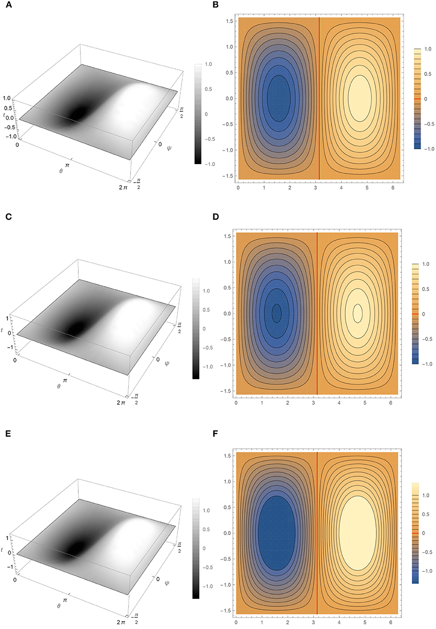
Figure 3. Behavior of u1(t) for different values of t according to Equation (29). (A) Graph of u1(0). (B) Level curves of u1(0). (C) Graph of u1(0.001). (D) Level curves of u1(0.001). (E) Graph of u1(1). (F) Level curves of u1(1).
If the initial condition is now,
then
and
Figure 4 show the behavior of u1 at different times (t = 0, t = 0.01, t = 0.02).
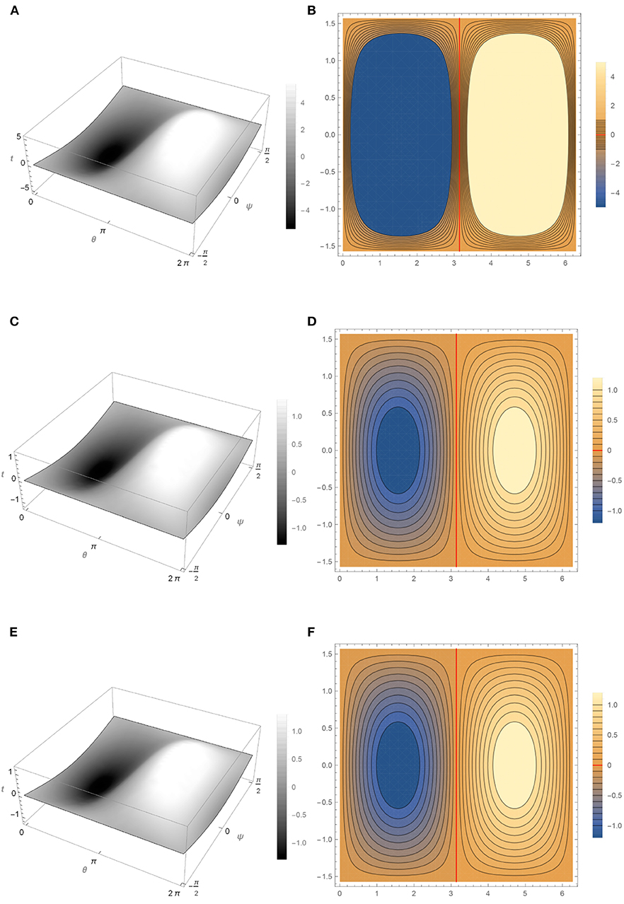
Figure 4. Behavior of u1(t) for different values of t according to Equation (29). (A) Graph of u1(0). (B) Level curves of u1(0). (C) Graph of u1(0.01). (D) Level curves of u1(0.01). (E) Graph of u1(0.02). (F) Level curves of u1(0.02).
As mentioned in the previous section the legendre equation is involved, we can also choose the Legendre polinomial as follows. If the following functions are now chosen,
where P(k, sin(ϕ)) is the Legendre polynomial of k degree, with m = 2 and ϵ = 0.01 the corresponding projection is,
With the initial condition,
we obtain the following expressions for u2 for the values t = 0, t = 0.0055, and t = 0.02. Figure 5 shows the graph and level curves of u2 for the values mentioned above.
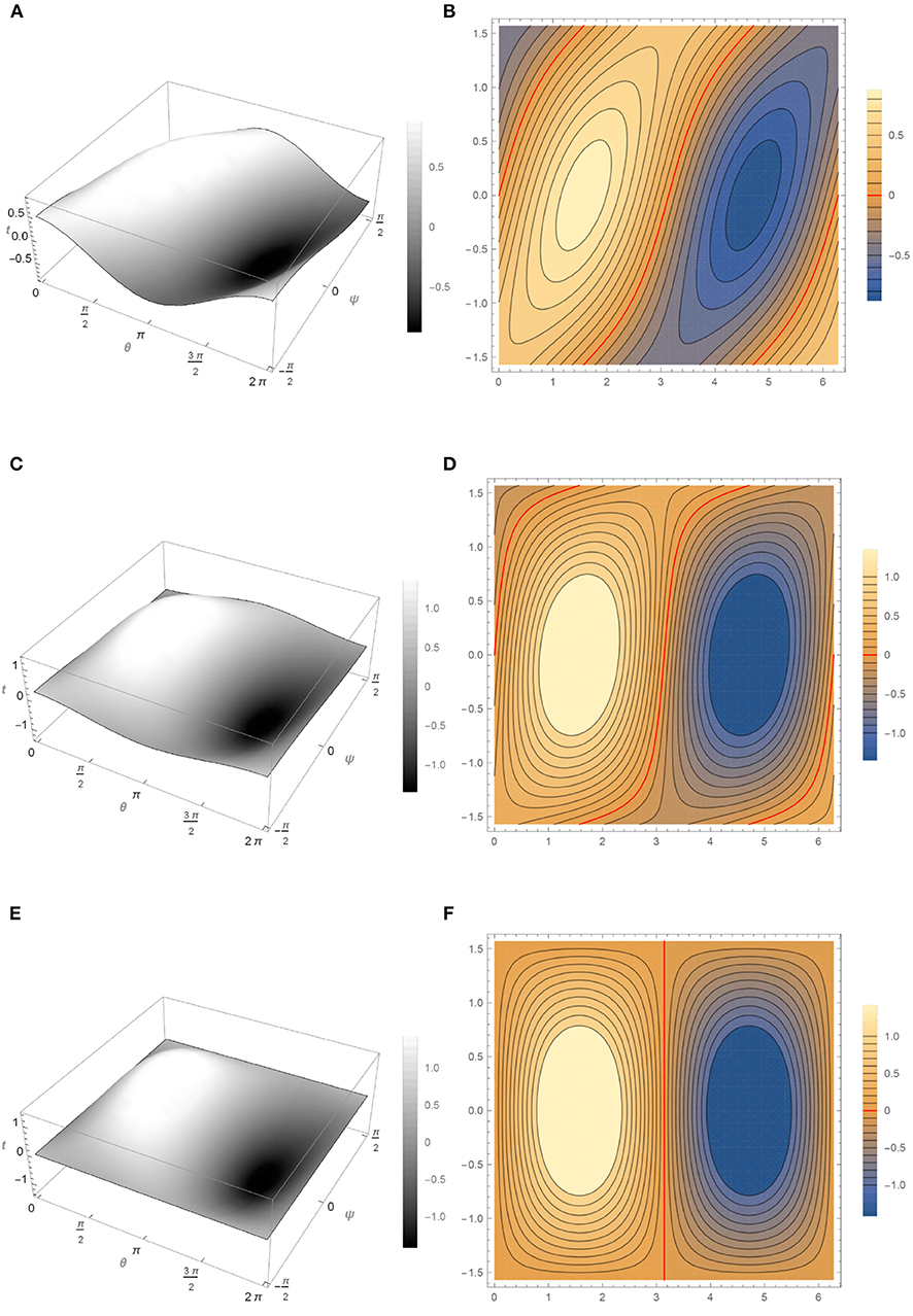
Figure 5. Behavior of u2(t) for different values of t according to Equations (34)–(36). (A) Graph of u2(0). (B) Level curves of u2(0). (C) Graph of u2(0.0055). (D) Level curves of u1(0.0055). (E) Graph of u2(0.02). (F) Level curves of u2(0.02).
All the numerical simulations show that the graph of the solution on S2 approaches values close to 1 and − 1 when t increases, as can be seen in Figures 3A,C,E–5A,C,E found in grayscale color, while in the Figures 3B,D, 4B,D, the transition layer (show in red color) takes place along the level set θ = π which is a closed geodesic (great circle). It can also be noted that in Figure 5B the transition layer at the value t = 0 is not a straight line, but as t increases, this curve becomes a straight line, θ = π, as mentioned above. This suggests that, for ϵ sufficiently small, the attractor will consist of functions concentrating in −1 or +1 with transitions along great circles.
All datasets generated for this study are included in the article/supplementary material.
All authors listed have made a substantial, direct and intellectual contribution to the work, and approved it for publication.
The authors declare that the research was conducted in the absence of any commercial or financial relationships that could be construed as a potential conflict of interest.
1. ^A closed and compact surface enclosing a strictly convex set in ℝ3.
1. Hutchinson JE, Tonewaga Y. Convergence of phase interfaces in the van der Waals - Cahn - Hilliard theory. Calc Var. (2000) 10:49–84. doi: 10.1007/PL00013453
2. Padilla P, Tonewaga Y. On the convergence of stable phase transitions. Commun Pure Appl Math. (1998) 51: 551–79.
3. Bronsard L, Kohn RV. Motion by mean curvature as the singular limit of Ginzburg-Landau dynamics. J Diff Equat. (1991) 90:211–37.
4. Garza-Hume CE, Padilla P. Closed geodesics on oval surfaces and pattern formation. Commun Anal Geometry. (2003) 11, 223–33. doi: 10.4310/CAG.2003.v11.n2.a3
5. Poincaré H. Sur les lignes géodésiques des surfaces convexes. Trans Am Math Soc. (1905) 6:237–74.
6. Berger MS, Bombieri E. On Poincaré's isoperimetric problem for simple closed goedesic. J Funct Anal. (1981) 42:274–98.
7. Temam R. Infinite Dimensional Dynamical Systems in Mechanics and Physics. New York, NY: Springer - Verlag (1999).
9. Robinson JC. Infinite-Dimensional Dynamical Systems An Introduction to Dissipative Parabolic PDEs and the Theory of Global Attractors. New York, NY: Cambridge University Press (2001).
10. Evans LC. Partial Differential Equations, Graduate Studies in Mathematics, Vol. 19. Providence, RI: American Mathematical Society (2000).
11. Hebey E. Nonlinear Analysis on Manifolds: Sobolev Spaces and Inequalities. Providence, RI: American Mathematical Society (2000).
12. Aubin T. Nonlinear Analysis on Manifolds. Monge - Ampère Equations. New York, NY: Springer - Verlag (1982).
14. Del Río H, Garza C, Padilla P. Geodesics, soap bubbles and pattern formation in Riemannian surfaces. J Geometr Anal. (2003) 13:595–604. doi: 10.1007/BF02921880
15. Kythe PK, Puri P, Schferkotter MR. Partial Differential Equations and Boundary Value Problems with Mathematica. 2nd ed. Boca Raton, FL: Chapman and Hall (2003).
Keywords: attractors, parabolic semiflow, closed geodesics, Galerkin method, oval surfaces
Citation: Medina D and Padilla P (2020) The Global Attractor of the Allen-Cahn Equation on the Sphere. Front. Appl. Math. Stat. 6:20. doi: 10.3389/fams.2020.00020
Received: 20 February 2020; Accepted: 07 May 2020;
Published: 17 June 2020.
Edited by:
Jesus Martin-Vaquero, University of Salamanca, SpainReviewed by:
Bulent Karasozen, Middle East Technical University, TurkeyCopyright © 2020 Medina and Padilla. This is an open-access article distributed under the terms of the Creative Commons Attribution License (CC BY). The use, distribution or reproduction in other forums is permitted, provided the original author(s) and the copyright owner(s) are credited and that the original publication in this journal is cited, in accordance with accepted academic practice. No use, distribution or reproduction is permitted which does not comply with these terms.
*Correspondence: Pablo Padilla, cGFibG9AbXltLmlpbWFzLnVuYW0ubXg=
Disclaimer: All claims expressed in this article are solely those of the authors and do not necessarily represent those of their affiliated organizations, or those of the publisher, the editors and the reviewers. Any product that may be evaluated in this article or claim that may be made by its manufacturer is not guaranteed or endorsed by the publisher.
Research integrity at Frontiers
Learn more about the work of our research integrity team to safeguard the quality of each article we publish.