Convergence of a Relaxed Variable Splitting Coarse Gradient Descent Method for Learning Sparse Weight Binarized Activation Neural Network

Sparsification of neural networks is one of the effective complexity reduction methods to improve efficiency and generalizability. Binarized activation offers an additional computational saving for inference. Due to vanishing gradient issue in training networks with binarized activation, coarse gradient (a.k.a. straight through estimator) is adopted in practice. In this paper, we study the problem of coarse gradient descent (CGD) learning of a one hidden layer convolutional neural network (CNN) with binarized activation function and sparse weights. It is known that when the input data is Gaussian distributed, no-overlap one hidden layer CNN with ReLU activation and general weight can be learned by GD in polynomial time at high probability in regression problems with ground truth. We propose a relaxed variable splitting method integrating thresholding and coarse gradient descent. The sparsity in network weight is realized through thresholding during the CGD training process. We prove that under thresholding of ℓ₁, ℓ₀, and transformed-ℓ₁ penalties, no-overlap binary activation CNN can be learned with high probability, and the iterative weights converge to a global limit which is a transformation of the true weight under a novel sparsifying operation. We found explicit error estimates of sparse weights from the true weights.

1. Introduction

Deep neural networks (DNN) have achieved state-of-the-art performance on many machine learning tasks such as speech recognition [1], computer vision [2], and natural language processing [3]. Training such networks is a problem of minimizing a high-dimensional non-convex and non-smooth objective function, and is often solved by first-order methods such as stochastic gradient descent (SGD). Nevertheless, the success of neural network training remains to be understood from a theoretical perspective. Progress has been made in simplified model problems. Blum and Rivest [4] showed that even training a three-node neural network is NP-hard, and Shamir [5] showed learning a simple one-layer fully connected neural network is hard for some specific input distributions. Recently, several works [6, 7] focused on the geometric properties of loss functions, which is made possible by assuming that the input data distribution is Gaussian. They showed that SGD with random or zero initialization is able to train a no-overlap neural network in polynomial time.

Another prominent issue is that DNNs contain millions of parameters and lots of redundancies, potentially causing over-fitting and poor generalization [8] besides spending unnecessary computational resources. One way to reduce complexity is to sparsify the network weights using an empirical technique called pruning [9] so that the non-essential ones are zeroed out with minimal loss of performance [10–12]. Recently a surrogate ℓ₀ regularization approach based on a continuous relaxation of Bernoulli random variables in the distribution sense is introduced with encouraging results on small size image data sets [13]. This motivated our work here to study deterministic regularization of ℓ₀ via its Moreau envelope and related ℓ₁ penalties in a one hidden layer convolutional neural network model [7]. Moreover, we consider binarized activation which further reduces computational costs [14].

The architecture of the network is illustrated in Figure 1 similar to Brutzkus and Globerson [7]. We consider the convolutional setting in which a sparse filter w ∈ ℝ^d is shared among different hidden nodes. The input sample is Z ∈ ℝ^k×d. Note that this is identical to the one layer non-overlapping case where the input is x ∈ ℝ^k×d with k non-overlapping patches, each of size d. We also assume that the vectors of Z are i.i.d. Gaussian random vectors with zero mean and unit variance. Let ${G}$ denote this distribution. Finally, let σ denote the binarized ReLU activation function, σ(z): = χ_{z>0} which equals 1 if z > 0, and 0 otherwise. The output of the network in Figure 1 is given by:

$\begin{array}{ll}h(w,Z)=1^T\sigma (Zw).& (1)\end{array}$

We address the realizable case, where the response training data is mapped from the input training data Z by Equation (1) with a ground truth unit weight vector w^*. The input training data is generated by sampling m training points Z¹, .., Z^m from a Gaussian distribution. The learning problem seeks w to minimize the empirical risk function:

$\begin{array}{ll}l(w,Z):=\frac{1}{m}{\displaystyle \sum _{j=1}^m}{(h(w,Z^j)-h(w^{*},Z^j))}^2& (2)\end{array}$

Due to binarized activation, the gradient of l in w is almost everywhere zero, hence in-effective for descent. Instead, an approximate gradient on the coarse scale, the so called coarse gradient (denoted as ${\tilde{\nabla }}_{w}l$) is adopted as proxy and is proved to drive the iterations to global minimum [14].

FIGURE 1

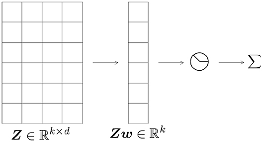
Figure 1. The architecture of a no-overlap neural network.

In the limit m ↑ ∞, the empirical risk l converges to the population risk:

$\begin{array}{ll}f(w):={𝔼}_{Z~G}\left[{(h(w,Z)-h(w^{*},Z))}^2\right]& (3)\end{array}$

which is more regular in w than l. However, the “true gradient” ∇_wf is inaccessible in practice. On the other hand, the coarse gradient ${\tilde{\nabla }}_{w}l$ in the limit m ↑ ∞ forms an acute angle with the true gradient [14]. Hence the expected coarse gradient descent (CGD) essentially minimizes the population risk f as desired.

Our task is to sparsify w in CGD. We note that the iterative thresholding algorithms (IT) are commonly used for retrieving sparse signals [[15–19] and references therein]. In high dimensional setting, IT algorithms provide simplicity and low computational cost, while also promote sparsity of the target vector. We shall investigate the convergence of CGD with simultaneous thresholding for the following objective function

$\begin{array}{ll}\varphi (w)=f(w)+\lambda P(w)& (4)\end{array}$

where f(w) is the population loss function of the network, and P is ℓ₀, ℓ₁, or the transformed-ℓ₁ (Tℓ₁) function: a one parameter family of bilinear transformations composed with the absolute value function [20, 21]. When acting on vectors, the Tℓ₁ penalty interpolates ℓ₀ and ℓ₁ with thresholding in closed analytical form for any parameter value [19]. The ℓ₁ thresholding function is known as soft-thresholding [15, 22], and that of ℓ₀ the hard-thresholding [17, 18]. The thresholding part should be properly integrated with CGD to be applicable for learning CNNs. As pointed out in Louizos et al. [13], it is beneficial to attain sparsity during the optimization (training) process.

1.1. Contribution

We propose a Relaxed Variable Splitting (RVS) approach combining thresholding and CGD for minimizing the following augmented objective function

$\begin{array}{l}{{L}}_{\beta }(u,w)=f(w)+\lambda P(u)+\frac{\beta }{2}{\Vert w-u\Vert }^2\end{array}$

for a positive parameter β. We note in passing that minimizing ${{L}}_{\beta }$ in u recovers the original objective (4) with penalty P replaced by its Moreau envelope [23]. We shall prove that our algorithm (RVSCGD), alternately minimizing u and w, converges for ℓ₀, ℓ₁, and Tℓ₁ penalties to a global limit $(\bar{w},\bar{u})$ with high probability. A key estimate is the Lipschitz inequality of the expected coarse gradient (Lemma 4). Then the descent of Lagrangian function (9) and the angles between the iterated w and w^* follows. The $\bar{w}$ is a novel shrinkage of the true weight w^* up to a scalar multiple. The $\bar{u}$ is a sparse approximation of w^*. To our best knowledge, this result is the first to establish the convergence of CGD for sparse weight binarized activation networks. In numerical experiments, we observed that the $\bar{u}$ limit of RVSCGD with the ℓ₀ penalty recovers sparse w^* accurately.

1.2. Outline

In section 2, we briefly overview related mathematical results in the study of neural networks and complexity reduction. Preliminaries are in section 3. In section 4, we state and discuss the main results. The proofs of the main results are in section 5, and conclusion in section 6.

2. Related Work

In recent years, significant progress has been made in the study of convergence in neural network training. From a theoretical point of view, optimizing (training) neural network is a non-convex non-smooth optimization problem. Blum and Rivest [4], Livni et al. [24], Shalev-Shwartz et al. and [25] showed that training a neural network is hard in the worst cases. Shamir [5] showed that if either the target function or input distribution is “nice,” optimization algorithms used in practice can succeed. Optimization methods in deep neural networks are often categorized into (stochastic) gradient descent methods and others.

Stochastic gradient descent methods were first proposed by Robbins and Monro [26]. The popular back-propagation algorithm was introduced in Rumelhart et al. [27]. Since then, many well-known SGD methods with adaptive learning rates were proposed and applied in practice, such as the Polyak momentum [28], AdaGrad [29], RMSProp [30], Adam [31], and AMSGrad [32].

The behavior of gradient descent methods in neural networks is better understood when the input has Gaussian distribution. Tian [6] showed that the population gradient descent can recover the true weight vector with random initialization for one-layer one-neuron model. Brutzkus and Globerson [7] proved that a convolution filter with non-overlapping input can be learned in polynomial time. Du et al. [33] showed (stochastic) gradient descent with random initialization can learn the convolutional filter in polynomial time and the convergence rate depends on the smoothness of the input distribution and the closeness of patches. Du et al. [34] analyzed the polynomial convergence guarantee of randomly initialized gradient descent algorithm for learning a one-hidden-layer convolutional neural network. A hybrid projected SGD (so called BinaryConnect) is widely used for training various weight quantized DNNs [35, 36]. Recently, a Moreau envelope based relaxation method (BinaryRelax) is proposed and analyzed to advance weight quantization in DNN training [37]. Also a blended coarse gradient descent method [14] is introduced to train fully quantized DNNs in weights and activation functions, and overcome vanishing gradients. For earlier work on coarse gradient (a.k.a. straight through estimator) (see [38–40] among others).

Non-SGD methods for deep learning include the Alternating Direction Method of Multipliers (ADMM) to transform a fully-connected neural network into an equality-constrained problem [41]; method of auxiliary coordinates (MAC) to replace a nested neural network with a constrained problem without nesting [42]. Zhang et al. [43] handled deep supervised hashing problem by an ADMM algorithm to overcome vanishing gradients.

For a similar model to (9) and treatment in a general context (see [44]); and in image processing (see [45]).

3. Preliminaries

3.1. The One-Layer Non-overlap Network

Consider the network introduced in Figure 1. Let σ denote the binarized ReLU activation function, σ(z): = χ_{z>0}. The training sample loss is

$\begin{array}{ll}l(w,Z):=\frac{1}{2}{(1^T\sigma (Zw)-1^T\sigma (Z{w}^{*}))}^2,& (5)\end{array}$

where w^* ∈ ℝ^d is the underlying (non-zero) teaching parameter. Note that (5) is invariant under scaling w → w/c, w^* → w^*/c, for any scalar c > 0. Without loss of generality, we assume ‖w^*‖ = 1. Given independent training samples {Z¹, …, Z^N}, the associated empirical risk minimization reads

$\begin{array}{ll}{\displaystyle \underset{w\in {ℝ}^d}{min}}\frac{1}{N}{\displaystyle \sum _{i=1}^N}l(w,Z^i).& (6)\end{array}$

The empirical risk function in (6) is piece-wise constant and has i.e., zero partial w gradient. If σ were differentiable, then back-propagation would rely on:

$\begin{array}{ll}\frac{\partial l}{\partial w}(w,Z)=Z^T{\sigma }^{\prime }(Zw)(\sigma (Zw)-\sigma (Z{w}^{*})).& (7)\end{array}$

However, σ has zero derivative i.e., rendering (7) inapplicable. We study the coarse gradient descent with σ′ in (7) replaced by the (sub)derivative μ′ of the regular ReLU function μ(x): = max(x, 0). More precisely, we use the following surrogate of $\frac{\partial l}{\partial w}(w,Z)$:

$\begin{array}{ll}g(w,Z)=\sqrt{\frac{2}{\pi }}{Z}^T{\mu }^{\prime }(Zw)(\sigma (Zw)-\sigma (Z{w}^{*}))& (8)\end{array}$

with μ′(x) = σ(x). The constant $\sqrt{\frac{2}{\pi }}$ represents a ReLU function μ with smaller slope, and will be necessary to give a stronger convergence result for our main findings. To simplify our analysis, we let N ↑ ∞ in (6), so that its coarse gradient approaches 𝔼_Z[g(w, Z)]. The following lemma asserts that 𝔼_Z[g(w, Z)] has positive correlation with the true gradient ∇f(w), and consequently, −𝔼_Z[g(w, Z)] gives a reasonable descent direction.

Lemma 1. [14] If θ(w, w^*) ∈ (0, π), and ‖w‖ ≠ 0, then the inner product between the expected coarse and true gradient w.r.t. w is

$\langle {𝔼}_Z[g(w,Z)],\nabla f(w)\rangle =\frac{sin(\theta (w,w^{*}))}{4{\pi }^2\Vert w\Vert }{k}^2\ge 0.$

3.2. The Relaxed Variable Splitting Coarse Gradient Descent Method

Suppose we want to train the network in a way that w^t converges to a limit $\bar{w}$ in some neighborhood of w^*, and we also want to promote sparsity in the limit $\bar{w}$. A classical approach is to minimize the Lagrangian: ϕ(w) = f(w) + λ‖w‖₁, for some λ > 0. In practice, the ℓ₁ penalty can also be replaced by ℓ₀ or Tℓ₁. Our proposed relaxed variable splitting (RVS) proceeds by first extending ϕ into a function of two variables f(w) + λ‖u‖₁, and consider the augmented Lagrangian:

$\begin{array}{ll}{{L}}_{\beta }(u,w)=f(w)+\lambda {\Vert u\Vert }_1+\frac{\beta }{2}{\Vert w-u\Vert }^2& (9)\end{array}$

Let S_α be the soft thresholding operator, S_α(x) = sgn(x) max{|x| − α, 0}. The resulting RSVCGD method is described in Algorithm 1:

ALGORITHM 1

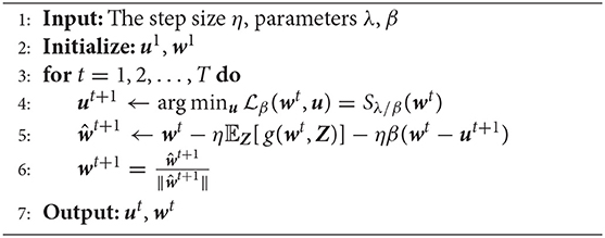
Algorithm 1: RVSCGD Algorithm

3.3. Comparison With ADMM

A well-known, modern method to solve the minimization problem ϕ(w) = f(w) + λ‖w‖₁ is the Alternating Direction Method of Multipliers (or ADMM). In ADMM, we consider the Lagrangian

$\begin{array}{ll}{{L}}_{\beta }(w,u,z)=f(w)+\lambda {\Vert u\Vert }_1+\langle z,w-u\rangle +\frac{\beta }{2}{\Vert w-u\Vert }^2.& (10)\end{array}$

and apply the updates:

$\begin{array}{ll}\{\begin{array}{l}{w}^{t+1}\leftarrow arg{\displaystyle {min}_w}{{L}}_{\beta }(w,u^t,z^t)\\ u^{t+1}\leftarrow arg{\displaystyle {min}_u}{{L}}_{\beta }(w^{t+1},u,z^t)\\ z^{t+1}\leftarrow z^t+\beta (w^{t+1}-u^{t+1})\end{array}& (11)\end{array}$

Although widely used in practice, the ADMM method has several drawbacks when it comes to regularizing deep neural networks: Firstly, the ℓ₁ penalty is often replaced by ℓ₀ in practice; but ‖·‖₀ is non-differentiable and non-convex, thus current theory in optimization does not apply [46]. Secondly, the update $w^{t+1}\leftarrow arg\underset{w}{min}{{L}}_{\beta }(w^{t+1},u,z^t)$ is not applicable in practice on DNN, as it requires one to know fully how f(w) behaves. In most ADMM adaptations on DNN, this step is replaced by a simple gradient descent. Lastly, the Lagrange multiplier z^t tends to reduce the sparsity of the limit of u^t, as it seeks to close the gap between w^t and u^t.

In contrast, the RVSCGD method resolves all these difficulties presented by ADMM. Firstly, without the linear term 〈z, w − u〉, one has an explicit formula for the update of u, which can be easily implemented. Secondly, the update of w^t is not an argmin update, but rather a gradient descent iteration itself, so our theory does not deviate from practice. Lastly, without the Lagrange multiplier term z^t, there will be a gap between w^t and u^t at the limit. The u^t is much more sparse than in the case of ADMM, and numerical results showed that f(w^t) and f(u^t) behave very similarly on deep networks. An intuitive explanation for this is that when the dimension of w^t is high, most of its components that will be pruned off to get u^t have very small magnitudes, and are often the redundant weights.

In short, the RVSCGD method is easier to implement (no need to keep track of the variable z^t), can greatly increase sparsity in the weight variable u^t, while also maintaining the same performance as the ADMM method. Moreover, RVSCGD has convergence guarantee and limit characterization as stated below.

4. Main Results

Theorem 1. Suppose that the initialization and penalty parameters of the RVSCGD algorithm satisfy:

(i) θ(w⁰, w^*) ≤ π − δ, for some δ > 0;

(ii) $\beta \le \frac{ksin\delta }{2\sqrt{2\pi }}$, and $\lambda <\frac{k}{2\sqrt{2\pi d}}$;

(iii) η is small such $\eta \le min\left\{\frac{1}{\beta +L},\frac{2\sqrt{2\pi }}{k}\right\}$, where L is the Lipschitz constant in Lemma 4; and for all t, $\eta \Vert {𝔼}_Z[g(w^t,Z)]+\beta (w^t-u^{t+1})\Vert \le \frac{1}{2}$.

Then the Lagrangian ${{L}}_{\beta }(u^t,w^t)$ decreases monotonically; and (u^t, w^t) converges sub-sequentially to a limit point $(\bar{u},\bar{w})$, with $\bar{u}=S_{\lambda /\beta }(\bar{w})$, such that:

(i) Let $\theta :=\theta (\bar{w},w^{*})$ and $\gamma :=\theta (\bar{u},\bar{w})$, then θ < δ;

(ii) The limit point $(\bar{u},\bar{w})$ satisfies $\bar{u}=S_{\lambda /\beta }(\bar{w})$ and

$\begin{array}{ll}{w}^{*}=\frac{2\sqrt{2\pi }}{k}\beta (\bar{w}-S_{\lambda /\beta }(\bar{w}))+C\bar{w}& (12)\end{array}$

where S_λ/β(·) is the soft-thresholding operator of ℓ₁, for some constant $C\ge \frac{k-2\lambda \sqrt{2\pi d}}{k}$;

(iii) The limit point $\bar{w}$ is close to the ground truth w^* such that

$\begin{array}{ll}\Vert w^{*}-\bar{w}\Vert \le \frac{4\sqrt{2\pi }\beta sin\gamma }{k}.& (13)\end{array}$

Remark 1. As the sign of $(\bar{w}-S_{\lambda /\beta }(\bar{w}))$ agrees with $\bar{w}$, Equation (12) implies that w^* equals an expansion of $C\bar{w}$ or equivalently $\bar{w}$ is (up to a scalar multiple) a shrinkage of w^*, which explains the source of sparsity in $\bar{\text{w}}$. The assumption on η is reasonable, as will be shown below: $\Vert {𝔼}_Z[g(w^t,Z)]\Vert$ is bounded away from zero, and thus $\Vert {𝔼}_Z[g(w^t,Z)]+\beta (w^t-u^{t+1})\Vert$ is also bounded.

The proof is provided in details in section 5. Here we provide an overview of the key steps. First, we show that there exists a constant L_f such that

$\Vert \nabla f(w^{t+1})-\nabla f(w^t)\Vert \le L_f\Vert w^{t+1}-w^t\Vert$

then we show that the Lipschitz gradient property still holds when replaced by the coarse gradient:

$\Vert {𝔼}_Z[g(w^{t+1},Z)]-{𝔼}_Z[g(w^t,Z)]\Vert \le K\Vert w^{t+1}-w^t\Vert$

and subsequently show

$\begin{array}{l}f(w_2)-f(w_1)\le \langle {𝔼}_Z[g(w_1,Z)],w_2-w_1\rangle +\frac{L}{2}{\Vert w_2-w_1\Vert }^2.\end{array}$

These inequalities hold when ‖w^t‖ ≥ M, for some M > 0. It can be shown that with bad initialization, one may have ‖w^t‖ → 0 as t → ∞. We circumvent this problem by normalizing w^t at each iteration.

Next, we show the iterations satisfy θ^t+1 ≤ θ^t, and ${{L}}_{\beta }(u^{t+1},w^{t+1})\le {{L}}_{\beta }(u^t,w^t)$. Finally, an analysis of the stationary point yields the desired bound.

In none of these steps do we use convexity of the ℓ₁ penalty term. Here we extend our result to ℓ₀ and transformed ℓ₁ (Tℓ₁) regularization [21].

Corollary 1.1. Suppose that the initialization of the RVSCGD algorithm satisfies the conditions in Theorem 1, and that the ℓ₁ penalty is replaced by ℓ₀ or Tℓ₁. Then the RVSCGD iterations converge to a limit point $(\bar{u},\bar{w})$ satisfying Equation (12) with ℓ₀'s hard thresholding operator [18] or Tℓ₁ thresholding [19] replacing S_λ/β, and similar bound (13) holds.

5. Proof of Main Results

The following Lemmas give an outline for the proof of Theorem 1.

Lemma 2. If every entry of Z is i.i.d. sampled from ${N}(0,1),\Vert w^{*}\Vert =1$, and ‖w‖ ≠ 0, then the true gradient of the population loss f(w) is

$\begin{array}{ll}\nabla f(w)=\frac{-k}{2\pi \Vert w\Vert }\frac{\left(\text{I}-\frac{w{w}^T}{{\Vert w\Vert }^2}\right)w^{*}}{\Vert \left(\text{I}-\frac{w{w}^T}{{\Vert w\Vert }^2}\right)w^{*}\Vert },& (14)\end{array}$

for θ(w, w^*) ∈ (0, π); and the expected coarse gradient w.r.t. w is

$\begin{array}{ll}{𝔼}_Z[g(w,Z)]=\frac{k}{\pi }\left[\frac{w}{\Vert w\Vert }-cos\left(\frac{\theta (w,w^{*})}{2}\right)\frac{\frac{w}{\Vert w\Vert }+w^{*}}{\Vert \frac{w}{\Vert w\Vert }+w^{*}\Vert }\right]& (15)\end{array}$

Lemma 3. (Properties of true gradient)

Given w₁, w₂ with min{‖w₁‖, ‖w₂‖} = c > 0 and max{‖w₁‖, ‖w₂‖} = C, there exists a constant L_f > 0 depends on c and C such that

$\begin{array}{l}\Vert \nabla f(w_1)-\nabla f(w_2)\Vert \le L_f\Vert w_1-w_2\Vert \end{array}$

Moreover, we have

$\begin{array}{l}f(w_2)\le f(w_1)+\langle \nabla f(w_1),w_2-w_1\rangle +\frac{L_f}{2}{\Vert w_2-w_1\Vert }^2.\end{array}$

Lemma 4. (Properties of expected coarse gradient)

If w₁, w₂ satisfy $\frac{1}{2}\le \Vert w_1\Vert ,\Vert w_2\Vert \le \frac{3}{2}$, and $\theta (w_1,w^{*}),\theta (w_2,w^{*})\in (0,\pi )$, then there exists a constant K such that

$\begin{array}{ll}\Vert {𝔼}_Z[g(w_1,Z)]-{𝔼}_Z[g(w_2,Z)]\Vert \le K\Vert w_1-w_2\Vert & (16)\end{array}$

Moreover, there exists a constant L such that

$\begin{array}{ll}f(w_2)-f(w_1)\le \langle {𝔼}_Z[g(w_1,Z)],w_2-w_1\rangle +\frac{L}{2}{\Vert w_2-w_1\Vert }^2.& (17)\end{array}$

Remark 2. The condition $\frac{1}{2}\le \Vert w_1\Vert ,\Vert w_2\Vert \le \frac{3}{2}$ in Lemma 4 is to match the RVSCGD algorithm and to give an explicit value for K. The result still holds in general when 0 < c ≤ ‖w₁‖, ‖w₂‖ ≤ C. Compared to Lemma 3, when $c=\frac{1}{2}$ and $C=\frac{1}{2}$, one has $L_f=\frac{4\sqrt{k}}{\pi }$, which is a sharper bound than $K=\frac{k}{\sqrt{2\pi }}$ in the coarse gradient case.

Lemma 5. (Angle Descent)

Let θ^t: = θ(w^t, w^*). Suppose the initialization of the RVSCGD algorithm satisfies θ⁰ ≤ π − δ and $\beta \le \frac{ksin\delta }{2\sqrt{2\pi }}$, then θ^t+1 ≤ θ^t.

Lemma 6. (Lagrangian Descent)

Suppose the initialization of the RVSCGD algorithm satisfies $\eta \le \frac{1}{\beta +L}$, where L is the Lipschitz constant in Lemma 4, then ${{L}}_{\beta }(u^{t+1},w^{t+1})\le {{L}}_{\beta }(u^t,w^t)$.

Lemma 7. (Properties of limit point)

Suppose the initialization of the RVSCGD algorithm satisfies: θ(w⁰, w^*) ≤ π − δ, for some δ > 0, λ is small such that $\frac{2\sqrt{2\pi }}{k}\lambda \sqrt{d}<1$, and η is small such that $\eta \frac{k}{2\sqrt{2\pi }}<1$. Let $\theta :=\theta (\bar{w},w^{*})$ and $\gamma :=\theta (\bar{u},\bar{w})$, then (u^t, w^t) converges to a limit point $(\bar{u},\bar{w})$ such that

$\theta <\delta \text{ and }\Vert w^{*}-\bar{w}\Vert \le \frac{4\sqrt{2\pi }\beta sin\gamma }{k}.$

Lemmas 2, 3 follow directly from Yin et al. [14]. The proof of Lemmas 4, 5, 6, 7 are provided below.

5.1. Proof of Lemma 4

First suppose ‖w₁‖ = ‖w₂‖ = 1. By Lemma 2, we have

$\begin{array}{l}{𝔼}_Z[g(w_j,Z)]=\frac{k}{\pi }\left[w_j-cos\left(\frac{\theta (w_j,w^{*})}{2}\right)\frac{w_j+w^{*}}{\Vert w_j+w^{*}\Vert }\right]\end{array}$

for j = 1, 2. Consider the plane formed by w_j and w^*, since ‖w^*‖ = 1, we have an equilateral triangle formed by w_j and w^* (see Figure 2).

FIGURE 2

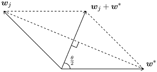
Figure 2. Geometry of w^t and w^* when ‖w^t‖ = ‖w^*‖ = 1.

Simple geometry shows

$cos\left(\frac{\theta (w_j,w^{*})}{2}\right)=\frac{\frac{1}{2}\Vert w_j+w^{*}\Vert }{\Vert w^{*}\Vert }=\frac{1}{2}\Vert w_j+w^{*}\Vert$

Thus the expected coarse gradient simplifies to

$\begin{array}{ll}{𝔼}_Z[g(w_j,Z)]=\frac{k}{\pi }\left[w_j-\frac{w_j+w^{*}}{2}\right]=\frac{k}{2\pi }{w}_j-\frac{k}{2\pi }{w}^{*}& (18)\end{array}$

which implies

$\begin{array}{ll}\Vert {𝔼}_Z\left[g(w_1,Z)\right]-{𝔼}_Z\left[g(w_2,Z)\right]\Vert \le K\Vert w_1-w_2\Vert & (19)\end{array}$

with $K=\frac{k}{2\pi }$.

Now suppose $\frac{1}{2}\le \Vert w_1\Vert ,\Vert w_2\Vert \le \frac{3}{2}$. By Equation (15), we have ${𝔼}_Z[g(w,Z)]={𝔼}_Z[g(\frac{w}{C},Z)]$, for all C > 0. Then,

$\begin{array}{l}\Vert {𝔼}_Z[g(w_1,Z)]-{𝔼}_Z[g(w_2,Z)]\Vert \\ =\Vert {𝔼}_Z\left[g\left(\frac{w_1}{\Vert w_1\Vert },Z\right)\right]-{𝔼}_Z\left[g\left(\frac{w_2}{\Vert w_2\Vert },Z\right)\right]\Vert \\ \le K^{\prime }\Vert \frac{w_1}{\Vert w_1\Vert }-\frac{w_2}{\Vert w_2\Vert }\Vert \\ \le 2K^{\prime }\Vert w_1-w_2\Vert \end{array}$

where the first inequality follows from (19), and the second inequality is from the constraint $\frac{1}{2}\le \Vert w_1\Vert ,\Vert w_2\Vert \le \frac{3}{2}$, with equality when $\Vert w_1\Vert =\Vert w_2\Vert =\frac{1}{2}$. Letting $K=2K^{\prime }=\frac{k}{\pi }$, the first claim is proved.

It remains to show the gradient descent inequality. By Yin et al. [14], we have

$\begin{array}{l}f(w)=\frac{1}{8}[1^T(I+11^T)1-21^T\left(\left(1-\frac{2}{\pi }\theta (w,w^{*})\right)I+11^T\right)1\hfill \\ +1^T(I+11^T)1]\hfill \end{array}$

Let ${\theta }_1=\theta (w_1,w^{*}),{\theta }_2=\theta (w_2,w^{*})$. Then

$\begin{array}{l}f(w_2)-f(w_1)=\frac{1}{4}\left[1^T\left(\left(\frac{2}{\pi }{\theta }_2-\frac{2}{\pi }{\theta }_1\right)I\right)1\right]=\frac{k}{2\pi }({\theta }_2-{\theta }_1)\end{array}$

We will show

$\begin{array}{l}f(w_2)-f(w_1)\le \langle {𝔼}_Z[g(w_1,Z)],w_2-w_1\rangle +L{\Vert w_2-w_1\Vert }^2\end{array}$

for ‖w₁‖ = ‖w₂‖ = 1 and θ₂ ≤ θ₁. By Equation (18),

${𝔼}_Z[g(w_1,Z)]=\frac{k}{2\pi }(w_1-w^{*})$

It remains to show

$\begin{array}{l}\frac{k}{2\pi }({\theta }_2-{\theta }_1)\le \langle \frac{k}{2\pi }(w_1-w^{*}),w_2-w_1\rangle +L{\Vert w_2-w_1\Vert }^2\end{array}$

or there exists a constant K₁ such that

${\theta }_2-{\theta }_1\le \langle w_1-w^{*},w_2-w_1\rangle +K_1{\Vert w_2-w_1\Vert }^2$

Notice that by writing $K_1=\frac{1}{2}+K_2$, we have

$\begin{array}{l}\langle w_1-w^{*},w_2-w_1\rangle +K_1{\Vert w_2-w_1\Vert }^2\\ =\langle w_1-w^{*},w_2-w_1\rangle +K_1\langle w_2-w_1,w_2-w_1\rangle \\ =\langle w_1-w^{*},w_2-w_1\rangle +\frac{1}{2}\langle w_2-w_1,w_2-w_1\rangle +K_2{\Vert w_2-w_1\Vert }^2\\ =\langle \frac{1}{2}{w}_1+\frac{1}{2}{w}_2-w^{*},w_2-w_1\rangle +K_2{\Vert w_2-w_1\Vert }^2\\ =\langle -w^{*},w_2-w_1\rangle +\frac{1}{2}\langle w_1+w_2,w_2-w_1\rangle +K_2{\Vert w_2-w_1\Vert }^2\\ =\langle -w^{*},w_2-w_1\rangle +K_2{\Vert w_2-w_1\Vert }^2\end{array}$

where the last equality follows since ‖w₁‖ = ‖w₂‖ = 1 implies 〈w₁ + w₂, w₂ − w₁ 〉 = 0. On the other hand,

$\begin{array}{l}\langle -w^{*},w_2-w_1\rangle \\ =-\Vert w^{*}\Vert \Vert w_2\Vert cos{\theta }_2+\Vert w^{*}\Vert \Vert w_1\Vert cos{\theta }_1=cos{\theta }_1-cos{\theta }_2\end{array}$

so it suffices to show there exists a constant K₂ such that

${\theta }_2+cos{\theta }_2-{\theta }_1-cos{\theta }_1\le K_2{\Vert w_2-w_1\Vert }^2$

Notice the function θ ↦ θ + cosθ is monotonically increasing on [0, π]. For θ₁, θ₂ ∈ [0, π] with θ₂ ≤ θ₁, the LHS is non-positive, and the inequality holds. Thus, one can take $K_2=0,K_1=\frac{1}{2}$, and $L=\frac{k}{4\pi }$.

5.2. Proof of Lemma 5

Due to normalization in the RVSCGD algorithm, ‖w^t‖ = 1 for all t. By Equation (18), we have

$\begin{array}{l}{w}^t-\eta {𝔼}_Z[g(w^t,Z)]=\left(1-\eta \frac{k}{2\sqrt{2\pi }}\right)w^t+\eta \frac{k}{2\sqrt{2\pi }}{w}^{*}\end{array}$

and the update of u is the well-known soft-thresholding of w [15, 22]:

$\begin{array}{l}{u}^{t+1}=arg{\displaystyle \underset{u}{min}}{{L}}_{\beta }(u,w^t)=S_{\lambda /\beta }(w^t)\end{array}$

where S_λ/β(·) is the soft-thresholding operator:

$\begin{array}{l}{S}_{\lambda /\beta }(x)=\{\begin{array}{ll}x-\lambda /\beta ,& x>\lambda /\beta \\ 0,& |x|\le \lambda /\beta \\ x+\lambda /\beta ,& x<-\lambda /\beta \end{array}\end{array}$

and S_λ/β(w) applies the thresholding to each component of w. Then the update of w has the form

$\begin{array}{l}{w}^{t+1}=C^t{w}^t+\eta \frac{k}{2\sqrt{2\pi }}{w}^{*}+\eta \beta u^{t+1}\end{array}$

for some constant C^t > 0. Suppose the initialization satisfies θ(w⁰, w^*) ≤ π − δ, for some δ > 0. It suffices to show that if θ^t ≤ π − δ, then θ^t+1 ≤ π − δ. To this end, since $u^{t+1}=S_{\lambda /\beta }(w^t)$, we have $\theta (w^t,u^{t+1})\le \frac{\pi }{2}$. Consider the worst case scenario: w^t, w^*, u^t+1 are co-planar with $\theta (u^{t+1},w^t)=\frac{\pi }{2}$, and w^*, u^t+1 are on two sides of w^t (see Figure 3). We need $\frac{k}{2\sqrt{2\pi }}{w}^{*}+\beta u^{t+1}$ to be in region I. This condition is satisfied when β is small such that

$sin\delta \ge \frac{\beta \Vert u^{t+1}\Vert }{\frac{k}{2\sqrt{2\pi }}\Vert w^{*}\Vert }=\frac{2\sqrt{2\pi }\beta \Vert u^{t+1}\Vert }{k}$

or

$\beta \le \frac{ksin\delta }{2\sqrt{2\pi }\Vert u^{t+1}\Vert }$

since $u^{t+1}=S_{\lambda /\beta }(w^t)$, we have ‖u^t+1‖ ≤ 1. Thus, it suffices to have $\beta \le \frac{ksin\delta }{2\sqrt{2\pi }}$.

FIGURE 3

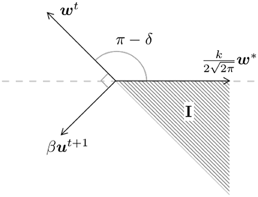
Figure 3. Worst case of the update on w^t.

5.3. Proof of Lemma 6

By definition of the update on u, we have ${{L}}_{\beta }(u^{t+1},w^t)\le {{L}}_{\beta }(u^t,w^t)$. It remains to show ${{L}}_{\beta }(u^{t+1},w^{t+1})\le {{L}}_{\beta }(u^{t+1},w^t)$. First notice that since

$w^{t+1}=C^t(w^t-\eta {𝔼}_Z[g(w^t,Z)]-\eta \beta (w^t-u^{t+1}))$

where C^t > 0 is the normalizing constant, thus

${𝔼}_Z[g(w^t,Z)]=\frac{1}{\eta }\left(w^t-\frac{w^{t+1}}{C^t}\right)-\beta (w^t-u^{t+1})$

For a fixed u: = u^t+1 we have

$\begin{array}{l}{{L}}_{\beta }(u,w^{t+1})-{{L}}_{\beta }(u,w^t)\\ =f(w^{t+1})-f(w^t)+\frac{\beta }{2}({\Vert w^{t+1}-u\Vert }^2-{\Vert w^t-u\Vert }^2)\\ \le \langle {𝔼}_Z[g(w^t,Z)],w^{t+1}-w^t\rangle +\frac{L}{2}{\Vert w^{t+1}-w^t\Vert }^2\\ +\frac{\beta }{2}({\Vert w^{t+1}-u\Vert }^2-{\Vert w^t-u\Vert }^2)\\ =\frac{1}{\eta }\langle w^t-\frac{w^{t+1}}{C^t},w^{t+1}-w^t\rangle -\beta \langle w^t-u,w^{t+1}-w^t\rangle \\ +\frac{L}{2}{\Vert w^{t+1}-w^t\Vert }^2+\frac{\beta }{2}({\Vert w^{t+1}-u\Vert }^2-{\Vert w^t-u\Vert }^2)\\ =\frac{1}{\eta }\langle w^t-\frac{w^{t+1}}{C^t},w^{t+1}-w^t\rangle +\left(\frac{L}{2}+\frac{\beta }{2}\right){\Vert w^{t+1}-w^t\Vert }^2\\ +\frac{\beta }{2}{\Vert w^{t+1}-u\Vert }^2-\frac{\beta }{2}{\Vert w^t-u\Vert }^2-\beta \langle w^t-u,w^{t+1}-w^t\rangle \\ -\frac{\beta }{2}{\Vert w^{t+1}-w^t\Vert }^2\\ =\frac{1}{\eta }\langle w^t-\frac{w^{t+1}}{C^t},w^{t+1}-w^t\rangle +\left(\frac{L}{2}+\frac{\beta }{2}\right){\Vert w^{t+1}-w^t\Vert }^2\end{array}$

Since ‖w^t‖, ‖w^t+1‖ = 1, we know (w^t+1 − w^t) bisects the angle between w^t+1 and −w^t. The assumption $\Vert \eta {𝔼}_Z[g(w^t,Z)]+\eta \beta (w^t-u^{t+1})\Vert \le \frac{1}{2}$ guarantees $\frac{2}{3}\le C^t\le 2$ and θ(−w^t, w^t+1) < π. It follows that θ(w^t+1 − w^t, w^t) and θ(w^t+1 − w^t, w^t+1) are strictly less than $\frac{\pi }{2}$. On the other hand, $\left(\frac{w^{t+1}}{C^t}-w^t\right)$ also lies in the plane bounded by w^t+1 and −w^t. Therefore,

$\theta \left(\frac{w^{t+1}}{C^t}-w^t,w^{t+1}-w^t\right)<\frac{\pi }{2}.$

This implies $\langle \frac{w^{t+1}}{C^t}-w^t,w^{t+1}-w^t\rangle \ge 0$. Moreover, when C^t ≥ 1:

$\begin{array}{l}\langle \frac{w^{t+1}}{C^t}-w^t,w^{t+1}-w^t\rangle =\langle \frac{w^{t+1}}{C^t}-\frac{w^t}{C^t},w^{t+1}-w^t\rangle \\ \hfill -\langle \frac{C^t-1}{C^t}{w}^t,w^{t+1}-w^t\rangle \\ \ge \frac{1}{C^t}{\Vert w^{t+1}-w^t\Vert }^2\end{array}$

And when $\frac{2}{3}\le C^t\le 1$:

$\begin{array}{l}\langle \frac{w^{t+1}}{C^t}-w^t,w^{t+1}-w^t\rangle =\langle w^{t+1}-w^t,w^{t+1}-w^t\rangle \\ \hfill +\langle \frac{1-C^t}{C^t}{w}^{t+1},w^{t+1}-w^t\rangle \\ \ge {\Vert w^{t+1}-w^t\Vert }^2\end{array}$

Thus, we have

$\begin{array}{l}{{L}}_{\beta }(u,w^{t+1})-{{L}}_{\beta }(u,w^t)\le \left(\frac{L}{2}+\frac{\beta }{2}-\frac{{\chi }_{\{C^t\ge 1\}}}{\eta C^t}-\frac{{\chi }_{\{\frac{2}{3}\le C^t\le 1\}}}{\eta }\right)\\ {\Vert w^{t+1}-w^t\Vert }^2\end{array}$

Therefore, if η is small so that $\eta \le \frac{2}{C^t(\beta +L)}$ and $\eta \le \frac{2}{\beta +L}$, the update on w will decrease ${{L}}_{\beta }$. Since C^t ≤ 2, the condition is satisfied when $\eta \le \frac{1}{\beta +L}$.

5.4. Proof of Lemma 7

Since ${{L}}_{\beta }(u^t,w^t)$ is non-negative, by Lemma 5, 6, ${{L}}_{\beta }$ converges to some limit ${L}$. This implies (u^t, w^t) converges to some stationary point $(\bar{u},\bar{w})$. By the update of w^t, we have

$\begin{array}{ll}\bar{w}=\bar{C}(c_1\bar{w}+\eta c_2{w}^{*}+\eta \beta \bar{u})& (20)\end{array}$

for some constant $\bar{C},c_1,c_2>0$, where $c_2=\frac{k}{2\sqrt{2\pi }}$, c₁ > 0 due to our assumption, and $\bar{u}=S_{\lambda /\beta }(\bar{w})$. For expression (20) to hold, we need

$\begin{array}{ll}{c}_2{w}^{*}+\beta \bar{u}//\bar{w}& (21)\end{array}$

Expression (21) implies $\bar{w},\bar{u}$, and w^* are co-planar. Let $\gamma :=\theta (\bar{u},\bar{w})$. From expression (21), and the fact that $\Vert \bar{w}\Vert =\Vert w^{*}\Vert =1$, we have

$\begin{array}{l}{(\langle c_2{w}^{*}+\beta \bar{u},\bar{w}\rangle )}^2={\Vert c_2{w}^{*}+\beta \bar{u}\Vert }^2{\Vert \bar{w}\Vert }^2\end{array}$

which implies $c_2^2{cos}^2\theta +2c_2\beta \Vert \bar{u}\Vert cos\theta cos\gamma +{\beta }^2{\Vert \bar{u}\Vert }^2{cos}^2\gamma =c_2^2+2c_2\beta \Vert \bar{u}\Vert cos(\theta +\gamma )+{\beta }^2{\Vert \bar{u}\Vert }^2$ Recall cos(a+b) = cos a cos b − sin a sin b. Thus,

$\begin{array}{ll}{c}_2^2{sin}^2\theta -2c_2\beta \Vert \bar{u}\Vert sin\theta sin\gamma +{\beta }^2{\Vert \bar{u}\Vert }^2{sin}^2\gamma & =0\end{array}$

which implies

$\begin{array}{ll}\frac{k}{2\sqrt{2\pi }}sin\theta =\beta \Vert \bar{u}\Vert sin\gamma & (22)\end{array}$

By the initialization of β, we have $\frac{k}{2\sqrt{2\pi }}sin\theta <\frac{k}{2\sqrt{2\pi }}sin\delta$. This implies θ < δ.

Finally, expression (20) can also be written as

$\begin{array}{ll}\left(w^{*}-\frac{2\sqrt{2\pi }}{k}\beta (\bar{w}-\bar{u})\right)//\bar{w}& (23)\end{array}$

From expression (23), we see that w^*, after subtracting some vector whose signs agree with $\bar{w}$, and whose non-zero components are at most $\frac{2\sqrt{2\pi }}{k}\lambda$, is parallel to $\bar{w}$. This implies $\bar{w}$ is some soft-thresholded version of w^*, modulo normalization. Moreover, since $\Vert \frac{2\sqrt{2\pi }}{k}\beta (\bar{w}-\bar{u})\Vert \le \frac{2\sqrt{2\pi }}{k}\lambda \sqrt{d}$, for small λ such that $\frac{2\sqrt{2\pi }}{k}\lambda \sqrt{d}<1$, we must have

$\theta \left(w^{*}-\frac{2\sqrt{2\pi }}{k}\beta (\bar{w}-\bar{u}),\bar{w}\right)=0$

On the other hand,

$\begin{array}{l}\Vert w^{*}-\frac{2\sqrt{2\pi }}{k}\beta (\bar{w}-\bar{u})\Vert \ge \Vert w^{*}\Vert -\Vert \frac{2\sqrt{2\pi }}{k}\beta (\bar{w}-\bar{u})\Vert \\ \ge 1-\frac{2\sqrt{2\pi }}{k}\lambda \sqrt{d}\end{array}$

therefore, $w^{*}-\frac{2\sqrt{2\pi }}{k}\beta (\bar{w}-\bar{u})=C\bar{w}$, for some constant C such that $C\ge \frac{k-2\lambda \sqrt{2\pi d}}{k}$.

Finally, consider the equilateral triangle with sides $w^{*},\bar{w}$, and $w^{*}-\bar{w}$. By the law of sines,

$\frac{\Vert w^{*}-\bar{w}\Vert }{sin\theta }=\frac{\Vert w^{*}\Vert }{sin\theta (\bar{w},w^{*}-\bar{w})}=\frac{1}{sin\theta (\bar{w},w^{*}-\bar{w})}$

as θ is small, $\theta (\bar{w},w^{*}-\bar{w})$ is near $\frac{\pi }{2}$. We can assume $sin\theta (\bar{w},w^{*}-\bar{w})\ge \frac{1}{2}$. Together with expression (22), we have

$\Vert w^{*}-\bar{w}\Vert \le 2sin\theta =\frac{4\sqrt{2\pi }\beta \Vert \bar{u}\Vert sin\gamma }{k}\le \frac{4\sqrt{2\pi }\beta sin\gamma }{k}.$

5.5. Proof of Theorem 1

Combining Lemmas 2–7, Theorem 1 is proved.

5.6. Proof of Corollary

Lemma 8. [19] Let

$f_{\lambda ,x}(y)=\frac{1}{2}{(y-x)}^2+\lambda {\rho }_a(y),$

$g_{\lambda }(x)=sgn(x)\left\{\frac{2}{3}(a+|x|)cos\left(\frac{\varphi (x)}{3}\right)-\frac{2a}{3}+\frac{|x|}{3}\right\}$

where $\varphi (x)=arccos\left(1-\frac{27\lambda a(a+1)}{2{(a+|x|)}^3}\right)$. Then $y_{\lambda }^{*}(x)=arg\underset{y}{min}{f}_{\lambda ,x}(y)$ is the Tℓ₁ thresholding, equal to g_λ(x) if |x| > t; zero elsewhere. Here $t=\lambda \frac{a+1}{a}$ if $\lambda \le \frac{a^2}{2(a+1)}$; $t=\sqrt{2\lambda (a+1)}-\frac{a}{2}$, elsewhere.

Lemma 9. [18] Let $f_{\lambda ,x}(y)=\frac{1}{2}{(y-x)}^2+\lambda {\Vert y\Vert }_0.$ Then $y_{\lambda }^{*}(x)=arg\underset{y}{min}{f}_{\lambda ,x}(y)$ is the ℓ₀ hard thresholding $y_{\lambda }^{*}(x)=x$, if $|x|>\sqrt{2\lambda }$; zero elsewhere.

We proceed by an outline similar to the proof of Theorem 1:

Step 1. First we show that $L_{\beta ,T{\ell }_1}(u^t,w^t)$ and $L_{\beta ,0}(u^t,w^t)$ both decrease under the update of u^t and w^t. To see this, notice that the update on u^t decreases $L_{\beta ,T{\ell }_1}(u^t,w^t)$ and $L_{\beta ,0}(u^t,w^t)$ by definition. Then, for a fixed u = u^t+1, the update on w^t decreases $L_{\beta ,T{\ell }_1}(u^t,w^t)$ and $L_{\beta ,0}(u^t,w^t)$ by a similar argument to that found in Theorem 1.

Step 2. Next, we show θ(w^t, w^*) ≤ π − δ, for some δ > 0, for all t, with initialization θ(w⁰, w^*) = π − δ. For $L_{\beta ,T{\ell }_1}(u^t,w^t)$, by Lemma 8, we have

$u^{t+1}=(g_{\lambda /\beta }(w_1^t),g_{\lambda /\beta }(w_2^t),\dots ,g_{\lambda /\beta }(w_d^t))$

And for $L_{\beta ,0}(u^t,w^t)$, by Lemma 9,

$u^{t+1}=(w_1^t{\chi }_{\{|w_1^t|\ge t\}},w_2^t{\chi }_{\{|w_2^t|\ge t\}},\dots )$

In both cases, each component of u^t+1 is a thresholded version of the corresponding component of w^t. This implies $\theta (u^{t+1},w^t)\le \frac{\pi }{2}$, and thus the argument in Theorem 1 follows through, and we have θ(w^t, w^*) ≤ π − θ, for all t.

Step 3. Finally, the equilibrium condition from Equation (21) still holds for the limit point, and a similar argument shows that $\theta (\bar{w},w^{*})<\delta$.

6. Numerical Experiments

In this section, we demonstrate two simple experiments on implementing RVSCGD in practice.

Firstly, we numerically verify our result on the one-layer, non-overlap network, using RVSCGD with ℓ₀ penalty. The experiment was run with parameters k = 20, d = 50, β = 4.e − 3, λ = 1.e − 4, and η = 1.e − 5. Results are displayed in Figure 4. It can be seen that the RVSCGD converges quickly for this toy model; and the quantities ${{L}}_{\beta }(w^t,u^t)$, θ(w^t, w^*), decrease monotonically, as stated in Theorem 1.

FIGURE 4

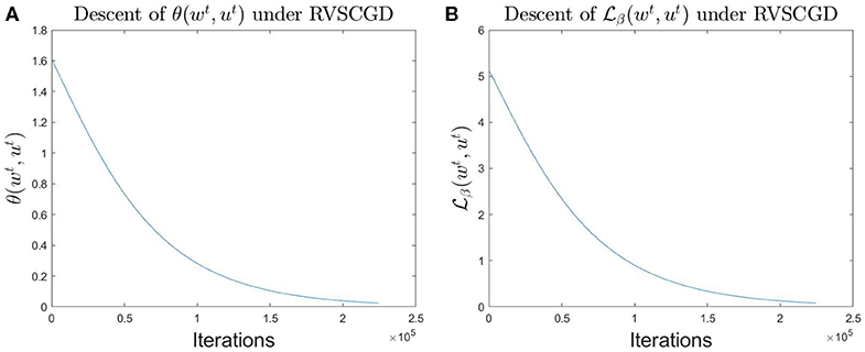
Figure 4. Behavior of θ(w^t, w^*) and ${{L}}_{\beta }(w^t,u^t)$ on the one-layer non-overlap network.

Secondly, we extend our method to a multi-layer network. Consider a variation of LeNet [47], where we replace all ReLU activations with the binarized ReLU function. The model is then trained on the MNIST dataset for 100 epochs using SGD with momentum 0.9, weight decay 5.e-4, and learning rate 1.e-3, which is decayed by a factor of 10 at epoch 60. The RVSCGD algorithm is applied on this model using the same training setting. The results are displayed in Table 1. Notice that the base model has an accuracy of 89.13%, which is lower than reported in Lecun [47]; this is because of the binarized ReLU replacement. Table 1 also shows that RVSCGD can effectively sparsify this variation of LeNet, with sparsity up to 83.76 and 4.39% loss in performance. We believe the loss in accuracy is mainly from 1-bit ReLU activation, which has too low a resolution to preserve important deep network information. We believe with higher bit quantization of weights and/or activations, networks can be more effectively pruned while still maintaining good performance (see [14]). This is a topic for our future studies.

TABLE 1

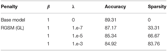
Table 1. Accuracy and sparsity of RVSCGD on a LeNet variation, on the MNIST dataset.

7. Conclusion

We introduced a variable splitting coarse gradient descent method to learn a one-hidden layer neural network with sparse weight and binarized activation in a regression setting. The proof is based on the descent of a Lagrangian function and the angle between the sparse and true weights, and applies to ℓ₁, ℓ₀ and Tℓ₁ sparse penalties. We plan to extend our work to a classification setting in the future.

Data Availability Statement

All datasets generated for this study are included in the article/supplementary material.

Author Contributions

TD performed the analysis. All authors contributed to the discussions and production of the manuscript.

Funding

The work was partially supported by NSF grants IIS-1632935 and DMS-1854434.

Conflict of Interest

The authors declare that the research was conducted in the absence of any commercial or financial relationships that could be construed as a potential conflict of interest.

Acknowledgments

This manuscript has been released as a pre-print at http://export.arxiv.org/pdf/1901.09731 [48].

References

1. Hinton G, Deng L, Yu D, Dahl GE, Mohamed A, Jaitly N, et al. Deep neural networks for acoustic modeling in speech recognition: the shared views of four research groups. IEEE Signal Process Mag. (2012) 29:82–97. doi: 10.1109/MSP.2012.2205597

CrossRef Full Text | Google Scholar

2. Krizhevsky A, Sutskever I, Hinton GE. ImageNet classification with deep convolutional neural networks. In: Bartlett PL, Pereira FCN, Burges CJC, Bottou L, Weinberger KQ, editors. Advances in Neural Information Processing Systems 25: 26th Annual Conference on Neural Information Processing Systems 2012 (2012). p. 1106–14. Available online at: http://papers.nips.cc/paper/4824-imagenet-classification-with-deep-convolutional-neural-networks

3. Dauphin YN, Fan A, Auli M, Grangier D. Language modeling with gated convolutional networks. In: Proceedings of the 34th International Conference on Machine Learning, Vol. 70. Sydney, NSW (2017). p. 933–41. doi: 10.5555/3305381.3305478

CrossRef Full Text | Google Scholar

4. Blum AL, Rivest RL. Training a 3-node neural network is NP-complete. In: José HS, Werner R, Rivest RL, editors. Machine Learning: From Theory to Applications: Cooperative Research at Siemens and MIT. Berlin; Heidelberg: Springer (1993). p. 9–28. doi: 10.1007/3-540-56483-7_20

CrossRef Full Text | Google Scholar

5. Shamir O. Distribution-specific hardness of learning neural networks. J Mach Learn Res. (2018) 19:1532–35. doi: 10.5555/3291125.3291157

CrossRef Full Text | Google Scholar

6. Tian Y. An analytical formula of population gradient for two-layered ReLU network and its applications in convergence and critical point analysis. In: Proceedings of the 34th International Conference on Machine Learning, Vol. 70. Sydney, NSW: JMLR.org (2017). p. 3404–13. doi: 10.5555/3305890.3306033

CrossRef Full Text | Google Scholar

7. Brutzkus A, Globerson A. Globally optimal gradient descent for a convnet with Gaussian inputs. In: Proceedings of the 34th International Conference on Machine Learning, Vol. 70. Sydney, NSW: JMLR.org (2017). p. 605–14.

Google Scholar

8. Zhang C, Bengio S, Hardt M, Recht B, Vinyals O. Understanding deep learning requires rethinking generalization. In: 5th International Conference on Learning Representations, ICLR 2017. Toulon (2017). Available online at: https://openreview.net/forum?id=Sy8gdB9xx

Google Scholar

9. LeCun Y, Denker J, Solla S. Optimal brain damage. In: Proceedings of the 2nd International Conference on Neural Information Processing Systems. Cambridge, MA: MIT Press (1989). p. 589–605. doi: 10.5555/109230.109298

CrossRef Full Text

10. Han S, Mao H, Dally WJ. Deep compression: compressing deep neural network with pruning, trained quantization and huffman coding. In: Bengio Y, LeCun Y, editors. 4th International Conference on Learning Representations, ICLR 2016. San Juan (2016). Available online at: http://arxiv.org/abs/1510.00149

Google Scholar

11. Ullrich K, Meeds E, Welling M. Soft weight-sharing for neural network compression. In: 5th International Conference on Learning Representations, ICLR 2017. Toulon (2017). Available online at: https://openreview.net/forum?id=HJGwcKclx

Google Scholar

12. Molchanov D, Ashukha A, Vetrov D. Variational dropout sparsifies deep neural networks. In: Proceedings of the 34th International Conference on Machine Learning, Vol. 70. Sydney, NSW: JMLR.org (2017). p. 2498–507. doi: 10.5555/3305890.3305939

CrossRef Full Text | Google Scholar

13. Louizos C, Welling M, Kingma D. Learning sparse neural networks through L₀ regularization. In: 6th International Conference on Learning Representations, ICLR 2018. Vancouver, BC (2018). Available online at: https://openreview.net/forum?id=H1Y8hhg0b

Google Scholar

14. Yin P, Zhang S, Lyu J, Osher S, Qi Y, Xin J. Blended coarse gradient descent for full quantization of deep neural networks. Res Math Sci. (2019) 6:14. doi: 10.1007/s40687-018-0177-6

CrossRef Full Text | Google Scholar

15. Daubechies I, Defrise M, Mol CD. An iterative thresholding algorithm for linear inverse problems with a sparsity constraint. Commun Pure Appl Math. (2004) 57:1413–57. doi: 10.1002/cpa.20042

CrossRef Full Text | Google Scholar

16. Candés E, Romberg J, Tao T. Stable signal recovery from incomplete and inaccurate measurements. Commun Pure Appl Math. (2006) 59:1207–23. doi: 10.1002/cpa.20124

CrossRef Full Text | Google Scholar

17. Blumensath T, Davies M. Iterative thresholding for sparse approximations. J Fourier Anal Appl. (2008) 14:629–54. doi: 10.1007/s00041-008-9035-z

CrossRef Full Text | Google Scholar

18. Blumensath T. Accelerated iterative hard thresholding. Signal Process. (2012) 92:752–6. doi: 10.1016/j.sigpro.2011.09.017

CrossRef Full Text | Google Scholar

19. Zhang S, Xin J. Minimization of transformed l₁ penalty: closed form representation and iterative thresholding algorithms. Commun Math Sci. (2017) 15:511–37. doi: 10.4310/CMS.2017.v15.n2.a9

CrossRef Full Text | Google Scholar

20. Nikolova M. Local strong homogeneity of a regularized estimator. SIAM J Appl Math. (2000) 61:633–58. doi: 10.1137/S0036139997327794

CrossRef Full Text | Google Scholar

21. Zhang S, Xin J. Minimization of transformed l₁ penalty: theory, difference of convex function algorithm, and robust application in compressed sensing. Math Program Ser B. (2018) 169:307–36. doi: 10.1007/s10107-018-1236-x

CrossRef Full Text | Google Scholar

22. Donoho D. Denoising by soft-thresholding. IEEE Trans Inform Theor. (1995) 41:613–27. doi: 10.1109/18.382009

CrossRef Full Text | Google Scholar

23. Moreau JJ. Proximité et dualité dans un espace hilbertien. Bull Soc Math France. (1965) 93:273–99. doi: 10.24033/bsmf.1625

CrossRef Full Text | Google Scholar

24. Livni R, Shalev-Shwartz S, Shamir O. On the computational efficiency of training neural networks. In: Proceedings of the 27th International Conference on Neural Information Processing Systems, Vol. 1. Cambridge, MA: MIT Press (2014). p. 855–63.

Google Scholar

25. Shalev-Shwartz S, Shamir O, Shammah S. Failures of gradient-based deep learning. In: Precup D, Teh YW, editors. Proceedings of the 34th International Conference on Machine Learning, Vol. 70. Sydney, NSW: PMLR (2017). p. 3067–75. Available online at: http://proceedings.mlr.press/v70/shalev-shwartz17a.html

Google Scholar

26. Robbins H, Monro S. A stochastic approximation method. Ann Math Stat. (1951) 22:400–7. doi: 10.1214/aoms/1177729586

CrossRef Full Text | Google Scholar

27. Rumelhart D, Hinton G, Williams R. Learning representations by back-propagating errors. Nature. (1986) 323:533–6. doi: 10.1038/323533a0

CrossRef Full Text | Google Scholar

28. Polyak B. Some methods of speeding up the convergence of iteration methods. USSR Comput Math Math Phys. (1964) 4:1–17. doi: 10.1016/0041-5553(64)90137-5

CrossRef Full Text | Google Scholar

29. Duchi J, Hazan E, Singer Y. Adaptive subgradient methods for online learning and stochastic optimization. J Machine Learn Res. (2011) 12:2121–59. doi: 10.5555/1953048.2021068

CrossRef Full Text | Google Scholar

30. Tieleman T, Hinton G. Divide the Gradient by a Running Average of Its Recent Magnitude. Technical report. Coursera: Neural networks for machine learning (2017).

31. Kingma D, Ba J. Adam: a method for stochastic optimization. In: Bengio Y, LeCun Y, editors. 3rd International Conference on Learning Representations, ICLR 2015. San Diego, CA (2015). Available online at: http://arxiv.org/abs/1412.6980

Google Scholar

32. Reddi SJ, Kale S, Kumar S. On the convergence of adam and beyond. In: 6th International Conference on Learning Representations, ICLR 2018. Vancouver, BC (2018). Available online at: https://openreview.net/forum?id=ryQu7f-RZ

Google Scholar

33. Du S, Lee J, Tian Y. When is a convolutional filter easy to learn? arXiv [preprint] arXiv:1709.06129. (2017).

Google Scholar

34. Du S, Lee J, Tian Y, Singh A, Poczos B. Gradient descent learns one-hidden-layer CNN: don't be afraid of spurious local minima. In: Dy J, Krause A, editors. Proceedings of the 35th International Conference on Machine Learning, Vol. 80. Stockholm: PMLR (2018). p. 1339–48. Available online at: http://proceedings.mlr.press/v80/du18b.html

Google Scholar

35. Courbariaux M, Bengio Y, David J-P. BinaryConnect: training deep neural networks with binary weights during propagations. In: Proceedings of the 28th International Conference on Neural Information Processing Systems, Vol. 2 (Cambridge, MA: MIT Press (2015). p. 3123–31.

Google Scholar

36. Yin P, Zhang S, Qi Y, Xin J. Quantization and training of low bit-width convolutional neural networks for object detection. J Comput Math. (2019) 37:349–59. doi: 10.4208/jcm.1803-m2017-0301

CrossRef Full Text | Google Scholar

37. Yin P, Zhang S, Lyu J, Osher S, Qi Y, Xin J. BinaryRelax: a relaxation approach for training deep neural networks with quantized weights. SIAM J Imag Sci. (2018) 11:2205–23. doi: 10.1137/18M1166134

CrossRef Full Text | Google Scholar

38. Hinton G. Neural Networks for Machine Learning, Coursera. Coursera, Video Lectures (2012).

39. Hubara I, Courbariaux M, Soudry D, El-Yaniv R, Bengio Y. Binarized neural networks: training neural networks with weights and activations constrained to +1 or −1. arXiv [preprint] arXiv:160202830. (2016).

Google Scholar

40. Cai Z, He X, Sun J, Vasconcelos N. Deep learning with low precision by half-wave Gaussian quantization. In: 2017 IEEE Conference on Computer Vision and Pattern Recognition (CVPR). Honolulu, HI (2017). p. 5406–14.

41. Taylor G, Burmeister R, Xu Z, Singh B, Patel A, Goldstein T. Training neural networks without gradients: a scalable ADMM approach. In: Proceedings of the 33rd International Conference on International Conference on Machine Learning, Vol. 48. New York, NY: JMLR.org (2016). p. 2722–31.

Google Scholar

42. Carreira-Perpinan M, Wang W. Distributed optimization of deeply nested systems. In: Kaski S, Corander J, editors. Proceedings of the Seventeenth International Conference on Artificial Intelligence and Statistics. Reykjavik: PMLR (2014). p. 10–19. Available online at: http://proceedings.mlr.press/v33/carreira-perpinan14.html

Google Scholar

43. Zhang Z, Chen Y, Saligrama V. Efficient training of very deep neural networks for supervised hashing. In: 2016 IEEE Conference on Computer Vision and Pattern Recognition (CVPR). Las Vegas, NV (2016). p. 1487–95.

Google Scholar

44. Attouch H, Bolte J, Redont P, Soubeyran A. Proximal alternating minimization and projection methods for nonconvex problems: an approach based on the Kurdyka-Lojasiewicz inequality. Math Oper Res. (2010) 35:438–57. doi: 10.1287/moor.1100.0449

CrossRef Full Text | Google Scholar

45. Wu T. Variable splitting based method for image restoration with impulse plus Gaussian noise. Math Probl Eng. (2016) 2016:3151303. doi: 10.1155/2016/3151303

CrossRef Full Text | Google Scholar

46. Wang Y, Zeng J, Yin W. Global convergence of ADMM in nonconvex nonsmooth optimization. J Sci Comput. (2019) 78:29–63. doi: 10.1007/s10915-018-0757-z

CrossRef Full Text | Google Scholar

47. Lecun Y, Bottou L, Bengio Y, Haffner P. Gradient-based learning applied to document recognition. Proc IEEE. (1998) 86:2278–324. doi: 10.1109/5.726791

CrossRef Full Text | Google Scholar

48. Dinh T, Xin J. Convergence of a relaxed variable splitting coarse gradient descent method for learning parse weight binarized activation neural network. arXiv [preprint] arXiv:1901.09731. (2019).

Google Scholar