Studying Complex Adaptive Systems With Internal States: A Recurrence Network Approach to the Analysis of Multivariate Time-Series Data Representing Self-Reports of Human Experience

Time Series of Self-Reports of Human Experience: a Complex Systems Approach

Technological advances have made collecting densely sampled physiological, behavioral, and psychological data from individuals relatively easy and inexpensive (e.g., sensors and apps on “wearables” and personal electronic devices). The availability of such large, multivariate time-series data of human physiology and well-being is of great interest to the social, behavioral, and medical sciences; however, there is at present no consensus on how to analyze such datasets or how to interpret the results obtained by different analytic approaches [1–3].

The challenges faced by researchers in these disciplines entail more than expanding their analytical toolbox of population statistics to include multivariate time-series analyses. Measurements of the temporal evolution of mental or emotional states are known as Experience Sampling or Ecological Momentary Assessment (e.g., daily ratings of “Today I feel happy” on an ordered categorical scale from 1 = “completely disagree” to 5 = “completely agree”). Analysis strategies of such datasets expose some well-known concerns about the validity of assumptions pertaining to the theoretical object of measurement and the nature of the data generating processes underlying human behavior and cognition [4–6].

Our main concerns are about the validity of the following assumptions:

1. The assumption that the ergodic theorems apply [7] to the theoretical objects of measurement and data generating processes: Ensemble averages of variables observed in samples of sufficiently many individuals are expected to be arbitrarily similar to the time averages of variables evolving over a sufficiently long interval of time, from any single initial condition.

2. The assumption that the interpretation of outcomes of psychological measurement is, or, should be, equivalent to classical physical measurement [8]: It is considered unproblematic to interpret a measurement outcome as a property of the theoretical object of measurement confounded by sources of random, additive, measurement noise, or sampling error.

The assumptions related to ergodicity (i.e., stationarity and homogeneity of central moments) are obviously important for making valid statistical inferences and generalizations. A common practice in psychopathology studies in which the Gaussian Graphical Model (GGM) is fitted to multivariate self-report data to estimate so-called “symptom networks” [9] is the use of rather ad hoc methods to achieve data reduction. For example, subsets of the multivariate time-series data are combined by simply taking their average or by using techniques like principal component analysis and exploratory factor analysis to achieve dimension reduction by estimating the network on the extracted component or factor structure. Such aggregation methods are known to be problematic if the assumptions of independence, stationarity, and homogeneity are violated [7, 10].

Even if the core assumptions for an ergodic data generating process formally apply, one cannot rely on parameter estimates to converge on a characteristic expected value within the time scale of observation or magnitude of fluctuation. This occurs for example when the process samples from a stable distribution with one or more undefined central moments like the Cauchy distribution. This has led some scholars to suggest that “the very notion of probability may not make sense” [11] when studying complex systems with internal state dynamics. Recent observations of discrepancies between inferred statistical properties at the ensemble level (inter-individual) and the individual level (intra-individual), have been suggested as a cause of the so-called reproducibility crisis in the social and life sciences [11–13]. A study that observed a lack of “group-to-individual generalizability” in the context of psychopathology described the phenomenon as a threat to human subjects research: “In clinical research, diagnostic tests may be systematically biased and our classification systems may be at least partially invalid. In terms of theory development, we may have a misleading impression about the nature of psychological variables and their interactions” [13]. A study of the neuroanatomical phenotypes of schizophrenia and bipolar disorder [14] concluded: “This study found that group-level differences disguised biological heterogeneity and interindividual differences among patients with the same diagnosis. This finding suggests that the idea of the average patient is a non-informative construct in psychiatry that falls apart when mapping abnormalities at the level of the individual patient.”

The second concern is about the lack of a clear notion of how to incorporate the measurement context and the act of measurement of psychological variables into the description of a phenomenon [15]. It seems uncontroversial to suggest that the very act of asking someone to project their current internal state of happiness onto an arbitrary ordinal scale will interfere with their “true” state of happiness (if such a thing even exists without the measurement context). However, this actually implies that psychological measurement cannot be regarded as classical physical measurement, because the outcomes of self-reports emerge as the result of an interaction between the theoretical object of measurement and the measurement context. This causes measurement problems that are at least conceptually related to contemporary discussions about the ontological status of measurement in physics [16]. Resolutions have been proposed for measurement of psychological variables, for example, various types of conjoint measurement [8, 17] or measurement models based on contemporary particle physics [15, 18, 19]. When the temporal evolution of internal states is concerned, additional issues arise due to the fact that living systems are subject to aging (loss of identity over time) and appear to be able to coordinate their current behavior relative to some record of previously experienced events (i.e., memory). In more general terms, the behavior of a complex adaptive system will display after-effects of interactions with its internal or external environment that extend far beyond any time scale that might be understood as a simple stochastic process with autoregressive components [10, 20]. Time series of observables of living systems will often lack the memoryless-ness property [21, 22], suggesting that, at least, anomalous rather than normal diffusion processes should be considered as a model for the data generating process [23].

Addressing (Some) Concerns: Recurrence Networks of Change Profiles

In the present paper, we discuss the benefits and challenges of considering multivariate time-series data that represent self-reports of human experience as the observables of a complex dynamical system with internal state dynamics (internal degrees of freedom). More specifically, we will consider the framework of (multiplex) recurrence networks [24, 25] as the preferred analytic toolbox for describing the dynamics of multivariate time series collected using the Experience Sampling Method. Recurrence networks have been used to analyze multivariate physiological data, like human EEG [26]. A publicly available dataset will be used in which four participants evaluated six questions about their self-esteem and attitudes toward their physical self, twice a day, during 512 consecutive days [27]. Figure 1 displays the time series for each participant and each variable; the ratings were evaluated on a visual analog scale, and participants moved a slider between the values 0 and 10. The analyses in the original study revealed the presence of long-range dependence, power-law scaling in virtually all cases close to 1/f noise [27]. Most time series are obviously non-stationary with respect to level and trend; some appear to reveal clear transitions between dynamical regimes, such as periods of low and high variability in responses.

FIGURE 1

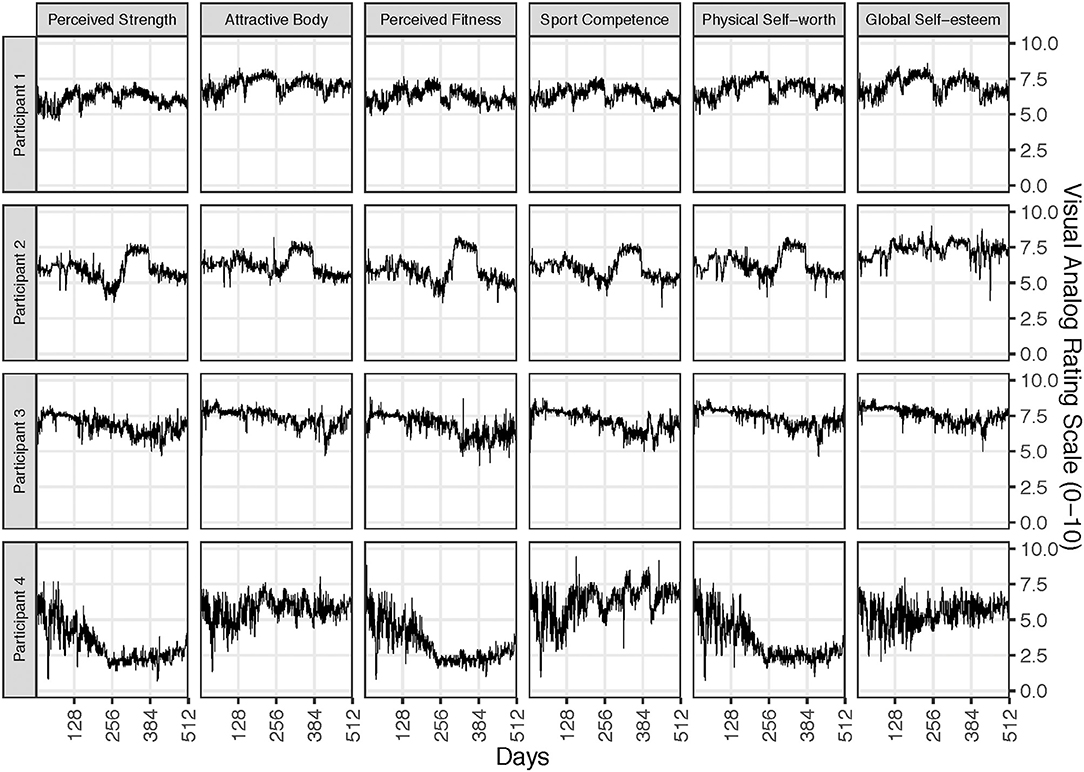
Figure 1. Bi-daily ratings of self-esteem and perception of the physical self by four participants over the course of 512 days. The data were originally reported by Delignieres et al. [27].

There are several advantages of using recurrence-based methods for time-series analysis over statistical models that require stationarity and (conditional) independence like the GGM [9], but also over models that can handle non-stationary signals like Time Varying Auto Regressive models (TV-AR) [28]. These models generally limit estimating temporal dynamics to the linear domain, and to very short time scales (e.g., lag-1 vector autoregression [9]), which severely limits the range of potential data generating processes that can be considered to underlie the observed series.

In general, recurrence analytic approaches to time-series analysis are as follows:

• Essentially model-free and make few assumptions about the data [29].

• Describe linear as well as non-linear dynamical phenomena [25].

• Describe (transitions between) dynamical regimes, even in exceptionally noisy environments [30].

• Quantify recurrent dynamics across all available time scales [25, 31].

• Quantify structural similarities between different time series represented as multiplex recurrence networks [24], suspending the need for potentially problematic aggregation and/or dimension reduction of multivariate time-series data.

By using recurrence-based methods, most of the concerns related to the assumption of ergodicity are addressed to the extent that one is able to quantify dynamical behavior associated with local ergodicity breaking. However, the concerns about the interpretation of measurement outcomes of EMA data remain, which is why we propose to transform the data prior to analysis.

In the context of the current paper, we can expect the temporal evolution of self-reported ratings of internal states projected onto an arbitrary ordinal scale to be affected by at least three factors. First, current ratings are likely evaluated relative to some moving average of previous ratings (memory). People might recall their evaluations of a couple of days ago, perhaps a week, but it is less likely they will recall the previous month and use it as a reference level. Second, changes in the function that projects the internal state onto the ordinal scale (observed as sudden shifts in level, trend, or variance) are expected to be unpredictable and nonlinear. For example, a sudden re-evaluation of the relation between internal state and values of the rating scale might be triggered by the occurrence of an event that is extreme in the sense that the scale boundaries no longer adequately represent the current state relative to previously experienced states. The projection of “Today I feel sad” onto a scale of 1–5 might change dramatically relative to previous evaluations due to the sudden loss of a loved one. Finally, it is unlikely that using the same arbitrary scale to simultaneously measure two or more different internal states within the same individual will yield projection functions that are approximately equivalent for each distinct state or that such projections will be affected in an equivalent way by the state history and experience of extreme events. Based on these assertions, we assume that the way in which the ratings change from one moment to the next relative to some (non-stationary) level is more informative than the sequence of absolute values of the scale itself. For example, in Figure 1, Participants 1, 2, and 3 stay within a very limited range of the values allowed for by the scale, but analyses reveal that these bounded fluctuations are not random at all, but represent a complex pattern of long-range dependence.

We suggest to use a change profile (CP) whenever the raw data consist of time series of self-reports on bounded ordinal scales. This transformation of the data takes the cumulative sum of deviations of observed values from an estimate of the reference level used to evaluate the current state. One could, for example, use a simple moving average in a sliding window (a linear filter) to represent the reference level. The window size should be a reasonable estimate of the lag of time across which a person's current ratings are still affected by their previous ratings. Such a lag could be estimated using a partial autocorrelation function (first lag with non-significant autocorrelations), a lagged mutual information function (e.g., lag at the first or global minimum), or a lag that makes sense based on theoretical and empirical knowledge of the process in question. Here, we consider a CP based on a running average in a right-aligned window.

The CP is a simple extension of the global profile (GP), which is obtained by first subtracting the mean of the time series from each observed value and subsequently taking the cumulative sum:

$\begin{array}{ll}G{P}_j={\displaystyle \sum _{i=1}^j}{x}_i-\overline{x},\text{ for j}=1,2,\dots ,\text{N}& (1)\end{array}$

In Equation 1, GP_j is the global profile of x_i, a time series of i = 1, …, N equidistant observations, $\overline{x}$ represents the time-series mean $\frac{1}{N}\sum _{i=1}^N{x}_i$. The main difference between the GP and CP is that instead of subtracting the constant $\overline{x}$, a running average series ${\overline{w}}_j$ calculated in a window of size W is used:

$\begin{array}{ll}{\overline{w}}_j=\frac{1}{W}{\displaystyle \sum _{i=0}^{W-1}}{x}_{i+j},\text{ with j }=1,2,\dots ,\text{N}-\text{W}& (2)\end{array}$

CP_j in Equation 3 is the cumulative sum of the differences between x_i and ${\overline{w}}_j$, but because ${\overline{w}}_j$ is a shorter sequence than x_i, one can choose how to align the two series. Using a left-aligned window refers to the differences taken starting at x_{i = 1}, in a centered window at x_{i = W/2}, and in a right-aligned window at x_{i = W}. Equation 3 represents a right-aligned window:

$\begin{array}{ll}C{P}_j={\displaystyle \sum _{i=0}^{j-1}}{x}_{i+W}-{\overline{w}}_j,\text{ with j }=1,2,\dots ,\text{ N}-\text{W}& (3)\end{array}$

Figure 2 displays the CPs for the observed variable Perceived Fitness for each participant, in which the window size was W = 14 (corresponding to 7 days). The effect of calculating the CP is that any changes in the state evaluation relative to the rolling average are “exaggerated”; the description of the state dynamics is no longer bounded by the range of the ordinal rating scale (see the Supplementary Material for a more detailed description of the effect of window size on the CP). The observed series of Participant 1, for example, oscillate around a rather stationary level in the first half of the observation period, but displays a downward trend in the second half. This can also be seen in the series of Participants 3 and 4. The CPs indicate that the dynamics driving these downward trends are likely more diverse than what might be expected based on the fluctuations of observed values on the bounded ordinal scale. In subsequent analyses that quantify recurrent states, values that are similar in the observed bounded series will be dissimilar in the unbounded CP, which we believe to be more realistic given the context of self-reports of emotional and psychological states.

FIGURE 2

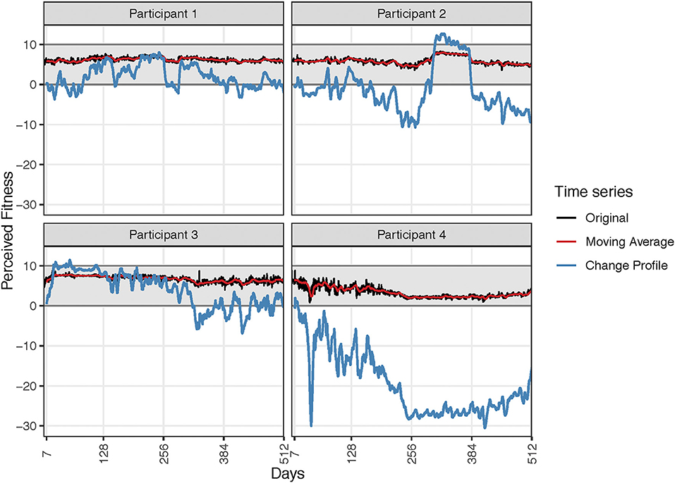
Figure 2. Change Profiles (blue lines) of the variable Perceived Fitness for each participant. The profiles were calculated using a right aligned window of 14 data points, representing 7 days (see Equation 1).

The remainder of this paper is structured as follows: In Section Weighted Recurrence Network Analysis: Recurrence Times as Edge Weights, we construct recurrence networks from the CPs of the time series in Figure 1 and discuss a method for extracting a scaling exponent from a weighted recurrence network that is similar to scaling exponents obtained from fractal analysis techniques. In Section Swing on a Spiral: A Sequential Layout for Recurrence Networks, we present novel layouts for recurrence networks designed to provide insight into the occurrence of regime shifts and network measures within certain epochs. In Section Multiplex Weighted Recurrence Networks, we construct multiplex recurrence networks and evaluate multilayer mutual information based on similarities between the strength distributions of the layers in the network.

Weighted Recurrence Network Analysis: Recurrence Times as Edge Weights

The goal of the original study reporting on the multivariate time series of the four participants in Figure 1 was to quantify the temporal structure of fluctuations in self-esteem ratings in terms of scaling exponents [27]. The results showed that all subjects produced time series that resemble long-memory processes that resemble 1/f noise. In this section, we explore whether recurrence networks can be used to extract similar information about the data, by creating networks that represent information about recurrent states as well as information about the frequency with which they occur.

To the best of our knowledge, this approach is different from previous studies using, e.g., the degree distribution (k-spectrum [32]), the transitivity, or clustering dimension to quantify dimension characteristics [24]. Weighted recurrence networks have been constructed based on multivariate EEG data [26], by creating a joint recurrence matrix (from the recurrence matrices of simultaneously recorded EEG channels). The joint recurrence rates (RRs) served as the edge weights. We propose using recurrence times as edge weights. This allows for a comparison of the scaling relation between the vertex degree k_i and vertex strength s_i (sum of the number of edges times edge weights) [33]. It has been shown that, absent any correlations between edge weights and vertex degree, the average strength of vertices of degree k scales with k as s(k) ~ k^βwith β = 1. Any deviations from β = 1 can be interpreted to arise from systematic dependencies between the edge weights and vertex degree. In the case of a recurrence network weighted by recurrence times, a scaling relation β > 1 represents the case in which the mean recurrence time of an observed state increases exponentially with the frequency with which an observed state will recur, relative to a randomly connected network. We will refer to the slope β as the recurrence rate–recurrence time dependency (irrespective of whether frequency or duration is used), abbreviated as β_RR~RT.

Weighted Recurrence Network Construction

For each participant, we constructed distance matrices by delay embedding [34] the CPs of the six self-esteem variables using a window size of 14 (7 days). We chose a common delay τ and embedding dimension m for all six time series observed within a participant, using the median of the six τ values (found as first local minima of the lagged mutual information function) and the maximum of the six embedding dimensions (found by false nearest neighbor analysis [25, 35, 36]). Settling on one set of parameters for all variables observed within an individual is necessary for the construction of a multiplex network for each participant (see Section Multiplex Weighted Recurrence Networks), which requires the same number of vertices for each layer of the network [24]. Figure 3A (created with R package casnet [37]) displays the distance matrix of the delay-embedded CP of Perceived Strength for Participant 1. To turn the distance matrix into a recurrence plot (RP, Figure 3B), which is a visualization of the recurrence matrix R_i,j, a threshold value ε is chosen. The color bar in Figure 3A represents the range of distance values in the matrix. On the right side of the color bar, distance values are reported that would result in the RR reported on the left side of the color bar, should they be chosen as the threshold value. In the present paper, we chose ε such that RR would be 5% for all R_i,j, denoted as ε_.05 in Equation 4:

$\begin{array}{ll}{R}_{i,j}({\epsilon }_{.05})=\Theta \left({\epsilon }_{.05}-\Vert {\vec{x}}_i-{\vec{x}}_j\Vert \right),i,j=1,\dots ,N& (4)\end{array}$

FIGURE 3

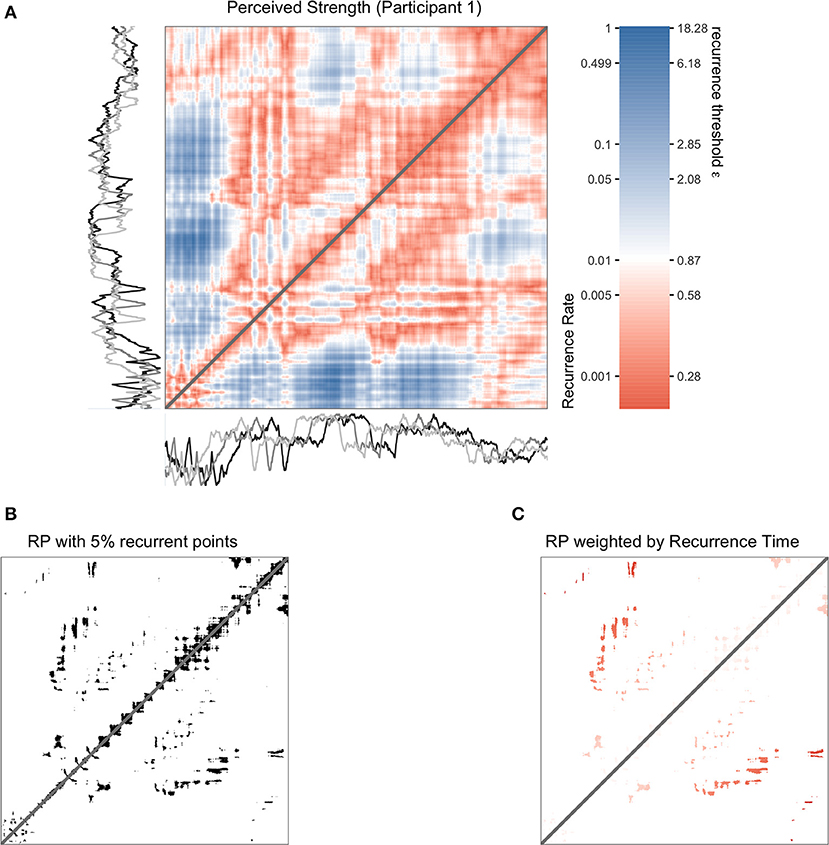
Figure 3. (A) shows a distance matrix for the Change Profile of Perceived Strength of Participant 1. The series was embedded with parameters, m = 3 and τ = 37. (B) is a recurrence matrix, a threshold value ε = 2.08 was chosen to yield RR = 0.05. A weighted recurrence matrix is shown in (C), created by eliminating all values above the threshold of ε = 2.08 and replacing the distance values with recurrence times.

The RP in Figure 3B was constructed with ε_.05 = 2.08, with N as the length of the state space vectors (series length − (m − 1) · τ), Θ as the Heaviside function (returning 0 if the distance exceeds ε_.05, 1 otherwise), and ‖ ‖·‖ ‖ as the Euclidean norm. To create a version of R_i,j weighted by recurrence time, the result of the Heaviside function (0 or 1) is multiplied by the temporal separation between two state coordinates (Figure 3C):

$\begin{array}{ll}{R}_{i,j}({\epsilon }_{.05})=\Theta \left({\epsilon }_{.05}-\Vert {\vec{x}}_i-{\vec{x}}_j\Vert \right).|i-j|,i,j=1,\dots ,N& (5)\end{array}$

If a time stamp is available, the weights |i − j| can be expressed as a duration in the observed units of time. For the purpose of comparing the strength-degree scaling relation s(k) ~ k^β to the scaling relation between frequency and power obtained from a power spectrum of the time series, we represent the weights as a frequency $\frac{1}{|i-j|}$.

Power-Law Scaling in Time Series and Weighted Networks

First, we study how the scaling relation s(k) ~ k^β (in the present context with β_RR~RT) behaves when we create weighted recurrence networks of simulated ideal colored noise series. Time series were generated using a procedure based on the inverse Fourier transform that allows constructing a specific scaling relation between frequency and power in the frequency domain (a log–log slope in Power Spectral Density, see [38]). Figure 4A displays a set of 51 simulated time series of which the PSD slope varies from −2.5 to 2.5 in 0.1 increments; that is, noises include Brownian (red) noise (−2) to pink (−1), white (0), blue noise (1), and violet noise (2). For each of the 51 scaling relations, we generated 100 noise series (each with different random seeds) and created recurrence networks, choosing the delay τ and embedding dimension m as described in the previous paragraph (see Table 1).

FIGURE 4

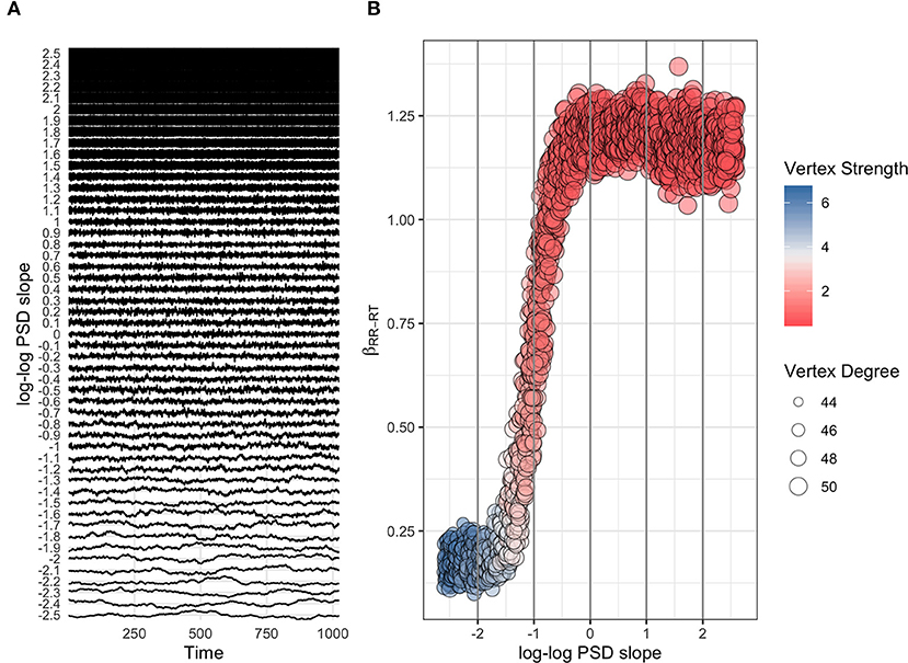
Figure 4. (A) shows one set of 51 (out of 100) simulated ideal noise series with log–log PSD slopes varying between −2.5 and 2.5. (B) represents the relation between the log–log PSD slopes and β_RR~RT. Each of the 5,100 circles represents a recurrence network constructed from a simulated noise series. Circles are color coded according to the mean vertex strength s(k), and their size represents the mean vertex degree k. The Spearman correlation between log–log PSD slopes in the range [−2,0] and β_RR~RT is 0.93.

TABLE 1

Table 1. Mean and standard deviation (SD) of the embedding parameters and recurrence network measures for the simulated series in Figure 4.

A threshold ε was selected that yielded a 5% RR. This means the average vertex degree of each network will be approximately the same, but will vary with the length of the embedded series. Figure 4B shows the relation between β_RR~RT of each recurrence network and the log–log PSD slope from the simulated series from which it was constructed. The plot suggests a logistic relation, which has an almost perfect linear relationship (r_S = 0.93) for noise series with log–log PSD slopes in the range of [−2, 0]. Outside of this range, the β_RR~RT slope does not seem to be able to distinguish very well between log–log PSD slopes; the Spearman correlation for the full range is r_S = 0.75. Another interesting pattern that can be seen in Figure 4B is that the highest mean vertex strengths are associated with negative log–log PSD slopes (r_S = −0.94), whereas the highest average vertex degrees are associated with positive log–log PSD slope (r_S = 0.85).

Compared to the observed series in Figure 1, the simulated series are relatively stationary, homogeneous, and void of noise. When the scaling relation β_RR~RT is calculated based on the observed data (Figure 5), we arrive at the same conclusion as the original study [27]: These observed time-series display a structure of temporal dependencies that resembles the category of colored noises between pink noise (PSD slope −1) and red noise (PSD slope −2). Table 2 displays the values of β_RR~RT and the estimated log–log PSD slope for each participant and variable. In addition, we use the linear relationship for log–log PSD slope ranges of [−2, 0] to predict the log–log PSD slope from β_RR~RT, which is approximately: PSD slope ≈ −1.94 + 1.38 · β_RR~RT. As can be seen in the final row of Table 2, the deviation between the predicted and estimated PSD slope is rather small on average.

FIGURE 5

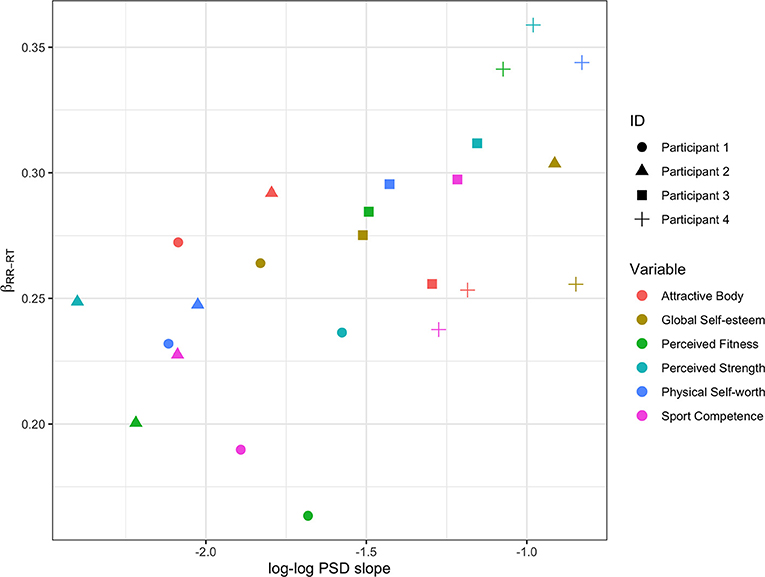
Figure 5. The relation between the log–log PSD slopes and β_RR~RT for each participant and each observed variable.

TABLE 2

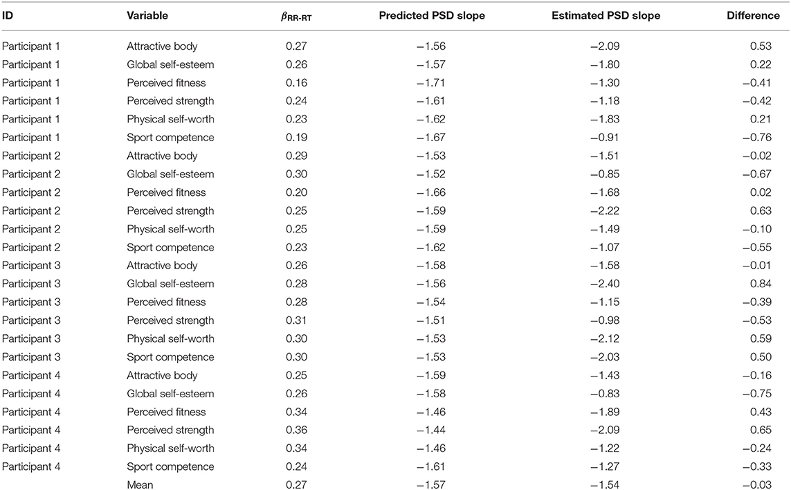
Table 2. Relation between β_RR−RT, predicted PSD slope, and estimated PSD slope for each participant and variable.

Swing on a Spiral: a Sequential Layout for Recurrence Networks

Graphical representations of recurrence networks often use layouts that emphasize certain structural properties (e.g., “spring” layouts) and discard information about the temporal order, the vertex sequence. However, in a clinical setting, e.g., if multivariate time-series data are used to detect imminent regime shifts, such as sudden gains and losses in symptom severity [39, 40], it is important to retain temporal information. Here, we present a simple layout for recurrence networks based on the spiral. Figure 6 displays a basic Archimedean spiral layout in which the vertices are equally divided over six arcs. The edge weights are set to the recurrence time frequency. The RN represents the CP of the variable Perceived Strength produced by Participant 1 and weighted by recurrence time.

FIGURE 6

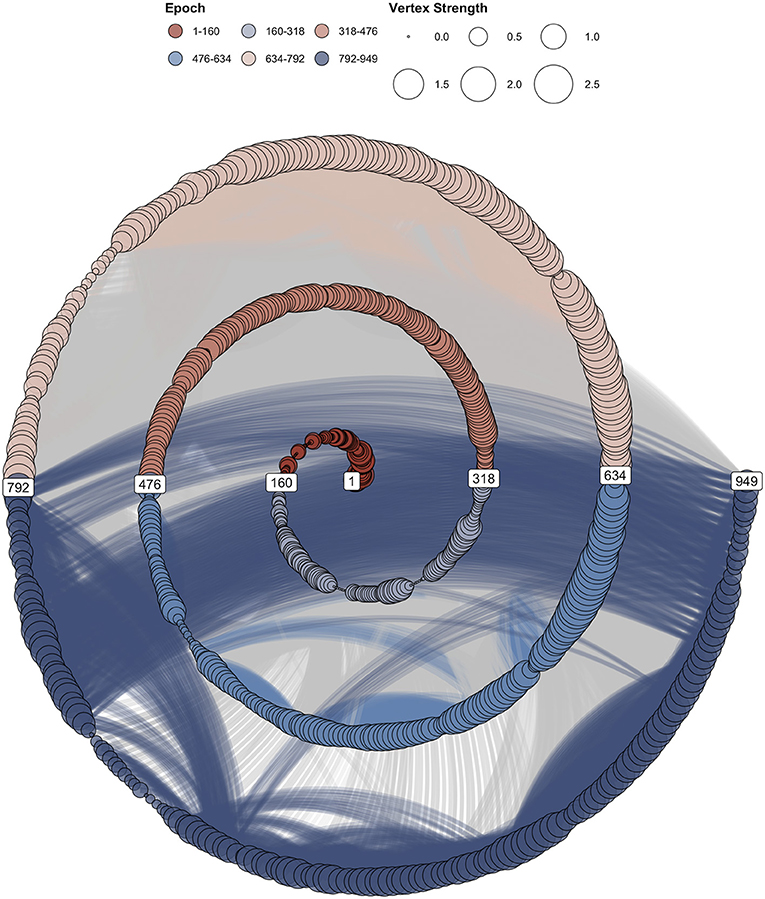
Figure 6. A spiral layout of the recurrence network of the change profile of variable Perceived Strength produced by Participant 1. Edges with recurrence times of 10 or smaller (5 days) were removed to improve visibility.

In Figure 6, each arc corresponds to an epoch, which is color coded, but epochs could also describe months, years, phases in an experiment, or other qualitative descriptors of segments of time. If edges connect vertices within the same epoch, they are represented in the vertices; otherwise, they are gray (see the Supplementary Material for spiral RNs of each participant and each variable in the dataset). This provides a rough indication of differences between longer and shorter recurrence times.

Although the estimated scaling exponents of the time series for each participant fall within a similar range [27], Figure 7 shows that the recurrence network on a spiral suggests that the power laws arise from rather different patterns of recurrent states, occurring at different moments in time. The RN of Participant 3 reveals lots of recurrent states in the first two arcs, and very few later on in the time series, whereas the RN of Participant 4 indicates most recurrent states occurring in the final arc and across different arcs (longer recurrence times). It is possible to change the spiral layout to highlight different structural aspects of the RN.

FIGURE 7

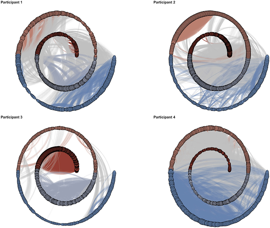
Figure 7. Spiral graphs with four arcs of the variable Global Self-Esteem for each participant. Edges with recurrence times of 10 or smaller (5 days) were removed to improve visibility.

Figure 8 shows a number of different layout options for the CP of Participant 3 in Figure 7. The Archimedean spiral (top left) in Figure 8 is similar to the layout in Figures 6, 7, except for the start and end of the time series, which are reversed. In Archimedean spirals, points on the spiral that intersect a line going through the origin will all be equidistant. This means the first part instead of the last part of the time series will be emphasized if the order is reversed, because it is now displayed on the longest arcs of the spiral. In the Bernoulli and Fermat spiral layout (Figure 8, top right and bottom left), the length of the arcs increases with each turn, which emphasizes the part of the series represented on the outer arcs. The Euler spiral layout can emphasize the middle part of the time series.

FIGURE 8

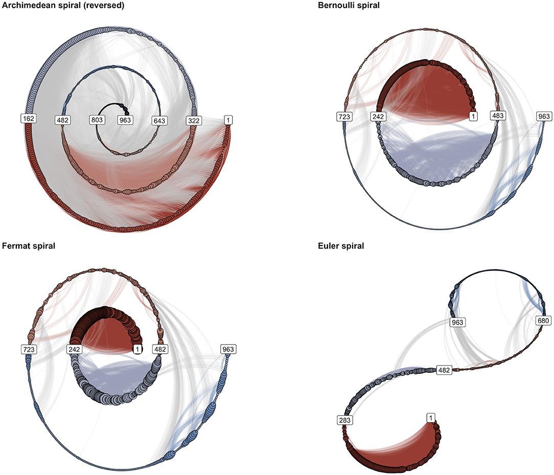
Figure 8. A showcase of spiral graphs using the variable Global Self-Esteem of Participant 3 in Figure 7. Each spiral type (Archimedean, Bernoulli, Fermat, and Euler) can highlight different aspects of the temporal structure of recurrent states. Edges with recurrence times of 10 or smaller (5 days) were removed to improve visibility.

Multiplex Weighted Recurrence Networks

Multiplex recurrence networks provide a framework for studying the temporal structure in multivariate time series. To obtain a multiplex weighted recurrence network (MwRN), we simply consider the six recurrence time frequency weighted RNs for each participant as the layers of a larger network, the MwRN. The structural association between layers α and β in an unweighted MRN can be quantified by the interlayer mutual information measure I_α,β that is based on the degree distributions P(κ^[α]), P(κ^[β]) of the vertices in each layer [41, 42]:

$\begin{array}{ll}{I}_{\alpha ,\beta }={\displaystyle \sum _{{\kappa }^{[\alpha ]}}}{\displaystyle \sum _{{\kappa }^{[\beta ]}}^{}}P\left({\kappa }^{[\alpha ]},{\kappa }^{[\beta ]}\right).log\frac{P\left({\kappa }^{[\alpha ]},{\kappa }^{[\beta ]}\right)}{P\left({\kappa }^{[\alpha ]}\right)P\left({\kappa }^{[\beta ]}\right)}& (6)\end{array}$

The term P(κ^[α], κ^[β]) denotes the joint probability of observing the same vertex with degree κ^[α] in layer α and degree κ^[β] in layer β. P(κ^[α]) and P(κ^[β]) represent the marginal probabilities of observing the degree distribution in each layer.

Taking I_α,β as the weight between two layers in a multiplex network can be interpreted as the quantification of structural regularities between the time series in the multivariate dataset. This is of course a more abstract-level interpretation of the mutual information quantity: The averaged mutual information across all layers, I_α,β, in a multiplex network can be interpreted as a quantification of typical information flow between the dimensions of the multivariate system [41, 42].

For the weighted RNs, we construct a multilayer mutual information based on the strength distributions in each layer, e.g., $P\left({s}{\left(k\right)}^{\left[\alpha \right]}\right),P\left({s}{\left(k\right)}^{\left[\beta \right]}\right)$, by simply exchanging vertex degree for vertex strength:

$\begin{array}{ll}{I}_{\alpha ,\beta }={\displaystyle \sum _{{s}{\left(\kappa \right)}^{\left[\alpha \right]}}{\displaystyle \sum _{{s}{\left(\kappa \right)}^{\left[\beta \right]}}P\left({s}{\left(\kappa \right)}^{\left[\alpha \right]},{s}{\left(\kappa \right)}^{\left[\beta \right]}\right)}}\cdot log\frac{P\left({s}{\left(\kappa \right)}^{\left[\alpha \right]},{s}{\left(\kappa \right)}^{\left[\beta \right]}\right)}{P\left({s}{(\kappa )}^{\left[\alpha \right]}\right)P\left({s}{(\kappa )}^{\left[\beta \right]}\right)}& (7)\end{array}$

Figure 9 displays the MwRNs for each participant; the edges connecting a layer α and β represent the mutual information I_α,β based on the vertex strength distribution in those layers. I_α,β can be said to quantify the typical information flow between the layers of the MwRN; in the present case, this can be interpreted as the characteristic way in which self-reports of internal states related to self-esteem and physical self-worth are associated across time scales spanning from half a day to 512 days. Different patterns of similar structure can be identified among participants. The MwRN of Participant 3 reveals that associations between Global Self-Esteem, Physical Strength, and Perceived Fitness are highest, whereas the strongest structural similarities in the MwRN of Participant 4 occur between the layers Global Self-Esteem, Sport Competence, and Attractive Body. Participants 1 and 2 show more diverse flow patterns. In Table 3, several MwRN measures were reported: The Layer Strength for each layer in the MwRN, which in the present case is just the number of layers times the value of I_α,β (the vertex degree is always 6, because we did not impose a threshold to remove edges). The Average Edge Overlap measure represents the proportion of edges that are shared between any two vertices across all layers [42]. The average I_α,β is simply the mean of the edge weights.

FIGURE 9

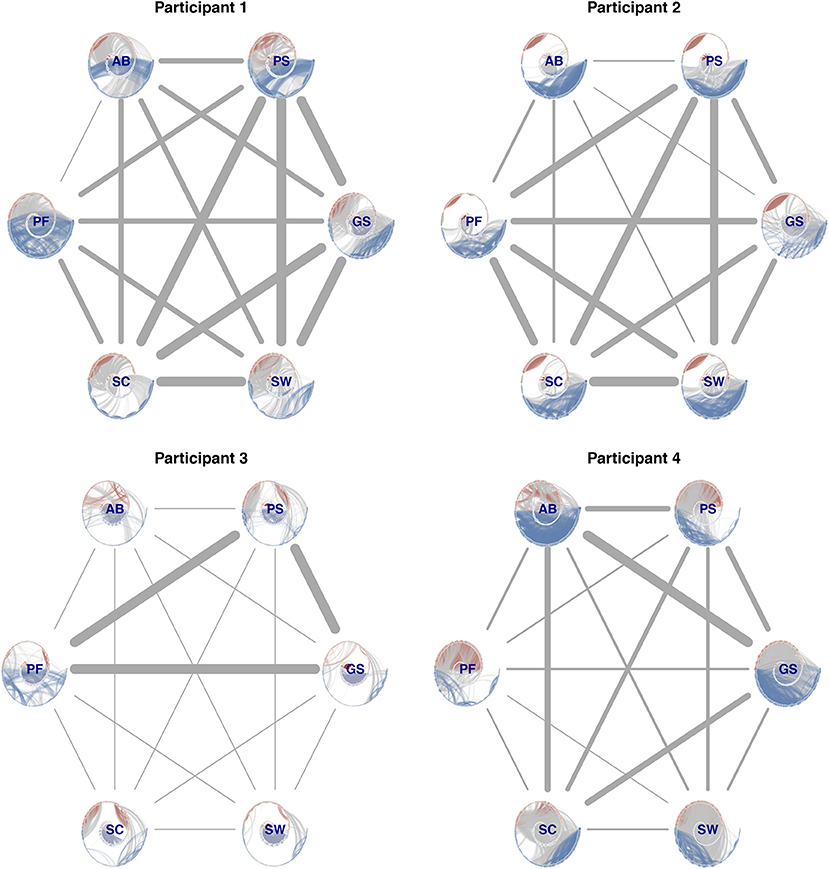
Figure 9. Multiplex weighted recurrence networks for each multivariate dataset. The layers of the network represent the RNs of the observed change profiles (AB, Attractive Body; PS, Physical Strength; GS, Global Self-Esteem; SW, Physical Self-Worth; SC, Sport Competence; PF, Perceived Fitness). The edge weights represent the multilayer mutual information, I_α,β, based on the strength distribution in each layer.

TABLE 3

Table 3. Layer strength, average edge overlap, and multilayer mutual information of the MwRNs in Figure 9.

Conclusion and Discussion

A primary goal of the present paper was to address some of the issues that arise when multivariate time series of self-reports of human experience are analyzed and interpreted under the assumption that:

1. The data generating process is essentially stationary, homogeneous, and void of long-range dependencies.

2. The measurement process can be considered classical physical measurement.

We explored a publicly available dataset of which it is known that the multivariate time series represent non-stationary data with long-range dependence [27].

First, we showed that focusing on how internal states change relative to a non-stationary reference level, the CP seems to be a more sensible observable than the sequence of values allowed for by the arbitrary ordinal rating scale. A secondary goal was to show that analytic methods developed to study complex adaptive systems can be applied to time series of self-reports of human experience (EMA data) and that the results can be sensibly interpreted and visualized. We were able to construct recurrence networks using regular methods for delay-embedding time series (mutual information, false nearest neighbor analysis). Moreover, we study recurrence networks weighted by recurrence time (or recurrence time frequency) and show that a scaling relation β_RR~RT can be estimated that is very similar to the scaling relation estimated from the power spectrum, for a specific range of scaling exponents [−2,0].

Many of the potential applications of recurrence networks to EMA data would benefit from a visualization of the network in which the temporal order of observed values is retained and we suggest that the spiral layout might be beneficial in this respect. Finally, we constructed multilayer recurrence networks that revealed that characteristic patterns of fluctuations in self-reports about self-esteem vary across participants and reveal a limited subset of variables sharing similar structure over time in some participants, whereas other participants appear to share structure in temporal dynamics that include almost all observed variables. Of course, the present study is in fact “merely” a multiple case study, and more research will be required in order to decide whether the approach presented here generalizes to other datasets as well. We do believe that the present paper provides at least a proof of principle with respect to the applicability of the recurrence network approach to EMA data, which can potentially be a valuable analytic method for idiographic research, especially in psychopathology.

To summarize, we suggest that using a recurrence-based approach to analyze multivariate time-series data that can be considered to emerge from a complex adaptive system with internal state dynamics should be preferred over analytic methods that attempt to fit the parameters of a statistical model. The data generating processes underlying the multivariate series will almost certainly violate the key assumptions of stationary and homogeneity, and likely do not possess the memoryless-ness property.

Data Availability Statement

The datasets analyzed for this study can be found on the website of the first authors of the original publication [27]: https://didierdelignieresblog.wordpress.com/recherche/databank/.

Author Contributions

FH conceived of hypotheses, methods, analyses, and structure. FH and AB wrote the article.

Funding

This article was written while FH was employed by the School of Pedagogical and Educational Sciences at the Radboud University.

Conflict of Interest

The authors declare that the research was conducted in the absence of any commercial or financial relationships that could be construed as a potential conflict of interest.

Supplementary Material

The Supplementary Material for this article can be found online at: https://www.frontiersin.org/articles/10.3389/fams.2020.00009/full#supplementary-material

References

1. Shiffman S. Conceptualizing analyses of ecological momentary assessment data. Nicotine Tob Res. (2014) 16 (Suppl. 2):S76–87. doi: 10.1093/ntr/ntt195

PubMed Abstract | CrossRef Full Text | Google Scholar

2. Nezlek J. Ecological momentary assessment: statistical issues. Eur Psychiatry. (2015) 30:121. doi: 10.1016/S0924-9338(15)31837-X

CrossRef Full Text | Google Scholar

3. Conner TS, Tennen H, Fleeson W, Barrett LF. Experience sampling methods: a modern idiographic approach to personality research. Soc Personal Psychol Compass. (2009) 3:292–313. doi: 10.1111/j.1751-9004.2009.00170.x

PubMed Abstract | CrossRef Full Text | Google Scholar

4. Bringmann LF, Elmer T, Epskamp S, Krause RW, Schoch D, Wichers M, et al. What do centrality measures measure in psychological networks? J Abnorm Psychol. (2019) 128:892–903. doi: 10.1037/abn0000446

PubMed Abstract | CrossRef Full Text | Google Scholar

5. Molenaar PCM. Consequences of the ergodic theorems for classical test theory, factor analysis, and the analysis of developmental processes. In: Hofer SM, Alwin DF, editors. Handbook of Cognitive Aging: Interdisciplinary Perspectives. Thousand Oaks, CA: SAGE Publications, Inc. (2008). p. 90–104.

Google Scholar

6. van Bork R, Rhemtulla M, Waldorp LJ, Kruis J, Rezvanifar S, Borsboom D. Latent variable models and networks: statistical equivalence and testability. Multivariate Behav Res. (2019) 16:1–24. doi: 10.1080/00273171.2019.1672515

CrossRef Full Text | Google Scholar

7. Molenaar PC. On the implications of the classical ergodic theorems: analysis of developmental processes has to focus on intra-individual variation. Dev Psychobiol. (2008) 50:60–9. doi: 10.1002/dev.20262

PubMed Abstract | CrossRef Full Text | Google Scholar

8. Luce RD, Narens L. Symmetry, scale, types, and generalizations of classical physical measurment. J Math Psychol. (1983) 27:44–85. doi: 10.1016/0022-2496(83)90026-3

CrossRef Full Text | Google Scholar

9. Epskamp S, Cramer AOJ, Waldorp LJ, Schmittmann VD, Borsboom D. qgraph: Network visualizations of relationships in psychometric data. J Stat Softw. (2012) 48:1–18. doi: 10.18637/jss.v048.i04

CrossRef Full Text | Google Scholar

10. Beran J. Statistical methods for data with long-range dependence. Stat Sci. (1992) 7:404–16. doi: 10.1214/ss/1177011122

CrossRef Full Text | Google Scholar

11. Press WH. Reproducibility Now at Risk? Symposium on Evidence in the Natural Sciences 30-05-2014. New York, NY: Simons Foundation (2014).

12. Wallot S, Kelty-Stephen DG. Interaction-dominant causation in mind and brain, and its implication for questions of generalization and replication. Minds Machines. (2017) 28:353–74. doi: 10.1007/s11023-017-9455-0

CrossRef Full Text | Google Scholar

13. Fisher AJ, Medaglia JD, Jeronimus BF. Lack of group-to-individual generalizability is a threat to human subjects research. Proc Natl Acad Sci USA. (2018) 115:E6106–E15. doi: 10.1073/pnas.1711978115

PubMed Abstract | CrossRef Full Text | Google Scholar

14. Wolfers T, Doan NT, Kaufmann T, Alnaes D, Moberget T, Agartz I, et al. Mapping the heterogeneous phenotype of schizophrenia and bipolar disorder using normative models. JAMA Psychiatry. (2018) 75:1146–55. doi: 10.1001/jamapsychiatry.2018.2467

PubMed Abstract | CrossRef Full Text | Google Scholar

15. Cox RFA, Hasselman F, Seevinck MP, editors. A process approach to psychological measurement: lessons from quantum mechanics. In: 16th International Conference on Perception–Action. Ouro Preto (2011).

Google Scholar

16. Wallace D. Decoherence and its role in the modern measurement problem. Philos Trans A Math Phys Eng Sci. (2012) 370:4576–93. doi: 10.1098/rsta.2011.0490

PubMed Abstract | CrossRef Full Text | Google Scholar

17. Tversky A. A general theory of polynomial conjoint measurement. J Math Psychol. (1967) 4:1–20. doi: 10.1016/0022-2496(67)90039-9

CrossRef Full Text | Google Scholar

18. Bruza P, Busemeyer JR, Gabora L. Introduction to the special issue on quantum cognition. J Math Psychol. (2009) 53:303–5. doi: 10.1016/j.jmp.2009.06.002

CrossRef Full Text | Google Scholar

19. Van Orden GC, Kello CT, Holden JG. Situated behavior and the place of measurement in psychological theory. Ecol Psychol. (2010) 22:24–43. doi: 10.1080/10407410903493145

CrossRef Full Text | Google Scholar

20. Van Orden GC, Holden JG, Turvey MT. Human cognition and 1/f scaling. J Exp Psychol Gen. (2005) 134:117–23. doi: 10.1037/0096-3445.134.1.117

PubMed Abstract | CrossRef Full Text | Google Scholar

21. Ramachandran B. On the “Strong Memorylessness Property” of the exponential and geometric probability laws. Sankhya: Indian J Stat. (1979) 41:244–51.

Google Scholar

22. Wijnants ML, Hasselman F, Cox RF, Bosman AM, Van Orden G. An interaction-dominant perspective on reading fluency and dyslexia. Ann Dyslexia. (2012) 62:100–19. doi: 10.1007/s11881-012-0067-3

PubMed Abstract | CrossRef Full Text | Google Scholar

23. Metzler R, Jeon JH, Cherstvy AG, Barkai E. Anomalous diffusion models and their properties: non-stationarity, non-ergodicity, and ageing at the centenary of single particle tracking. Phys Chem Chem Phys. (2014) 16:24128–64. doi: 10.1039/C4CP03465A

PubMed Abstract | CrossRef Full Text | Google Scholar

24. Zou Y, Donner RV, Marwan N, Donges JF, Kurths J. Complex network approaches to nonlinear time series analysis. Phys Rep. (2019) 787:1–97. doi: 10.1016/j.physrep.2018.10.005

CrossRef Full Text | Google Scholar

25. Marwan N, Romano MC, Thiel M, Kurths J. Recurrence plots for the analysis of complex systems. Phys Rep. (2007) 438:237–329. doi: 10.1016/j.physrep.2006.11.001

CrossRef Full Text | Google Scholar

26. Gao ZK, Liu CY, Yang YX, Cai Q, Dang WD, Du XL, et al. Multivariate weighted recurrence network analysis of EEG signals from ERP-based smart home system. Chaos. (2018) 28:085713. doi: 10.1063/1.5018824

PubMed Abstract | CrossRef Full Text | Google Scholar

27. Delignieres D, Fortes M, Ninot G. The fractal dynamics of self-esteem and physical self. Nonlinear Dynamics Psychol Life Sci. (2004) 8:479–510. Available online at: http://www.societyforchaostheory.org/ndpls/askFILE.cgi?vol=08&iss=04&art=02&desc=ABSTRACT

PubMed Abstract | Google Scholar

28. Bringmann LF, Hamaker EL, Vigo DE, Aubert A, Borsboom D, Tuerlinckx F. Changing dynamics: time-varying autoregressive models using generalized additive modeling. Psychol Methods. (2017) 22:409–25. doi: 10.1037/met0000085

PubMed Abstract | CrossRef Full Text | Google Scholar

29. Bianciardi M, Sirabella P, Hagberg GE, Giuliani A, Zbilut JP, Colosimo A. Model-free analysis of brain fMRI data by recurrence quantification. Neuroimage. (2007) 37:489–503. doi: 10.1016/j.neuroimage.2007.05.025

PubMed Abstract | CrossRef Full Text | Google Scholar

30. Zbilut JP, Giuliani A, Webber CL. Detecting deterministic signals in exceptionally noisy environments using cross-recurrence quantification. Phys Lett A. (1998) 246:122–8. doi: 10.1016/S0375-9601(98)00457-5

CrossRef Full Text | Google Scholar

31. Donner RV, Small M, Donges JF, Marwan N, Zou Y, Xiang RX, et al. Recurrence-based time series analysis by means of complex network methods. Int J Bifurcat Chaos. (2011) 21:1019–46. doi: 10.1142/S0218127411029021

CrossRef Full Text | Google Scholar

32. Jacob R, Harikrishnan KP, Misra R, Ambika G. Characterization of chaotic attractors under noise: a recurrence network perspective. Commun Nonlinear Sci Numer Simul. (2016) 41:32–47. doi: 10.1016/j.cnsns.2016.04.028

CrossRef Full Text | Google Scholar

33. Barrat A, Barthelemy M, Pastor-Satorras R, Vespignani A. The architecture of complex weighted networks. Proc Natl Acad Sci USA. (2004) 101:3747–52. doi: 10.1073/pnas.0400087101

PubMed Abstract | CrossRef Full Text | Google Scholar

34. Packard NH, Crutchfield JP, Farmer JD, Shaw RS. Geometry from a time-series. Phys Rev Lett. (1980) 45:712–6. doi: 10.1103/PhysRevLett.45.712

CrossRef Full Text | Google Scholar

35. Marwan N. How to avoid potential pitfalls in recurrence plot based data analysis. Int J Bifurcat Chaos. (2011) 21:1003–17. doi: 10.1142/S0218127411029008

CrossRef Full Text | Google Scholar

36. Webber CL Jr, Zbilut JP. Dynamical assessment of physiological systems and states using recurrence plot strategies. J Appl Physiol. (1994) 76:965–73. doi: 10.1152/jappl.1994.76.2.965

PubMed Abstract | CrossRef Full Text | Google Scholar

37. Hasselman F. casnet: A toolbox for studying Complex Adaptive Systems and NETworks. R package version 0.1.3 ed2017. doi: 10.17605/osf.io/nauhr

CrossRef Full Text

38. Little MA, McSharry PE, Roberts SJ, Costello DA, Moroz IM. Exploiting nonlinear recurrence and fractal scaling properties for voice disorder detection. Biomed Eng Online. (2007) 6:23. doi: 10.1186/1475-925X-6-23

PubMed Abstract | CrossRef Full Text | Google Scholar

39. Olthof M, Hasselman F, Strunk G, Aas B, Schiepek G, Lichtwarck-Aschoff A. Destabilization in self-ratings of the psychotherapeutic process is associated with better treatment outcome in patients with mood disorders. Psychother Res. (2019) 1:1–12. doi: 10.1080/10503307.2019.1633484

CrossRef Full Text | Google Scholar

40. Olthof M, Hasselman F, Strunk G, van Rooij M, Aas B, Helmich MA, et al. Critical fluctuations as an early-warning signal for sudden gains and losses in patients receiving psychotherapy for mood disorders. Clin Psychol Sci. (2019) 8:25–35. doi: 10.1177/2167702619865969

CrossRef Full Text | Google Scholar

41. Lacasa L, Nicosia V, Latora V. Network structure of multivariate time series. Sci Rep. (2015) 5:15508. doi: 10.1038/srep15508

PubMed Abstract | CrossRef Full Text | Google Scholar

42. Eroglu D, Marwan N, Stebich M, Kurths J. Multiplex recurrence networks. Phys Rev E. (2018) 97:012312. doi: 10.1103/PhysRevE.97.012312

PubMed Abstract | CrossRef Full Text | Google Scholar