Evaluating Credit Counterparty Risk of American Options via Monte Carlo Methods: A Comparison of Tilley Bundling and Longstaff-Schwartz LSM

Monte Carlo methods have become a staple use in risk departments of many financial institutions as these methods are relatively fast to compute even at higher dimensions and provide risk metrics such as percentile values. Two classical methods used for derivatives with early exercise features are the Longstaff Schwartz Least-Squares method and Tilley bundling. This paper explains clearly the steps involved in evaluating the value of an American option and how these can be extended to evaluate risk metrics. While best estimate values are known to be fairly similar, discrepancies in risk pricing are noticed.

1. Introduction

In the early 90s, Monte Carlo simulation was deemed not useful to price derivatives with early exercise features. Indeed [1] stated that “Monte Carlo simulation can only be used for European-Style Options” in his second edition of the popular text book “Options, Futures and Other Derivatives.”

However that same year [2] presented a paper with a goal “to dispel the prevailing belief that American style options cannot be valued efficiently in a simulation model.” This was the first Monte Carlo method to price such a derivative but was quickly followed by many others. Monte Carlo methods vary in their approach but [3] show that they can be summarized in three major categories:

• Methods that mimic the backwards induction algorithm,

• Methods that parameterize the early exercise curve, and

• Methods that find the efficient upper and lower bounds.

A major development was made by Longstaff and Schwartz [4] as their approach of applying multiple regression was simple yet effective. Eventually, Hull [5] updated his wording by the eighth edition to state “Monte Carlo simulation is well suited to valuing path-dependent option.”

Technological progress, especially the introduction of parallel computing, has enabled practitioners to obtain results from simulation techniques much faster. Moreover Monte Carlo techniques are now used extensively within the financial sector as they provide significant advantages over other approaches [6], including being simpler to solve in higher dimensional problems and providing risk metrics, usually being percentile measures, required by financial regulators worldwide. For example, the new European insurance solvency regime “Solvency II” that has come in effect on 1st January 2016 sets the solvency capital requirement as a 99.5% Value-at-Risk (VaR) [7].

Within the banking sector, the convergence of financial institutions has resulted in risk not only when a financial security loses its value but also when it is deeply in-the-money as the counterparty may not be able to pay its dues. Hence percentile measures other than the VaR have been developed by Basel II/III regulation as discussed in the next subsection. This is followed by an evaluation of the risk metrics for a European Call option that will serve as an illustration of what these represent.

The focus of this review is a comparison of two popular Monte Carlo techniques. The paper explains how these are used to evaluate the price of an American Option and how they can be extended to calculate the risk metrics described earlier. The results, including discrepancies, are finally compared and further work is recommended.

2. Risk Profiles

Risk can be defined as deviation from the expected and can be measured in many ways. One key measure for market risk is the Value-at-Risk (VaR) [8] while counterparty credit risk is usually measured by the Potential Future Exposure (PFE) or the Expected Positive Exposure (EPE). VaR and PFE are percentiles on both extremes of a distribution. Typically VaR measures the amount a holder would pay out if a derivative is out-of-the-money¹ while PFE relates to the risk of a counterparty not paying their dues when a derivative is in-the-money.

EPE is defined as the average exposure over time, considering only positive exposures over time [9]. Therefore PFE and EPE are related with a gain (exposure) while VaR is associated with losses. Furthermore PFE and EPE tend to be normally associated with a point far in the future [9].

3. European-Style Option in the GBM One-Factor Model

Throughout this paper, pricing and risk measures are evaluated for a stock price simulated over a period of time using the geometric Brownian motion (GBM) method which is explained in any standard financial engineering textbook, such as [10] and [5]. As an example, consider a European call on an equity exercisable in a year's time. This equity follows the GBM one-factor model, has a strike price and initial price of 100, a constant volatility of 20% and a constant drift rate of 6%. In this scenario, no distinction is made between the calculations in the risk-neutral and the real measures. Furthermore no dividend payment is assumed.

The present value of this contract is 10.9851. The risk measures at the start of the contract, all subject to being a minimum of zero, for this European call stock option can be calculated in a closed-form solution as shown in the equations below since we are aware that the equity is assumed to follow a log-normal distribution. One can note that the VaR for an option tends to be zero as it is the minimum possible value since the holder of a European call option has the right but not the obligation to purchase the equity for a price of 100 in a year's time. For example, if the price of the equity price is 80 at the end of the year, the holder of the option would not exercise it and the call option is valued at zero. The VaR of 32.6091 (Equation 2) would apply for a long forward(/future) since this hedge would commit the buyer to purchase the equity at a price of 100.

$\begin{array}{l}{\displaystyle {\int }_0^{e^{0.06}PF{E}_{0.99}+100}}\frac{1}{x\sigma \sqrt{2\pi }}exp\left[-\frac{{\left(log(x)-log(100)-\left(\mu -\frac{{\sigma }^2}{2}\right)\right)}^2}{2{\sigma }^2}\right]\text{ d}x=0.99\\ \Rightarrow PF{E}_{0.99}=65.0075.& (1)\end{array}$

$\begin{array}{l}{\displaystyle {\int }_{e^{0.06}Va{R}_{0.01}+100}^{\infty }}\frac{1}{x\sigma \sqrt{2\pi }}exp\left[-\frac{{\left(log(x)-log(100)-\left(\mu -\frac{{\sigma }^2}{2}\right)\right)}^2}{2{\sigma }^2}\right]\text{ d}x=0.99\\ \Rightarrow Va{R}_{0.01}=-32.6091\Rightarrow Va{R}_{0.01}=0.& (2)\end{array}$

$\begin{array}{ll}EPE=e^{-0.06}\left(\frac{{\displaystyle {\int }_{100}^{\infty }}\frac{1}{\sigma \sqrt{2\pi }}exp\left[-\frac{{\left(log(x)-log(100)-\left(\mu -\frac{{\sigma }^2}{2}\right)\right)}^2}{2{\sigma }^2}\right]\text{ d}x}{{\displaystyle {\int }_{100}^{\infty }}\frac{1}{x\sigma \sqrt{2\pi }}exp\left[-\frac{{\left(log(x)-log(100)-\left(\mu -\frac{{\sigma }^2}{2}\right)\right)}^2}{2{\sigma }^2}\right]\text{ d}x}-100\right)=18.9229.& (3)\end{array}$

The results can also be obtained easily by simulation. The steps involved are: simulate a number of equity prices over a period of one year, deduct 100 from each simulated price, set all negative values as zero and discount to the present value (by multiplying by e^−0.06). Then the metrics can be calculated as follows:

• Present Value: Average of all values.

• PFE(0.99): Find the 99th percentile value when placed in ascending order.

• VaR(0.01): Find the 1st percentile value when placed in ascending order.

• EPE: Find the average of all non-negative values.

Figure 1 shows the random generation of the 100,000 stock price paths. The PFE is evaluated when the stock price is at around 169.0273 (the 99th percentile). At this point the value of the option is 69.0273 which has a discounted present value of 65.0075 (also worked out in Equation 1).

FIGURE 1

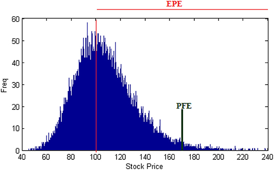
Figure 1. Undiscounted EPE and PFE for a 1 year Euro Call Option.

4. The Two Monte Carlo Methods

4.1. Steps Involved

The two simulation approaches compared here are the Least-Squares Monte Carlo [LSM-Method] [4] and Tilley Bundling [2]. In both approaches, a sample path of stock prices is first produced using the GBM method. One must be aware that the holder of an American option may exercise the option if in-the-money at predefined times up to expiry of the contract. Therefore at any of these predefined times, a decision criteria is applied as to whether the derivative should be exercised or otherwise. The option is exercised if the expected future pay-off from continuation is lower than the current payoff at any time.

The LSM-method estimates the expected payoff from continuation by a regression formula applied on all in-the-money stock price paths. The steps for pricing an American stock option using this method, assuming K times during which this option can be exercised, are summarized below. A novice may wish to consult Appendices A and B as these show the steps applied for a generation of sixteen paths.

Step 1: Determine the value of the future pay-off at time t = K for every stock price path. This would be equal to the pay-off for a European-style option.

Step 2: Determine which stock price paths are in-the-money at the previous time step (t_m). Denote the value of the pay-offs at this timestep as X and the discounted future pay-off values for these paths determined in Step 1 as Y.

Step 3: Produce a regression function in which the independent variables are X and the dependent variables are Y. Use this regression function to estimate the expected discounted future pay-off Y′ for each value of X.

Step 4: If X > Y′, the option will be exercised at time t_m. In this case the future pay-off value for these price paths is set as X, otherwise Y is maintained.

Step 5: Repeat steps 2 to 4 until t = 1.

Step 6: Determine the value of the American option as the average final discounted future pay-off.

The Tilley Bundling method sets the decision criteria by dividing the paths into a number of bundles. Assuming that N = A × B paths are simulated for K time-steps, the valuation method for an American call stock option can be summarized in the steps given below.

Step 1: Determine the value of the future pay-off at time t = K for every stock price path. This would be equal to the pay-off for a European-style option.

Step 2: Re-order the stock price paths by stock price at the previous timestep (t_m) in ascending order for a call option.

Step 3: Divide the N paths into A bundles of B paths each in the order given in step 2.

Step 4: Set the holding value of each path as the discounted mean of all future pay-off values within each bundle.

Step 5: For each path, calculate whether the present pay-off value is higher than the holding value. Set the Boolean variable X as one if this is the case or zero if otherwise. This will produce a string of ones and zeros.

Step 6: Determine one boundary that decides whether to execute the option at time t_m by finding the first string of ones whose length is bigger than each subsequent string of zeros.

Step 7: All current pay-offs higher than the boundary evaluated in step 6 would be exercised at time t_m. Record whether each path would be exercised at this time. Update the future pay-off as the current pay-off for these cases and as the holding value for all other cases.

Step 8: Repeat steps 2 to 7 until t = 1.

Step 9: Determine the value of the American Option as the mean discounted pay-off of the earlier exercise time (evaluated in step 8) for each path.

4.2. Applying the Methods to an American Put Option

4.2.1. Pricing Best-Estimate Value

The price of an American put stock option at a strike price of 40 exercisable 50 times a year was evaluated using these two Monte Carlo methods as shown in Table 1. Results based on 100,000 paths (half of which are antithetic to reduce variance) with a yearly interest rate of 6%, a number of initial stock prices ranging from 36 to 44, a volatility measure of 20 or 40%, and a one or two year time period.

TABLE 1

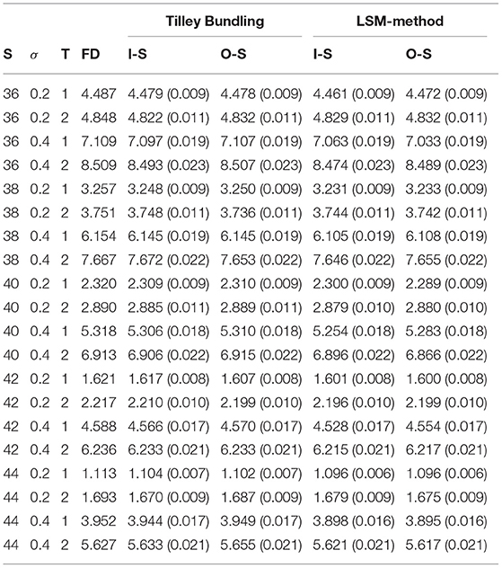
Table 1. The value of an American Put stock option. The values in brackets show standard deviation.

The Tilley bundling technique consisted of 250 bundles of 400 paths each as this value maintains a low ratio of bundles to paths as recommended in the original paper [2]. A cubic regression function was used for the LSM-method.

The price was evaluated also on an out of sample (O-S) generation for both methods. The value priced under O-S is a random generation of an additional 100,000 paths (half of which antithetic) but using the regression function as evaluated for the in sample (I-S) set under a LSM-method (step 3) or using the same boundary condition as evaluated for the I-S generation under the Tilley Bundling method (step 6).

Both methods compare favorably with the price set by the finite difference method [5] with 40,000 time steps per year over 1,000 steps for the stock price. The Tilley Bundling method is slightly superior to the LSM-method however the latter can be improved by applying more basis functions to the regression formula.

Key differences between the two methods is that conditional expectation are evaluated differently: using a global polynomial for LSM-method and constant mesh methods in the Tilley Bundling approach.

4.3. Pricing Risk

The evaluation of risk measures for an American option directly from an equation is a trickier process than for a European style option due to the early exercise features of the former. One can envisage that in this circumstance, the probability distribution function of the stock price is dependent on time and stock price [5].

This paper shows the PFE (99%) and EPE values of a one-year American put option with a strike price that is equal to the initial price of 100, a drift of 6% and volatility of 40% with 50 exercise points per year. The VaR for this contract is simply zero for all cases. Throughout this exercise, the risk measures are shown at a present value at the start of the contract.

The values of EPE and PFE are not easily obtainable from a closed-form solution to be able to make comparisons. One possible approach is to define possible minimum and maximum values. An American Option has early exercise features and hence carries more credit counterparty risk than a European style option. Therefore the minimum values could be set as the metrics for a European Option ending at the same time.

Maximum possible risk metrics can also be evaluated by taking into consideration the log-normal distribution at each of the remaining exercise points. When assuming one exercise point, the PFE is calculated as the 99th percentile. Assume that there are two exercise points (t_f, t_{f + 1}) and each are equally likely randomly exercisable. Then there exists some value such that its average percentile amount over the two distributions is 99%². This value would be considered as the maximum average PFE for these two exercise points. The PFE can therefore be found as that value that lies in the extreme 1% in-the-money value of the derivative over all remaining exercise points by solving (Equation 4). Similarly a possible maximum approximation for the EPE is finding the average expected positive exposure of all future time points (Equation 5). One can consider this as if dealing with a series of European Options each exercised at a different time point.

$\begin{array}{ll}{\Sigma }_{t=k}^{50}\left[F_2(x,t,100+PF{E}_{0.99}{e}^{0.0012t})\right]=0.01(51-k)& (4)\end{array}$

$\begin{array}{ll}EP{E}_{{\text{k}}^{\text{th}}\text{ time}}=\frac{{\Sigma }_{t=k}^{50}\left[e^{-0.0012t}{F}_2(x,t,100)(100-\frac{F_3(x,t,100)}{F_2(x,t,100)})\right]}{(51-k){\Sigma }_{t=k}^{50}{F}_2(x,t,100)}& (5)\end{array}$

where,

$\begin{array}{l}{F}_2(x,t,a)={\displaystyle {\int }_0^a\text{}}[\left({(x\sigma )}^{-1}\sqrt{\frac{25}{t\pi }}\right)\hfill \\ exp\left[-\frac{{\left(log(x)-log(S_0)-\left(\mu -\frac{{\sigma }^2}{2}\right)\frac{t}{50}\right)}^2}{{\sigma }^2\frac{t}{25}}\right]]\text{ d}x\hfill & (6)\end{array}$

and.

$\begin{array}{l}{F}_3(x,t,a)={\displaystyle {\int }_0^a\text{}}[\left({\sigma }^{-1}\sqrt{\frac{25}{t\pi }}\right)\hfill \\ exp\left[-\frac{{\left(log(x)-log(S_0)-\left(\mu -\frac{{\sigma }^2}{2}\right)\frac{t}{50}\right)}^2}{{\sigma }^2\frac{t}{25}}\right]]\text{ d}x\hfill & (7)\end{array}$

5. Results and Discussion

The EPE and PFE evaluated by the two Monte Carlo methods are more straightforward. These are calculated as the mean of all positive values and the ninety-ninth percentile of the expected future pay offs calculated at steps 4 (LSM-method) and 7 (Tilley Bundling). One hundred thousand simulations are used to compare our results as shown in Figure 2.

FIGURE 2

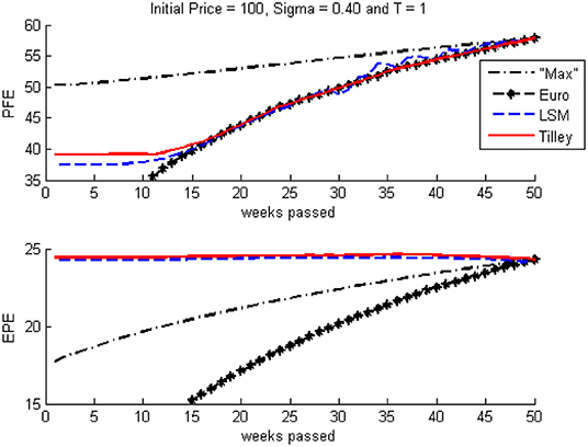
Figure 2. EPE and PFE for an American Call Option simulated using Tilley Bundling and LSM.

In every simulated scenario, a number of observations can be made. Firstly all metrics are larger than the European style equivalent which is a trivial result. However any estimate is closer to the European style option when nearing the end of the option since the American style option would have a lower number of exercise points. LSM produces less stable results since this is dependent on the regression formula produced.

The estimated maximum PFE is significantly larger than the valuation from the two methods since, in cases of an option being in-the-money by a large present pay-off value, it is very likely that this is exercised early and therefore reducing the likelihoods of later even higher in-the-money pay-off values. The maximum EPE is lower for a similar reason. At the start of the contract, a contract with a low value would not be exercised as it would have a higher expected future value than the current value.

In order words, the early exercise feature diminishes the likelihoods of either very extremely high or very low pay-off values when compared to cases where the option is exercised at a random time step as the direct method (Equations 4 and 5) indicates. Consequently the features of the contract diminish the positive skewness of outcomes, hence increasing the mean and reducing large percentile values. This justifies the results of EPE and PFE respectively of the two valuation methods when compared to the limits set in Equations (4) and (5).

The two methods described here have been under scrutiny for twenty years but most published applications focus on pricing the value of a derivative rather than the attached risk. This is accentuated by the fact that risk measures have been under the spotlight in greater detail only after the 2008 crisis. The LSM-method has resulted in oscillations in regressions especially when adding more dimensions of the basis. Bouchard and Warin [11] recommend different approaches to avoid oscillations. Nonetheless the aim of this work has been to show that techniques that are known to estimate the best-estimate correctly may differ in risk pricing, even under simple assumptions.

It would be of interest to investigate how these models act under a full economic cycle. Moreover, future work should investigate more hybrid methods such as applying piecewise regression (as in essence Tilley Bundling is a piecewise regression with the regression function being a constant), logistic regression applied to both methods, and multi-dimensional sorting under a Tilley bundling scheme (such as KNN) for more exotic derivatives.

Author Contributions

The author confirms being the sole contributor of this work and has approved it for publication.

Conflict of Interest

The author declares that the research was conducted in the absence of any commercial or financial relationships that could be construed as a potential conflict of interest.

Acknowledgments

This work has appeared in the author's Ph.D dissertation [12] and an earlier version presented at the 2013 Actuarial Research Conference hosted by Temple University [13] where it won best presentation award. The author thanks earlier commentators of this work. The author is thankful for the endless discussions with Juxo Li and Rickard Branvall.

Supplementary Material

The Supplementary Material for this article can be found online at: https://www.frontiersin.org/articles/10.3389/fams.2019.00060/full#supplementary-material

Abbreviations

EPE, Expected Positive Exposure; FD, Finite Differences; GBM, Geometric Brownian Motion; I-S, In-Sample; KNN, K-nearest-networks; LSM-method, Least Squares Monte Carlo method; O-S, Out-of-sample; PFE, Potential Future Exposure; S, Initial stock price; σ, volatility.

Footnotes

1. ^It is possible that a VaR is a value that is in-the-money in the case of a derivative that has high likelihood of being profitable. Alternatively the VaR could be the premium paid. In this paper, any premium paid is considered a sunk cost and hence not included in the risk metrics.

2. ^For example this value might be the 98.5th percentile at t_f+1 and the 99.5th percentile at t_f.

References

1. Hull JC. Options, Futures and Other Derivatives, 2nd ed. Boston: Prentice Hall (1993).

Google Scholar

2. Tilley JA. Valuing American options in a path simulation model. Trans Soc Actuar. (1993) 45:104.

Google Scholar

3. Fu MC, Laprise SB, Madan DB, Su Y, Wu R. Pricing American options: a comparison of Monte Carlo simulation approaches. J Comput Finance. (2001) 4:39–88. doi: 10.21314/JCF.2001.066

CrossRef Full Text | Google Scholar

4. Longstaff FA, Schwartz ES. Valuing American options by simulation: a simple least-squares approach. Rev Financ Stud. (2001) 14:113–47. doi: 10.1093/rfs/14.1.113

CrossRef Full Text | Google Scholar

5. Hull JC. Options, Futures and Other Derivatives, 8th ed. Boston: Prentice Hall (2012).

Google Scholar

6. Boyle PP, Broadie M, Glasserman P. Monte Carlo methods for security pricing. J Econ Dynam Control. (1997) 21:1267–321.

Google Scholar

7. Barbara C, Cortis D, Perotti R, Sammut C, Vella A. The european insurance industry: a PEST analysis. Int J Finan Stud. (2017) 5:14. doi: 10.3390/ijfs5020014

CrossRef Full Text | Google Scholar

8. Linsmeier TJ, Pearson ND. Risk Measurement: An Introduction to Value at Risk. EconWPA (1996). Available online at: http://ideas.repec.org/p/wpa/wuwpfi/9609004.html.

Google Scholar

9. Gregory J. Counterparty Credit Risk: The New Challenge for Global Financial Markets. Chichester: The Wiley Finance Series. John Wiley & Sons (2010). Available online at: http://books.google.com.mt/books?id=WZ_vbGGx1z4C.

Google Scholar

10. Glasserman P. Monte Carlo Methods in Financial Engineering (Stochastic Modelling and Applied Probability), 1st ed. New York, NY: Springer (2003). Available online at: http://www.amazon.com/exec/obidos/redirect?tag=citeulike07-20&path=ASIN/0387004513

Google Scholar

11. Bouchard B, Warin X. Monte-Carlo valuation of American options: facts and new algorithms to improve existing methods. In: Carmona RA, Moral PD, Hu P, Oudjane N, editors. Numerical Methods in Finance. Berlin: Springer Berlin Heidelberg. (2012). p. 215–55.

Google Scholar

12. Cortis D. Betting Markets: Defining Odds Restrictions, Exploring Market Inefficiencies and Measuring Bookmaker Solvency. (2016). Available online at: https://lra.le.ac.uk/handle/2381/37783

Google Scholar

13. Branvall R, Cortis D, Li J. Pricing risk through simulation: revisiting Tilley bundling and least squares Monte Carlo methods. In: The 2013 Actuarial Research Conference. (2013).