 Roland Potthast
 Christian A. Welzbacher
94% of researchers rate our articles as excellent or good
Learn more about the work of our research integrity team to safeguard the quality of each article we publish.
Find out more
ORIGINAL RESEARCH article
Front. Appl. Math. Stat., 23 October 2018
Sec. Dynamical Systems
Volume 4 - 2018 | https://doi.org/10.3389/fams.2018.00045
This article is part of the Research TopicData Assimilation and Control: Theory and Applications in Life SciencesView all 10 articles
The goal of this work is to analyse and study an ultra-rapid data assimilation (URDA) method for adapting a given ensemble forecast for some particular variable of a dynamical system to given observation data which become available after the standard data assimilation and forecasting steps. Initial ideas have been suggested and tested by Etherthon 2006 and Madaus and Hakim 2015 in the framework of numerical weather prediction. The methods are, however, much more universally applicable to general non-linear dynamical systems as they arise in neuroscience, biology and medicine as well as numerical weather prediction. Here we provide a full analysis in the linear case, we formulate and analyse an ultra-rapid ensemble smoother and test the ideas on the Lorentz 63 dynamical system. In particular, we study the assimilation and preemptive forecasting step of an ultra-rapid data assimilation in comparison to a full ensemble data assimilation step as calculated by an ensemble Kalman square root filter. We show that for linear systems and observation operators, the ultra-rapid assimilation and forecasting is equivalent to a full ensemble Kalman filter step. For non-linear systems this is no longer the case. However, we show that we obtain good results even when rather strong nonlinearities are part of the time interval [t0, tn] under consideration. Then, an ultra-rapid ensemble Kalman smoother is formulated and numerically tested. We show that when the numerical model under consideration is different from the true model, used to generate the nature run and observations, errors in the correlations will also lead to errors in the smoother analysis. The numerical study is based on the popular Lorenz 1963 model system used in geophysics and life sciences. We investigate both the situation where the full system forecast is calculated and the situation important to practical applications where we study reduced data, when only one or two variables are known to the URDA scheme.
Data assimilation is concerned with the use of observation data to control or determine the state of some dynamical system [1–3]. Data assimilation methods are indispensable ingredients to calculate forecasts of some system, with universal applicability ranging from neuroscience [4, 5] to weather forecasting [6–8], from systems engineering like traffic flow [9–11] to geophysical applications [12, 13].
Over time several generations of data assimilation methods have been developed, for example optimal interpolation in the 70th, variational methods in the 80 and 90th and ensemble data assimilation since about 1995, with very intense research activities since about 2000 (e.g., [1–3, 14]). Today, ensemble data assimilation methods for example for numerical weather prediction are run daily on modern supercomputers by operational centers such as Deutscher Wetterdienst (DWD, Germany), European Center for Medium Range Weather Forecast (ECMWF, Reading, UK), or the MetOffice in the UK.
Usually, data assimilation takes observations y and combines them with first guess model states x(b) (also called the background) to estimate a best possible analysis x(a). Usually, the estimation of the analysis state is performed in turns with short-range forecasting, i.e., within a given temporal framework assimilations are carried out at times tk for k = 1, 2, 3, …. Short range forecasts calculate the state by applying the model dynamics M to the initial state given by the analysis at time tk−1. Then, the core analysis step is carried out at time tk, based on observations which are available either at tk or in the interval [tk−1, tk]. Alternating short-range forecasts and core analysis steps leads to the classical data assimilation cycle. Often, forecasts are then calculated based on selected analysis states and analysis times.
Today, many forecasting systems have moved away from pure deterministic forecasting and employ ensemble prediction systems (EPS), where several forecasts with different initial conditions (and sometimes different physical or stochastical parameters) are calculated. Based on an ensemble of states, the uncertainty of the forecast can be estimated. Further, the ensemble allows to determine dynamical spatial and temporal correlations, which help to improve the analysis itself and can serve as input for probabilistic diagnostics.
Often, for large-scale realistic systems, the model forecast as well as the analysis step needs huge computational resources. They limit the temporal resolution of the data assimilation cycle. Further restrictions are given by the availability of observations, which need to be measured and distributed to reach operational centers. For example, to run an assimilation cycle of 1 h for convection permitting high-resolution numerical weather models, top-500 supercomputers are needed to achieve a sufficient resolution and spatial extension of the model fields under consideration [8].
The core task addressed in this work is the problem of ultra-rapid data assimilation (URDA), in the case where standard data assimilation cycles have clear limits with respect to speed and flexibility. We assume that a classical data assimilation cycle is available, such that we can calculate an ensemble of forecasts for some time interval [t0, tN]. The next classical analysis is calculated for time tN, such that a similar ensemble forecast will be available for a subsequent interval [tN, tN+1]. Here, we limit our interest in the ultra-rapid data assimilation for observations yk which are available at points in time tk with t0 < t1 < t2 < … ≤ tN. The task is to provide an update of the ensemble forecast with high speed without using the full numerical model or a full-grown data assimilation system. In particular when we are interested only in the forecast of some layer or part of the state space, this is of high practical interest.
Usually, the classical forecast cycle in operational centers is based on a data assimilation cycle with frequency tN of several hours. The term rapid update cycle (RUC) is used when cycling and forecasting is carried out hourly or subhourly. The term ultra-rapid update cycle is used when we go to a cycling interval which is much smaller, e.g., 5 min. Further, to achieve this speed we cannot initialize the full model in each step. The approach of ultra-rapid data assimilation—though embedded into a RUC or classical cycle—does not use the classical setup of cycling model and assimilation step any more for its updates. Further, it works with a subset of model variables only. The speed-up is achieved by the conceptional changes within the full cycle, not alone within the data assimilation step itself.
We will base ultra-rapid data assimilation on the ensemble transformation matrix given by the ensemble Kalman filter (EnKF) or ensemble Kalman square root filter (SRF), compare [15–19]. The basic idea of ultra-rapid data assimilation is to employ a reduced version of the state variables which are made available to the system. Measurements of some of these variables can be employed to calculate an ensemble Kalman transformation matrix1. This Matrix is used to update both the analysis ensemble as well as the forecast ensemble. For linear model systems and linear observation operators, we will see that the forecasts based on the analysis ensemble and the transformed forecast ensemble are identical. This is true both for the full analysis and forecasting as well as for the case where we base our analysis and forecasting transformation on a reduced set of model variables or diagnostic ensemble output.
To study the quality of ultra-rapid data assimilation we apply the basic ideas to the Lorenz 1963 model [[20], see also for example [21–24] and [3] Chapter 6]. Here, we generate some truth by running the model with a particular setup. Observations are simulated and drawn with random perturbations. Then, a model with a different setup is used to assimilate the observations either with the ultra-rapid assimilation scheme and for comparison by running a full ensemble Kalman filter for each of the time-steps tk, k = 1, …, N. We study the case of reduced variables and provide diagnostic results for the ensemble Kalman smoother over the full time interval [t0, tN].
The approach discussed here was first suggested in the work of Etherton [25], where the term preemptive forecast was coined and the method was tested for a barotropic model. The ideas have been picked up by Madaus and Hakim [26], where the authors applied the approach to ensemble forecasts of numerical weather models, obtaining a so-called ensemble forecast adjustment. In the latter work the advantage of the method, that rapid updates of (subspaces of) model predictions without rerunning a full dynamical model again, are highlighted. They focused on global scales and corresponding time scales and observables for a particular application. Here, we provide additional contributions to the mathematical analysis for linear systems. Further, we formulate and investigate the ultra-rapid ensemble smoother and extensively study the non-linear Lorentz 63 system, which serves as a very popular reference system for geophysics and life sciences.
In section 2 we introduce our notation and basic results from ensemble data assimilation. In particular, we introduce the ensemble Kalman filter in the notation of Hunt et al. [16] and Nakamura and Potthast [3]. We also discuss the role of reduced variables for the ensemble Kalman square root filter. Section 3 serves to introduce and investigate details of the ultra-rapid data assimilation, with the data assimilation analysis and forecasting in section 3.1 and the ultra-rapid ensemble smoother in section 3.2. Numerical examples are shown in section 4, with generic results on the assimilation and forecasting in section 4.1 and the study of reduced variables in section 4.2. Conclusions are given in section 5.
This section serves to collect notation and basic results on the ensemble Kalman square root filter (SRF) following the notation of Hunt et al. [16] and Nakamura and Potthast [3]. The SRF is our reference for full-scale forecasting and it provides the core ingredients of our ultra-rapid data assimilation algorithms as described in section 3.
We consider a state space ℝn, an observation space ℝm with n, m ∈ ℕ, states x ∈ ℝn and observations y ∈ ℝm. The basic idea of the ensemble Kalman filter type methods such as the SRF is to approximate the covariance matrix B ∈ ℝn×n of the system based on some ensemble xb, (ℓ), ℓ = 1, …, L of L ∈ ℕ states in the form
where
is the matrix Qb ∈ ℝn×L of centered differences (sometimes its columns are called the centered ensemble) with the ensemble mean
Note, by construction the space spanned by the member of the centered ensemble has dimension L − 1 and one can define the full ensemble matrix
In order to assimilate observation data the model equivalents yb, (ℓ) of the ensemble member are required, which are obtained by applying the observation operator H:ℝn → ℝm to the corresponding ensemble member
With these quantities the matrix Tb ∈ ℝm×L can be defined analogously to Qb
which one also denotes as Tb = HQb assuming a linear operator H.
In the following, + between a vector and a matrix indicates a column-wise summation a + A = (a + a1, …, a + aL) with the columns a ℓ , ℓ = 1, …, L of the matrix A, such that we can add column vectors and matrices in one joint notation. The generic update equation for an ensemble type data assimilation can be written in different forms, in particular
with the transformation matrices computed in ensemble space and , depending on the vectors and matrices and the observation error correlation matrix R∈ℝm×m. We quickly review the different versions as follows. An analysis update of the centered ensemble (see Equation 4) given by
leading to Equation(8). In Equation (9) we have used an update of the ensemble mean
with , which is naturally defined by the Ensemble Kalman Filter – details will be given below. Equation (10) just collects the increment in terms of Qb. The definition of the transformation matrix
leads to the update Equation (11). For the full transform matrix Wfull we obtain
based on
and by
Different notations have been used over time, depending on whether you want to keep your equations close to the classical Kalman filter equations or for a more practical focus. The quantities defined in Equations (2, 6) differ from the definitions of Xb and Yb of Hunt et al., c.f. Equations (12, 18), by the normalization factors. The relations are
The full ensemble matrix has different letters , we also note the identity Wa = S between Hunt et al.[16] and Nakamura and Potthast[3]. Some equations are modified. For example Equation (4) changes to
the update of the mean Equation (14) rewrites as
with and Equations (8, 10) are written as
The transformation matrix in the sense of Equation (25), giving us the increment in ensemble space, is now given by
The ensemble Kalman filter combines the above introduced notion of an ensemble of model states to describe spatial and temporal correlations with the well-known Kalman Filter [27]. The pending task of generating an analysis ensemble obeying an obtained analysis correlation matrix can be completed by a square root filter (SRF), originating from the Kalman filter update for the correlation matrix applied to the ensemble representation
with the Kalman gain matrix
and the transformation matrix S given by
Taking the square root of the symmetric matrix U results in
which is the transformation matrix of the update for the centered ensemble in Equation (8). Note, the notation in Equations (2, 6) is the one used by Nakamura and Potthast [3] and differs from the one introduced by Hunt et al. [16] (see Equation 19). However, by multiplying S in Equation (30) with the inverse of Wa defined by Hunt et al, the identity Wa = S can be easily shown.
The update of the mean is obtained along the lines of the classical Kalman filter by
with K given in Equation (28). Comparing Equation (14, 31) leads to
in case of the SRF. The update for the full ensemble using the ensemble Kalman square root filter is therefore given by applying Equations (30, 31) to Equation (11, 15).
Here, we can now confirm the validity of Equation (17). From the definition of Qb we know that the sum of the rows of Q is zero, such that the sum of the column of with any matrix A ∈ ℝn×L is zero, and the sum of the columns of I − (Qb)TA is one. If I − (Qb)T A is symmetric, this means that the vector equal to 1 in each component is an eigenvector of I − (Qb)T A with eigenvalue 1. But then it will also be an eigenvector with eigenvalue 1 for each power of I − (Qb)TA, such that (17) is satisfied.
Before we investigate ultra-rapid data assimilation based on reduced data, we need to recall how a standard ensemble Kalman square root filter will react when we base our analysis on a reduced set of model variables. Let us study the calculation of the ensemble analysis for the ensemble Kalman filter with reduced data. The basic formula for the ensemble Kalman filter can be expressed as with S and given in Equations (30, 32)
Now, assume we observe y ∈ ℝm which depends on some subset x1, …, xñ of the full set of variables x1, …, xn only. Given these reduced spaces the operator H will be of the form
In this case, the terms HQb ∈ ℝm×L and (HQb)T ∈ ℝL×m will be a linear combination of the variables 1, …, ñ of the ensemble members. If we are given the variables x1, …, xñ of the ensemble members only, the matrix W will not change. Also, y − Hxb will depend only on the variables of xb. The solution z ∈ ℝm of
is calculated based on the variables x1, …, xñ of Qb and of xb only. We summarize the result of these arguments in the following lemma.
LEMMA 2.1. If we have observations y dependent only on the variables x1, …, xñ for ñ ∈ {1, …, n} of the full state x ∈ ℝn of the state space of our dynamical system, the transformation matrix W of the ensemble Kalman square root filter update xa − xb depends on these variables of the centered ensemble Q and the mean first guess only.
A consequence of the above Lemma 0.0.1 is that, if we have reduced observations, the ensemble Kalman square root filter will give us an update matrix W which depends only on the variables under consideration.
But we need to pay attention to the update and propagation step. The update Equation (11) clearly updates all variables, since W ∈ ℝL×L, and thus all variables of x are updated by the ensemble Kalman filter. If the model M is based on all variables, in general we expect model propagation to be dependent on all variables as well. In general, an update based on the transformation matrix W will change all variables of the initial state. This means that the first guess of the next assimilation step highly depends on the application of the matrix W to all variables, not only to the variables x1, …, xñ.
Clearly, in general we cannot run the full ensemble Kalman filter on a reduced set of variables, just because you need all prognostic variables to run the numerical model. We will see later, that this limitation does no longer apply when we are in the framework of ultra-rapid data assimilation.
This section serves to develop the main ideas of ultra-rapid analysis, forecasting and smoothing. We will first describe the idea of ultra-rapid analysis when observations yk are given at point of time tk, k = 1, …, N throughout a time interval [t0, tN] for which we are not able to employ a full data assimilation functionality. We assume that we have been able to perform some ensemble data assimilation scheme prior to the time t1 at time t0 and that a forecast ensemble has been calculated, such that
is available at the points in time tξ, ξ = 0, …, N and for the ensemble index ℓ ∈ {1, …, L}. Note that corresponds to the analysis of the full ensemble data assimilation. We are now successively at times t1, t2, …receive observations y1, y2, … The goal is to provide ultra-rapid updates for estimation of our state at times t1, t2, … When we are at time tk, we would like to update the forecasts at the times tξ for ξ = k, …, N and obtain the best possible estimate in an ultra-rapid forecasting step.
Note, the assimilation of observations at some point in time exhibits information about the past as well. This is called smoothing. We will describe an ultra-rapid ensemble smoother in a second step. We focus on the analysis and forecasting in section 3.1 and discuss smoothing in section 3.2.
Assume that we are given some ensemble of L states of our dynamical system at time tk ∈ ℝ, which could be an analysis or a first guess from somewhere. Further, we assume that we have applied our model M to calculate forecasts based on at times tk+1, …, tN for N > k. The corresponding forecasts are denoted by for ξ = k + 1, …, N, analogous to (35).
We employ the following matrix notation. The matrix F is the matrix of the full forecast ensemble members in its columns, i.e.,
of forecasts from tk to tξ. The matrix W(k) is the matrix of linear ensemble transform coefficients calculated based on the observations yk at time tk and the first guess ensemble at time tk, i.e.,
When the analysis ensemble at time tk is given by a generic ensemble data assimilation approach, we know that
with the matrix , j, ℓ = 1, …, L given by Equation (16) with the two quantities and S being dictated by the specific ensemble data assimilation system (e.g., Equations 30, 32), where the time index k refers to the analysis time tk for which Wj, ℓ is calculated. Also, we note that the background is given by
LEMMA 3.1. Here, we assume that the model M is a linear model M. In this case, the forecast ensemble at time tξ when observations at time k are assimilated by a linear data assimilation method as in Equation (12), the forecast ensemble can be calculated by
Proof. In this case we have
for ℓ = 1, …, L and ξ ∈ {1, …, N}, where we used Mk − 1, ξ = Mk, ξMk − 1, k. □
Before we continue with our introduction of ultra-rapid data assimilation, we would like to study the reduced variable case in the above Lemma 0.0.2. Clearly, to apply Mk, ξ to a state x(a) or x(b), we need to know the full state. If only a part of the state x is available, starting the model is no longer possible. However, the Equation (40) is still valid for each of its components, i.e., if W is known, the variable of can be calculated from the knowledge of for all ℓ = 1, …, L, representing the i-th variable of the state vector of the l-th ensemble member obtained by a forecast from time tk − 1 to time tξ.
COROLLARY 3.2 (REDUCED SET OF MODEL VARIABLES). If the observation operator H depends on the variables x1, …, xñ of the state x only, then the transformation matrix W(k) for the assimilation of yk can be calculated from a) the first guess ensemble data and b) the observation yk. For a linear model M, for the variables with index i we have
for i = 1, …, ñ, i.e., the formula (40) is valid and the ensemble forecast based on the analysis with observation yk can be calculated from the knowledge of the reduced set of variables only.
The consequence of Equation (41) is that for linear models we can calculate the forecast based on the analysis at time tk by a superposition of the forecast from time tk − 1. The weight matrix is calculated from the ensemble analysis at time tk given by the linear ensemble data assimilation scheme. We can also use Equation (41) recursively, which is formulated in the following Theorem.
THEOREM 3.3. We assume we are given observations yj, j = 1, …, k at times t1, …, tk. The goal is to calculate the forecasts at time tξ based on the observations from t1 to tk and the initial ensemble at time t0 with an ensemble data assimilation method as in Equation (11). If the model M is linear, we obtain
for ξ = k+1, …, N.
Proof. For a linear model, the generic step is given by Equation (41). Then, the same equation is applied to , which leads to
and by the same step η times to
for η ≤ k assimilation steps. In matrix notation and for η = k this is Equation (43). □
Note that the recursive application of Equation (41) implies that any transformation matrix W(i) is obtained using the observation yi and the full ensemble Fi − 1, ξ.
The results for reduced data are also valid for the core formula (43). We collect the relevant statements into the following corollary. The matrix Fk, ξ contains the different state variables in its rows and the columns represent the ensemble under consideration. We employ the notation (Fk, ξ)i = 1, …, ñ for the rows with the variable indices i = 1, …, ñ.
COROLLARY 3.4 (REDUCED Set of MODEL VARIABLES). If the observation operator H depends on the variables x1, …, xñ of the state x only, then the transformation matrix W(k) for the assimilation of yk can be calculated from a) the first guess ensemble data (F0, k)i = 1, …, ñ, b) the observation yk and c) the previous transformation matrices W(1)⋯W(k − 1) which depend on the corresponding observations y1⋯yk − 1. For a linear model M, for the variables with index i we have
i.e., the formula (43) is valid and the ensemble forecast based on the analysis with observation yk can be calculated from the knowledge of the reduced set of variables only.
Smoothers are schemes which employ information from the future to improve the estimate about some present state. Alternatively, you could say that they use information now to update past states.
When we consider the scenario of ultra-rapid data assimilation, for the interval [t0, tN] we are given an ensemble of original states (35) over the full interval. When an observation is arriving at time tk (ignoring delay usually needed for observation processing and transfer), we can employ the same techniques which are used for updating the analysis and forecast to the past interval [t0, tk].
DEFINITION 3.5 (ULTRA-RAPID ENSEMBLE SMOOTHER).
Given the original first guess ensemble F0, ξ for ξ = 0, …, N on the time interval [t0, tN] we define the ensemble analysis given the data y1, …, yk by
This analysis ensemble is defined for the full time interval.
In general, a convergence analysis of an ensemble Kalman smoother and its comparison to a four-dimensional variational data assimilation (4D-VAR) scheme over the time window [t0, tn] can be found in Theorem 5.4.7 of Nakamura and Potthast [3]. For linear models and observation operators, the full Kalman smoother and 4D-VAR are equivalent.
Clearly, if we replace the full model M by the ensemble, this equivalence is no longer true. Also, if the numerical model M used to calculate the ensemble is different from the true model Mtrue, the temporal correlations, which are implicitly used when we employ the analysis matrix W(k) to update the ensemble in the past or in the future, may not be correct with respect to the true ensemble correlations. In this case, the information yk in the future of t0 may not improve the state estimate at time t0, but lead to additional errors in this state estimate. We will demonstrate this phenomenon in our numerical examples in section 4.
The goal of this section is to study the ultra rapid data assimilation for simple generic examples. We want to show that the assimilation step can be carried out in a stable way and that the ultra-rapid forecasts indeed show an advantage over the ensemble forecasts without this step. Also, we would like to understand the range of skill which we can achieve when we compare it with the full standard data assimilation and forecasting approaches.
Here, we start our study with the Lorenz 63 model Lorenz [20]. It is a very well-known chaotic ODE system with three unknowns, compare for example Nakamura and Potthast [3].
The Lorenz 1963 model is a system of three non-linear ordinary differential equations
with constants σ, ρ, β known as Prandtl number, the Rayleigh number and a non-dimensional wave number. Here, for the constants we take the classical values σ = 10, β = 8/3 and ρ = 28. The implementation of the system is usually carried out by a higher-order integration scheme such as 4th-order Runge-Kutta, which we have employed for our numerical testing. The setup for our case study is shown in Figure 1A with 8 cycles for better visibility and Figure 1B with 40 cycles for studying the error evolution.
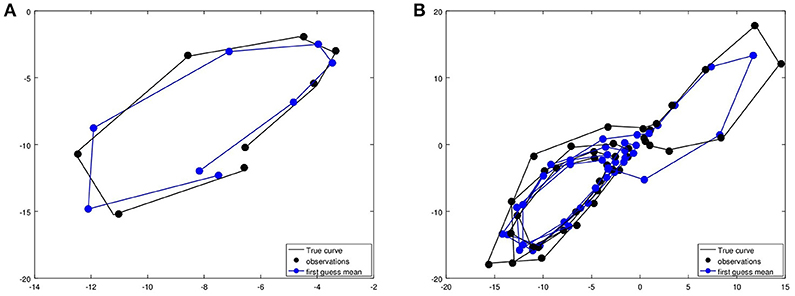
Figure 1. We show the simulation of some trajectory by the Lorenz model in black, the first 8 cycles in (A), then 40 cycles in (B). The observations, which are calculated by adding some Gaussian random error to the true observations, are shown as black dots. Here, we assume that we observe all three variables of the model. The first guess trajectory as a blue curve. The first guess states for the observation time steps are shown as blue dots.
Here, we want to test the feasibility of ultra rapid data assimilation. The original curve is shown in black in Figure 1. The measurements are calculated by adding a random Gaussian error to this curve at the measurement times t1, t2, …, tk with Δt = ti+1 − ti = 0.1 (without units). For the original, we have used the above ODE system with σ = 10 to generate the truth. To test data assimilation we have employed a modified system where σ = 12 was chosen. The mean of the original first guess ensemble for the full time period under consideration is shown in Figure 1 as a blue curve, with blue dots as the original first guess.
We have now followed two tracks. First, we have implemented an ensemble Kalman square root filter. We start with a first guess ensemble, which is generated at time t0 by adding random Gaussian errors to the starting point of the original curve. Then we assimilate the observations (the black dots) using the Ensemble Kalman square root filter.
Second, the ultra-rapid data assimilation and forecasting cycle has been implemented. The ultra rapid data assimilation has been set up by first calculating the full first guess ensemble for the whole time interval under consideration. Then, a modified ensemble is calculated step by step following (43). We study N time steps (showing results for N = 8 and N = 40). In more detail, we have calculated the transformation matrix W(k) based on the observations yk at time tk, k = 1, …, N and the transformed first guess ensemble . Here, ξ is the time index of the ensemble, i.e., ξ = 1, …, N. We carry out the assimilation for all time steps, changing the ensemble in the past as well as in the full future over the time interval under consideration.
The result of N time steps is shown in Figure 2. First, the example with N = 8 time steps is shown in Figure 2A,B, the first guess errors for N = 25 and N = 40 time steps in Figure 2C,D. Here, initially the ultra-rapid update is quite good, approximating well the full ensemble Kalman square root filter over 10 or 15 assimilation steps. Then, when the first guess ensemble and the true trajectory diverge further, the assimilation looses track and we obtain very large errors over time, as can be seen by the peak of the pink curve in Figure 2D at about tk with k = 34.
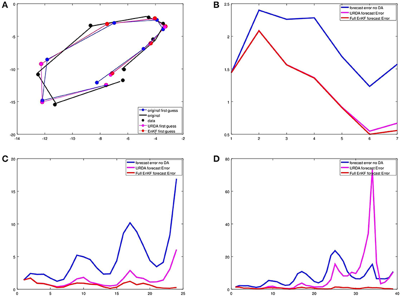
Figure 2. We show the results of the ultra rapid data assimilation in comparison with the ensemble Kalman square root filter for the Lorenz 1963 model for N = 8 assimilation steps. In (A), the black curve is the original, black dots are the observations. The mean of the analysis ensemble of the ultra rapid data assimilation URDA after k = 8 assimilation steps is shown in pink, where we need to note that here the information of the data is used to update the full curve at all points (i.e., the estimate of the past is updated as well. The red curve shows the analysis ensemble mean of the sequential ensemble Kalman square root filter. (B–D) show the sequential error curves of the analysis error, pink for URDA, red for the ensemble Kalman square root filter.
Here, we also investigate the ultra rapid data assimilation tool as a smoother. We calculate the analysis ensemble defined in (47) based on the original first guess ensemble F0.
In Figure 3 we study the filter and smoother results for a case with N = 32. For the latter we update both the future and the past. Errors of this with respect to the true curve are displayed in Figure 3C,D. Here, we need to note that we simulate a realistic setup in the sense that the true model Mtrue is different from the model M used to calculate the first guess ensemble. That has severe consequences for the convergence of the smoother. With the errors in the model, we obtain errors in the first guess ensemble and with this errors in the correlations and covariances which are exploited by the ultra-rapid Kalman filter forecast and the update of the past in the ensemble Kalman smoother.
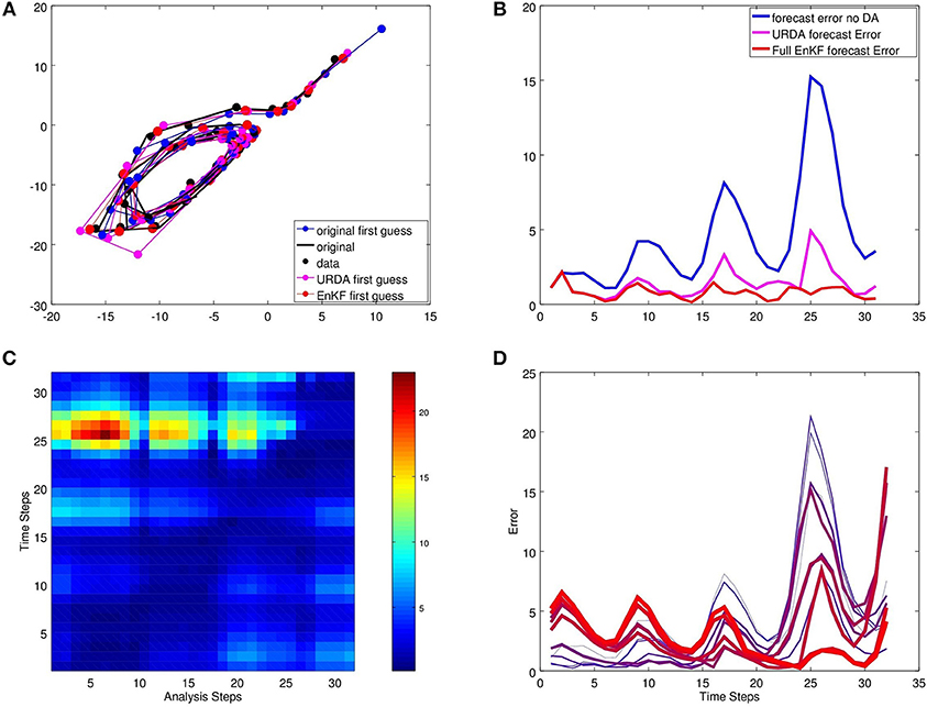
Figure 3. Studying the results of the ultra-rapid ensemble smoother over N = 32 assimilation steps. (A) shows the original data and the first guess of the Kalman filter analysis cycle. The corresponding first guess error is compared in (B). (C,D) show the error of the full ultra-rapid ensemble analysis for the full time-scale between t0 and tN for N = 32 time steps. In (D) we display the error for the curves t1, t4, t7, …, t31, starting with a thin blue curve and ending with a thick red curve.
Studying Figure 3C we see that the error is smallest on the diagonal, i.e., for the analysis and short-term forecast based on the ultra-rapid ensemble Kalman analysis. The errors for the analysis or forecast increase with distance to the current point in time. We expect that the errors are large for larger lead times. But in general we do not expect that the errors in the past, i.e., at the beginning of the interval [t0, tN] increase when we assimilate more and more data. When the ensemble reflects the correct correlations between the future and the past, the error should decrease. However, with a numerical model which is different from the true model, we also inherit errors into the temporal correlations. As a consequence we observe that the error at t1 increases when we assimilate further data yk for k in the second part of the interval [t0, tN].
In Figure 4 we evaluate the performance of URDA in a statistical manner by using different initialisations for the applied random number generator, which affects the observations drawn from a Gaussian distribution as well as the construction of the ensemble, and use different values of the starting point x0 = x(t0), which is used to obtain the truth as well as the ensemble. We evaluate differences of the corresponding mean from the truth and take appropriate ratios. In Figure 4A the mean-error of URDA is divided by the mean error of the free forecast (no data assimilation, also abbreviated by no-DA) for L = 5 ensemble member and N = 25 time steps on the trajectory. A clear positive impact is visible with only very few cases where the free forecast is better than URDA. Figure 4B shows the mean-error of the SRF divided by the one of URDA. As expected, the evaluation shows that in many cases the full SRF performs better compared to URDA. However, comparing with the results shown in Figure 3C this is what we expect due to the deviations after about N = 8 time steps. To test this, we show the result for the first 8 time steps of the run with N = 8 in Figure 4C and observe, that for a smaller N these compete indeed much better with the SRF. Figure 4D shows the result of the mean-error of URDA divided by the initial forecast with no data assimilation for L = 25 ensemble member and N = 25 time steps. We observe, that the improvement of URDA with L = 25 compared to L = 5 is not significant. This is no surprise since we deal with three prognostic variables where an ensemble of L = 5 is already sufficient to describe the relevant spread.
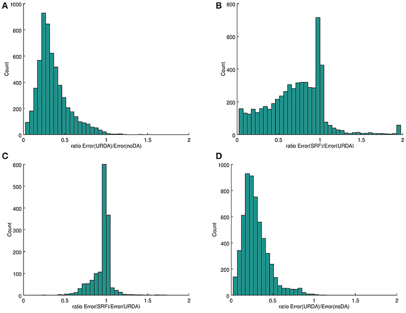
Figure 4. We show the results of the mean-error of the ultra rapid data assimilation in comparison with the original first guess (no data assimilated) and the ensemble Kalman square root filter for the Lorenz 1963 model. We used Nstat = 250 different initializations of the random number generator to obtain different distributions for the observations and the initial ensemble. After assimilation of all data the mean error at each time step on the trajectory from the truth is counted. In (A,B) we used L = 5 and N = 25 to obtain histograms showing in (A) the ratio of the mean-error of URDA divided by the mean-error of the model forecast without data assimilation. For L = 5 in (B) the mean-error of the SRF divided by the one of URDA is displayed for N = 25 while the same is shown for N = 8 in (C). The ratio of the mean-error of URDA divided by the initial forecast for N = 25 and L = 25 in (D).
At the end of this section we highlight the impact of the time step in the model, which translates to the time the forecast from one point on the trajectory is performed. Note, this does not affect the performance of the Runge-Kutta-Scheme where the time step of the integration is kept fixed. We evaluate the ratio of the deviations from the mean error from the SRF to URDA. In Figure 5 we show results for different sizes of the time step dt. Again we used Nstat = 250 and the total number of time steps N = 25 with the number of ensemble members L = 5. We observe, that for 1/4 of the standard time step size dt = 0.100 the SRF and URDA perform almost equally. With increasing time step size we find more cases where the SRF outperforms URDA, which is still moderate for the standard time step size. For three times this step size we see a clear benefit for the SRF. Note, since we keep N = 25 fixed, the total length of the trajectory differs for the different time step sizes dt.
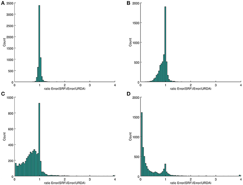
Figure 5. We show the ratio of the mean-error of the SRF divided by the one of URDA for different step sizes in time. Specifically, in (A) we used dt = 0.025, in (B) dt = 0.050, in (C) the standard value dt = 0.100 and in (D) dt = 0.300.
In the second part of our numerical study we would like to understand how ultra-rapid ensemble data assimilation can be applied to the case where only a reduced set of variables is passed down from the standard ensemble data assimilation framework.
In the framework of the Lorenz model, we have carried out a study the use of the observation operators
and study assimilation of observations of either the full state x, the first two variables of the state or the first variable of the state only.
We note that HQ will employ the corresponding selection of variables depending on the cases H1, H2 or H3, i.e., H1Q can be calculated from the knowledge of the first variable x1 of only. Similarly, H2Q can be calculated based on the knowledge of (x1, x2) of .
Here, we focus on the results for the use of H2 in Figure 6. The effects are similar to the three-dimensional version. Figure 6A displays the first 8 steps, and we see that the SRF analysis and the URDA analysis are very close to each other. The error is shown in Figure 6B, here only for the two variables under consideration. Figure 6C,D display 30 assimilation setups. After 20 and 25 steps we observe first cases where URDA is worse than no-DA. In all other cases it is a big increase from the no-DA case and its quality becomes close to the quality of the full square-root filter with subsequent forecast.
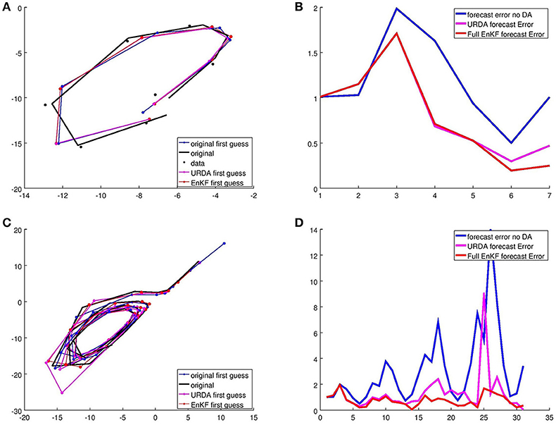
Figure 6. We show the results of the ultra rapid data assimilation in comparison with the ensemble Kalman square root filter for the Lorenz 1963 model for N = 8 assimilation steps and the reduced data case with observation operator H2. In (A,C), the black curve is the original, black dots are the observations. The mean of the analysis ensemble of the ultra rapid data assimilation URDA after k = 8 assimilation steps is shown in pink, where we need to note that here the information of the data is used to update the full curve at all points (i.e., the estimate of the past is updated as well. The red curve shows the analysis ensemble mean of the sequential ensemble Kalman square root filter. (B,D) show the sequential error curves of the analysis error for the two observed variables only, pink for URDA, red for the ensemble Kalman square root filter.
We analyse and investigate a ultra-rapid data assimilation scheme based on an ensemble square-root Kalman filter. Here, we have studied the analysis cycle, a preemptive forecasting step and also an ultra-rapid ensemble smoother.
For linear systems we have shown that the ultra-rapid data assimilation is equivalent to the full ensemble square-root filter. For non-linear systems, the Lorentz 63 system serves as a standard test case which is widely used within geophysics or the life sciences. We have carried out numerical tests of the URDA scheme, which shows highly encouraging results. For a significant number of assimilation and forecasting steps the URDA scheme shows a similar forecasting skill as the square-root filter with full model forecasts.
In particular, we have analyzed and tested the assimilation of observations which are influenced by a selection of state variables only, where the URDA scheme provides the possibility to touch only the variables of interest for the assimilation and preemptive forecasting or smoothing steps. This has very-high potential for many applications, where high-frequency analysis and/or forecasts need to be calculated, e.g., in the area of brain surgery in neuroscience or in nowcasting in geophysical applications.
This work aims to provide the basic theoretical inside and study a standard non-linear system of wide interest, the Lorenz 63 system. Initial tests on a real-world system in geophysics have been carried out in Etherton [25] and Madaus and Hakim[26]. Further work on error estimates for non-linear systems and the application of the method in neuroscience, biological systems or weather forecasting is still pending and will be our goal for the near future.
Ideas for the investigation by RP. Execution of the numerical calculations were performed by RP and CW. Writing the publication was done by RP and CW.
The authors declare that the research was conducted in the absence of any commercial or financial relationships that could be construed as a potential conflict of interest.
We thank Jeffrey Anderson from NCAR for the interesting discussions and pointing us to the paper of L. Madaus and G. Hakim. Furthermore we thank Z. Paschalidi and J. W. Acevedo Valencia for fruitful discussions on the topic, applications and further development of these ideas in the context of the projects Sinfony and Flottenwetterkarte at Deutscher Wetterdienst. This work was supported by the Deutscher Wetterdienst research program Innovation Programme for applied Researches and Developments (IAFE) in course of the SINFONY project.
1. ^Note that the calculation of this transform matrix takes place in ensemble space and is only a very small part of the total cost of the assimilation cycle and forecasting.
1. Park SK, Park L eds. Data Assimilation for Atmospheric, Oceanic and Hydrologic Applications (Vol. II). Berlin; Heidelberg: Springer-Verlag (2013).
2. Kalnay E. Atmospheric Modeling, Data Assimilation and Predictability. Cambridge: Cambridge University Press (2003).
4. Hamilton F, Berry T, Peixoto N, Sauer T. Real-time tracking of neuronal network structure using data assimilation. Phys Rev E (2013) 88:052715. doi: 10.1103/PhysRevE.88.052715
5. Nogaret A, Meliza CD, Margoliash D, Abarbanel HDI. Automatic construction of predictive neuron models through large scale assimilation of electrophysiological data. Sci Rep. (2016) 6:32749. doi: 10.1038/srep32749
6. Palmer T, Hagedorn R. Predictability of Weather and Climate. Cambridge: Cambridge University Press (2006).
7. Massimo B, Elias H, Lars I, Mike F. The evolution of the ECMWF hybrid data assimilation system. Q J R Meteorol Soc. (2015) 142:287–303. doi: 10.1002/qj.2652
8. Schraff C, Reich H, Rhodin A, Schomburg A, Stephan K, Periáñez A, et al. Kilometre-scale ensemble data assimilation for the COSMO model (KENDA). Q J R Meteorol Soc. (2016) 142:1453–72. doi: 10.1002/qj.2748
9. Jaisson P, DeVuyst F. Data assimilation and inverse problem for fluid traffic flow models and algorithms. Int J Numer Methods Eng. (2008) 76:837–61. doi: 10.1002/nme.2349
10. Fukuda D, Hong Z, Okamoto N, Ishida H. Data assimilation approach for traffic-state estimation and sensor location/spacing problems in an urban expressway. J Jpn Soc Civil Eng Ser D3. (2014) 70:I1041–50. doi: 10.2208/jscejipm.70.I_1041
11. Nantes A, Ngoduy D, Bhaskar A, Miska M, Chung E. Real-time traffic state estimation in urban corridors from heterogeneous data. Transport Res C Emerg Technol. (2016) 66:99–118. doi: 10.1016/j.trc.2015.07.005
12. Bocquet M, Pires CA, Wu L. Beyond gaussian statistical modeling in geophysical data assimilation. Monthly Weather Rev. (2010) 138:2997–3023. doi: 10.1175/2010MWR3164.1
13. Alberto C, Marc B, Laurent B, Geir E. Data assimilation in the geosciences: an overview of methods, issues, and perspectives. Wiley Interdiscipl Rev Clim Change (2018) 9:e535. doi: 10.1002/wcc.535
14. Dalety R. Atmospheric Data Analysis. Cambridge Atmospheric and Space Science Series. Cambridge: Cambridge University Press (1993).
15. Evensen G. Sequential data assimilation with a nonlinear quasi-geostrophic model using Monte Carlo methods to forecast error statistics. J Geophys Res Oceans (1994) 99:10143–62. doi: 10.1029/94JC00572
16. Hunt BR, Kostelich EJ, Szunyogh I. Efficient data assimilation for spatiotemporal chaos: A local ensemble transform Kalman filter. Physica D Nonlinear Phenomena (2007) 230:112–26. doi: 10.1016/j.physd.2006.11.008
17. Evensen G. Data Assimilation: The Ensemble Kalman Filter. Earth and Environmental Science. Heidelberg: Springer (2009).
18. Kalnay E, Hunt B, Ott E, Szunyogh I. Ensemble Forecasting and Data Assimilation: Two Problems With the Same Solution. Cambridge: Cambridge University Press (2006).
19. Freitag M, Potthast R. Synergy of inverse problems and data assimilation techniques. In: Cullen M, Freitag MA, Kindermann S, Scheichl R, editors. Large Scale Inverse Problems. vol. 13 of Radon Series on Computational and Applied Mathematics. Berlin: Walter de Gruyter (2013).
21. Gauthier P. Chaos and quadri-dimensional data assimilation: a study based on the Lorenz model. Tellus A (1992) 44:2–17. doi: 10.3402/tellusa.v44i1.14938
22. Evensen G. Advanced data assimilation for strongly nonlinear dynamics. Monthly Weather Rev. (1997) 125:1342–54.
23. Yang SC, Baker D, Li H, Cordes K, Huff M, Nagpal G, et al. Data assimilation as synchronization of truth and model: experiments with the three-variable lorenz system. J Atmos Sci. (2006) 63:2340–54. doi: 10.1175/JAS3739.1
24. Tandeo P, Ailliot P, Ruiz J, Hannart A, Chapron B, Cuzol A, et al. Combining Analog Method and Ensemble Data Assimilation: Application to the Lorenz-63 Chaotic System. In: Lakshmanan V, Gilleland E, McGovern A, Tingley M. Editors. Machine Learning and Data Mining Approaches to Climate Science. Cham: Springer International Publishing (2015). p. 3–12.
25. Etherton BJ. Preemptive forecasts using an ensemble kalman filter. Monthly Weather Rev. (2007) 135:3484–95. doi: 10.1175/MWR3480.1
26. Madaus LE, Hakim GJ. Rapid, short-term ensemble forecast adjustment through offline data assimilation. Q J R Meteorol Soc. (2015) 141:2630–42. doi: 10.1002/qj.2549
Keywords: data assimilation (DA), ensemble filter, preemtive forecast, Lorenz 1963 system, rapid update
Citation: Potthast R and Welzbacher CA (2018) Ultra Rapid Data Assimilation Based on Ensemble Filters. Front. Appl. Math. Stat. 4:45. doi: 10.3389/fams.2018.00045
Received: 16 July 2018; Accepted: 14 September 2018;
Published: 23 October 2018.
Edited by:
Wilhelm Stannat, Technische Universität Berlin, GermanyReviewed by:
Xin Tong, National University of Singapore, SingaporeCopyright © 2018 Potthast and Welzbacher. This is an open-access article distributed under the terms of the Creative Commons Attribution License (CC BY). The use, distribution or reproduction in other forums is permitted, provided the original author(s) and the copyright owner(s) are credited and that the original publication in this journal is cited, in accordance with accepted academic practice. No use, distribution or reproduction is permitted which does not comply with these terms.
*Correspondence: Roland Potthast, cm9sYW5kLnBvdHRoYXN0QGR3ZC5kZQ==
Disclaimer: All claims expressed in this article are solely those of the authors and do not necessarily represent those of their affiliated organizations, or those of the publisher, the editors and the reviewers. Any product that may be evaluated in this article or claim that may be made by its manufacturer is not guaranteed or endorsed by the publisher.
Research integrity at Frontiers
Learn more about the work of our research integrity team to safeguard the quality of each article we publish.