 Robert Beinert
 Gerlind Plonka
- 1Institut für Mathematik und Wissenschaftliches Rechnen, Karl-Franzens-Universität Graz, Graz, Austria
- 2Institut für Numerische und Angewandte Mathematik, Georg-August-Universität Göttingen, Göttingen, Germany
In this paper, we show that sparse signals f representable as a linear combination of a finite number N of spikes at arbitrary real locations or as a finite linear combination of B-splines of order m with arbitrary real knots can be almost surely recovered from intensity measurements up to trivial ambiguities. The constructive proof consists of two steps, where in the first step Prony's method is applied to recover all parameters of the autocorrelation function and in the second step the parameters of f are derived. Moreover, we present an algorithm to evaluate f from its Fourier intensities and illustrate it at different numerical examples.
1. Introduction
Phase retrieval problems occur in many scientific fields, particularly in optics and communications. They have a long history with rich literature regarding uniqueness of solutions and existence of reliable algorithms for signal reconstruction, see e.g., [1] and references therein. Usually, the challenge in solving one-dimensional phase retrieval problems is to overcome the strong ambiguousness by determining appropriate further information on the solution signal. Previous literature on characterization of ambiguities of the phase retrieval problem with given Fourier intensities is often concerned with the discrete problem, where a signal x in ℝN or ℂN has to be recovered. For an overview on the occurring trivial and non-trivial ambiguities in the discrete setting we refer to our survey [2]. The behavior of the solution set under additional constraints has been studied for instance in Beinert and Plonka [2, 3], Beinert [4, 5].
1.1. Contribution of This Paper
In this paper, we consider the continuous one-dimensional sparse phase retrieval problem to reconstruct a complex-valued signal from the modulus of its Fourier transform. Applications of this problem occur in electron microscopy, wave front sensing, laser optics [6, 7] as well as in X-ray crystallography and speckle imaging [8]. For the posed problem, we will show that for sparse signals the given Fourier intensities are already sufficient for an almost sure unique recovery, and we will give a construction algorithm to recover f.
We assume that the sparse signal is either of the form
or, for m > 0,
with , Tj ∈ ℝ for j = 1, …, N, where δ denotes the Delta distribution, and Bj, m is the B-spline of order m being determined by the (real) knots Tj < Tj+1 < … < Tj+m. We want to recover these signals from the Fourier intensities and will show that only (N2) samples are needed to recover f, i.e., all coefficients , j = 1, …, N and knots Tj, j = 1, …, N + m, almost surely up to trivial ambiguities. The proposed procedure is constructive and consists in two steps. In a first step, we employ Prony's method to determine the coefficients and frequencies of the exponential sum . These frequencies are of the form Tj − Tk with j, k ∈ {1, …, N + m}. If these knot differences Tj − Tk are pairwise different for j ≠ k, then we can use this information in a second reconstruction step to compute the knots Tj and the coefficients cj, and thus the desired signal.
1.2. Related Work on Sparse Phase Retrieval
While the general phase retrieval problem has been extensively studied for a long time, the special case of sparse phase retrieval grew to a strongly emerging field of research only recently, particularly often connected with ideas from compressed sensing. Most of the papers consider a discrete setting, where the N-dimensional real or complex k-sparse vector x has to be reconstructed from measurements of the more general form with vectors aj forming the rows of a measurement matrix A ∈ ℂM×N. The needed number M of measurements depends on the sparsity k.
If A presents rows of a Fourier matrix, this setting is close to the sparse phase retrieval problem considered in optics, see e.g.,[9]. Here the problem is first rewritten as (non-convex) rank minimization problem, then a tight convex relaxation is applied and the optimization problem is solved by a re-weighted l1-minimization method. The related approach in Eldar et al. [10] employs the magnitudes of the short-time Fourier transform and applies the occurring redundancy for unique recovery of the desired signal. A corresponding reconstruction algorithm is then based on an adaptation of the GESPAR algorithm in Shechtman et al. [11].
In Li and Voroninski [12], the measurement matrix A is taken with random rows and the PhaseLift approach [13] leads to a convex optimization problem that recovers the sparse solution with high probability. Employing a thresholded gradient descent algorithm to a non-convex empirical risk minimization problem that is derived from the phase retrieval problem, Cai et al. [14] have established the minimax optimal rates of convergence for noisy sparse phase retrieval under sub-exponential noise.
Other papers rely on the compressed sensing approach to construct special frame vectors aj to ensure uniqueness of the phase retrieval problem with high probability, where the number of needed vectors is (k), see e.g., [15–17].
We would like to emphasize that all approaches employing general or random measurement matrices in phase retrieval are quite different in nature from our phase retrieval problem based on Fourier intensity measurements. In this paper, we want to stick on considering Fourier intensity measurements because of their particular relevance in practice.
Early attempts to exploit sparsity of a discrete signal for unique recovery using Fourier intensities go back to unpublished manuscripts by Yagle [18, 19], where a variation of Prony's method is applied in a non-iterative algorithm to sparse signal and image reconstruction. Unfortunately, the algorithm proposed there not always determines the signal support correctly.
The continuous one-dimensional phase retrieval problem has been rarely discussed in the literature, see [5, 8, 20–22]. In the preprint [8], the authors also considered the recovery of sparse continuous signals of the form (1.1). However, in that paper the sparse phase retrieval problem is in turn transferred into a turnpike problem that is computationally expensive to solve. Moreover there exist cases, where a unique solution cannot be found, see [23]. Our method circumvents this problem by proposing an iterative procedure to fix the signal support (resp. the knots of the signal represented as a B-spline function) where the corresponding signal coefficients are evaluated simultaneously.
1.3. Organization of This Paper
In Section 2, we shortly recall the mathematical formulation of the considered sparse phase retrieval problem and the notion of trivial ambiguities of the phase retrieval problem that always occur.
Section 3 is devoted to the special case of phase retrieval for signals of the form (1.1). Using Prony's method, we give a constructive proof for the unique recovery of the N-sparse signal f up to trivial ambiguities using 3/2N(N−1)+1 Fourier intensity measurements. Here we have to assume that the knot differences Tj − Tk are pairwise different.
In Section 4, the ansatz is generalized to the unique recovery of spline functions of the form (1.2) where we need to employ 3/2(N + m)(N + m − 1) + 1 Fourier intensity measurements. In Section 5, we present an explicit algorithm for the considered sparse phase retrieval problem and illustrate it at different examples.
2. Trivial Ambiguities of the Phase Retrieval Problem
We wish to recover an unknown complex-valued signal f : ℝ → ℂ of the form (1.1) or (1.2) with compact support from its Fourier intensity given by
For the spike function in (1.1), we interpret the Fourier integral in (2.1) in a distributional sense, i.e., . Unfortunately, the recovery of the signal f is complicated because of the well-known ambiguousness of the phase retrieval problem. Transferring [2, Proposition 2.1] to our setting, we can recover f only up to the following ambiguities, which immediately follow from the properties of the Fourier transform.
Proposition 2.1. Let f be a signal of the form (1.1) or a non-uniform spline function of the form (1.2). Then
(i) the rotated signal eiα f for α ∈ ℝ,
(ii) the time shifted signal f(· − t0) for t0 ∈ ℝ,
(iii) and the conjugated and reflected signal
have the same Fourier intensity .
Although the ambiguities in Proposition 2.1 always occur, they are of minor interest because of their close relation to the original signal. For this reason, we call ambiguities caused by rotation, time shift, conjugation and reflection, or by combinations of these trivial. In the following, we will show that for the considered sparse signals the remaining non-trivial ambiguities only occur in rare cases.
3. Phase Retrieval for Distributions with Discrete Support
Initially, we restrict ourselves to the recovery of signals f of the form (1.1) with complex-valued coefficients , spike locations T1 < ⋯ < TN, and Fourier transform.
The known squared Fourier intensity can be represented by
Thus, in order to recover f being determined by the coefficients and the knots Tj ∈ ℝ, j = 1, …, N, we will first recover the differences of the frequencies Tj − Tk and the corresponding products of coefficients in (3.1) and then derive the desired parameters of f in a second step.
3.1. First Step: Parameter Recovery by Prony's Method
Let us assume that the knot differences Tj − Tk in (3.1) are pairwise different for j ≠ k. The squared Fourier intensity can then be written in the form
where we assume that the frequencies τℓ, ℓ = −N(N−1)/2, …, N(N−1)/2 are ordered by size. Obviously, the frequency differences τℓ satisfy τ−ℓ = −τℓ. Further, each τℓ > 0 corresponds to a difference Tj − Tk for some j > k, and the related coefficient γℓ then equals to . For the zero frequency τ0 = 0, we have .
In the first step, we want to recover all frequencies τℓ and the corresponding coefficients γℓ, ℓ = 0, …, N(N−1)/2 of P(ω). However, at this stage, the bijective mapping between ℓ > 0 and (j, k) with j > k such that τℓ = Tj − Tk will be still unknown and needs to be found in a second reconstruction step. In order to recover the frequency differences τℓ and the unknown coefficients γℓ from the exponential sum (3.2) we employ Prony's method [24, 25].
Let h > 0 be chosen such that hτℓ < π for all ℓ = 1, …, N(N−1)/2. Using the intensity values , k = 0, …, 2N(N − 1) + 1, the unknown parameters γℓ and τℓ in (3.2) can be determined by exploiting the algebraic Prony polynomial Λ(z) defined by
where λk denote the coefficients in the monomial representation of Λ(z). Obviously, Λ(z) is always a monic polynomial, which means that λN(N−1)+1 = 1.
Using the definition of the Prony polynomial Λ(z) in (3.3), we observe that
for m = 0, …, N(N − 1). Consequently, the vector of remaining coefficients of the Prony polynomial Λ(z) can be determined by solving the system of linear equations
with and . Since the Hankel matrix H can be written as
with the Vandermonde matrix , the system of linear equations (3.4) possesses a unique solution if and only if the unimodular values differ pairwise for ℓ = −N(N−1)/2, …, N(N−1)/2. This assumption has been ensured by choosing an h such that hτℓ ∈ (−π, π), since the τℓ had been supposed to be pairwise different.
Knowing the coefficients λk of Λ(z), we can determine the unknown frequencies τℓ by evaluating the roots of the Prony polynomial (3.3). The coefficients γℓ can now be computed by solving the over-determined equation system
with a Vandermonde-type system matrix.
The procedure summarized above is Prony's method, adapted to the non-negative exponential sum P(ω) in (3.2). In the numerical experiments in Section 5, we will apply the approximate Prony method (APM) in Potts and Tasche [26]. APM is based on the above considerations but it is numerically more stable and exploits the special properties and τ−ℓ = −τℓ for ℓ = 0, …, N(N−1)/2.
Let us now investigate the question, how many intensity values are at least necessary for the recovery of P(ω) in (3.2). Counting the number of unknowns of P(ω) in (3.2), we only need to recover the 3/2N(N − 1) + 1 real values γ0 and Re γℓ, Im γℓ, τℓ, for ℓ = 1, …N(N−1)/2. We will show now that using the special structure of the real polynomial P(ω) in (0.2) and of the Prony polynomial Λ(z) in (0.3), we indeed need only 3/2N(N − 1) + 1 exact equidistant real measurements P(kh), k = 0, …, 3/2N(N − 1) to recover all parameters determining P(ω). This can be seen as follows.
Reconsidering Λ(z) in (3.3) with τ0 = 0 and τℓ = −τ−ℓ, we obtain
where all occurring coefficients λk are real. Moreover, since
is antisymmetric, it follows that
and particularly λN(N−1)+1 = −λ0 = 1. In order to determine the unknown coefficients λk, k = 1, …, N(N−1)/2 of
we employ (3.2) and observe that for m = 0, …, N(N−1)/2 − 1,
Therefore, the vector of unknown coefficients can be evaluated from the system
The frequency differences τℓ are then extracted from the zeros of Λ(z), and the coefficients γℓ, ℓ = 0, …, N(N−1)/2, are computed as in (3.5) but with k = 0, …, 3/2N(N − 1).
3.2. Second Step: Unique Signal Recovery
Having determined the frequency differences τℓ as well as the corresponding coefficients γℓ of (3.2), we want to reconstruct the parameters Tj and , j = 1, …, N, of f in (1.1) in a second step.
Theorem 3.1. Let f be a signal of the form (1.1), whose knot differences Tj − Tk differ pairwise for j, k ∈ {1, …, N} with j ≠ k, and whose coefficients satisfy . Further, let h be a step size such that h(Tj − Tk) ∈ (−π, π) for all j, k. Then f can be uniquely recovered from its Fourier intensities with ℓ = 0, …, 3/2N(N − 1) up to trivial ambiguities.
Proof. Applying Prony's method to the given data , we can compute the frequency differences τℓ and the related coefficients γℓ of the squared Fourier intensity (3.2). We denote by the list of obtained positive frequencies ordered by size. Now, we need to recover the mapping ℓ → (j, k) such that τℓ = Tj − Tk, where we can assume that j > k for ℓ > 0.
Obviously, the maximal distance τN(N−1)/2 is now equal to the length TN − T1 of the unknown f in (1.1). Due to the trivial shift ambiguity, we can assume without loss of generality that T1 = 0 and TN = τN(N−1)/2. Further, the second largest distance τ(N(N−1)/2)−1 corresponds either to TN−1 − T1 or to TN − T2. Due to the trivial reflection and conjugation ambiguity, we can assume that TN−1 = TN−1 − T1 = τ(N(N−1)/2)−1. By definition, there exists a in our sequence of parameters such that , and is hence equal to the knot difference TN − TN−1. Thus, we obtain
These equations lead us to
and thus to
Since f can only be recovered up to a global rotation, we can assume that is real and non-negative, which allows us to determine the coefficients , , and in a unique way.
Having fixed TN = TN − T1 = τN(N−1)/2 and TN−1 = TN−1−T1 = τ(N(N−1)/2)−1 we notice that the third largest distance τ(N(N−1)/2)−2 is either equal to TN−T2 or to TN−2−T1 = TN−2. As before, there exists a frequency such that .
Case 1: If τ(N(N−1)/2)−2 = TN−T2, then we have
with the related coefficient . Moreover, we have such that
Case 2: If τ(N(N−1)/2)−2 = TN−2−T1, then we have
with the related coefficient and . Thus,
However, only one of the two equalities in (3.6) and (3.7) can be true, since if both were true then and lead to
contradicting the assumption that . Consequently, either the equation in (3.6) or the equation in (3.7) holds true and we can either determine T2 with or TN−2 with . Removing all frequency differences τℓ from the sequence of distances that correspond to the differences Tj − Tk of the recovered knots, we can repeat this approach to find the remaining coefficients and knots of f inductively. □
If we identify the space of complex-valued signals of the form (1.1) with the real space ℝ3N, the condition that two knot differences Tj1−Tk1 and Tj2−Tk2 are equal for fixed indices j1, j2, k1, and k2 defines a hyperplane with Lebesgue measure zero. An analogous observation follows for the condition . The signals excluded in Theorem 3.1 hence form a negligible null set.
Corollary 3.2. Almost all signals f in (1.1) can be uniquely recovered from their Fourier intensities up to trivial ambiguities.
Remark 3.3. 1. Since the proof of Theorem 3.1 is constructive, it can be used to recover an unknown signal (1.1) analytically and numerically. If the number N of spikes is known beforehand then the assumption of Theorem 3.1 can be simply checked during the computation. If the assumption regarding pairwise different distances Tj − Tk is not satisfied, then the application of Prony's method in the first step yields less than N(N − 1) + 1 pairwise distinct frequency differences τℓ. The second assumption can be verified in the second step, where , , and are evaluated.
2. A similar phase retrieval problem had been transferred to a turnpike problem in Ranieri et al. [8]. The turnpike problem deals with the recovery of the knots Tj from an unlabeled set of distances. Although this problem is solvable under certain conditions, a backtracing algorithm can have exponential complexity in the worst case, see [27].
4. Retrieval of Spline Functions with Arbitrary Knots
In this section, we generalize our findings to spline functions of order m ≥ 1. Let us recall that the B-splines Bj, m in (1.2) being generated by the knot sequence T1 < ⋯ < TN+m are recursively defined by
with
see for instance [28, p. 131]. Further, we notice that for 0 ≤ k ≤ m−2 the kth derivative of the spline f in (1.2) is given by
where the coefficients are recursively defined by
with the convention that , see [28, p. 139]. For k = m − 1, Equation (4.1) coincides with a step function, i.e., with the right derivative of the linear spline f(m−2). Further, in a distributional manner, the mth derivative of f is given by
with the coefficients
and the Dirac delta distribution δ.
Applying the Fourier transform to (4.2), we now obtain
and thus
Since the exponential sum on the right-hand side of (4.4) has exactly the same structure as the exponential sum in (3.2), we can immediately generalize Theorem 3.1 by considering
Theorem 4.1. Let f be a spline function of the form (1.2) of order m, whose knot distances Tj − Tk differ pairwise for j, k ∈ {1, …, N + m} with j ≠ k, and whose coefficients satisfy . Further, let h be a step size such that h(Tj − Tk) ∈ (−π, π) for all j, k. Then f can be uniquely recovered from its Fourier intensities with ℓ = 0, …, (N + m)(N + m − 1) up to trivial ambiguities.
Proof. The statement can be established by proceeding in the same manner as in Section 3. First we apply Prony's method to the given samples with ℓ = 0, …, (N + m)(N + m − 1) in order to determine the coefficients and frequencies of P(ω) in (4.5). In a second step, the values and Tj in (4.3) can be determined analytically as discussed in Theorem 3.1. Reversing the definition of , we can finally compute the unknown coefficients by
and
with and , which finishes the proof. □
Corollary 4.2. Almost all spline functions f of order m in (1.2) can be uniquely recovered from their Fourier intensities || up to trivial ambiguities.
5. Numerical Experiments
Since the proofs of Theorem 3.1 and Theorem 4.1 are constructive, they can be straightforwardly transferred to numerical algorithms to recover a spline function from its Fourier intensity. However, Prony's classical method introduced in subsection 3.1 is numerically unstable with respect to inexact measurements and to frequencies lying close together. For this reason, there are numerous approaches to improve the classical method. In order to verify Theorem 3.1 and Theorem 4.1 numerically, we apply the so-called approximate Prony method (APM) proposed by Potts and Tasche [26, Algorithm 4.7] for recovery of parameters of an exponential sum of the form
with τℓ = −τ−ℓ and . The algorithm can be summarized as follows, where the exact number 2M + 1 of the occurring frequencies in (5.1) needs not be known beforehand.
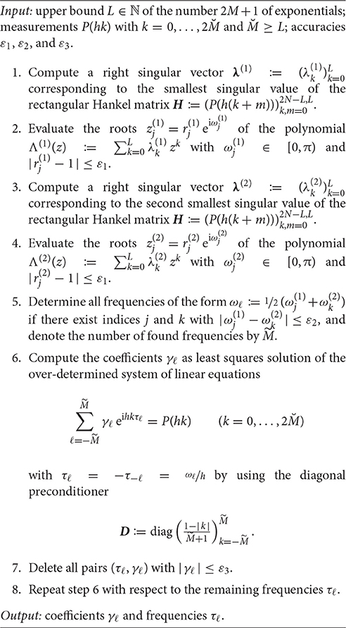
Algorithm 5.1 Approximate Prony method [26]
A second adaption of the proof of Theorem 4.1 concerns the reconstruction of the coefficients from the recovered coefficients . In order to describe the relation between the coefficients as system of linear equations, we define the rectangular matrices C(m−k) ∈ ℝ(N+k−1) × (N+k) for k = 0, …, m−1 elementwise by
and
Then, the recursion between the coefficients and can be stated as
where we use the coefficient vectors . Instead of computing the coefficients stepwise from left to right, we can determine the coefficients by solving the over-determined system of linear equations
With these modifications, we recover a spline function of order m from its Fourier intensity by the following algorithm.
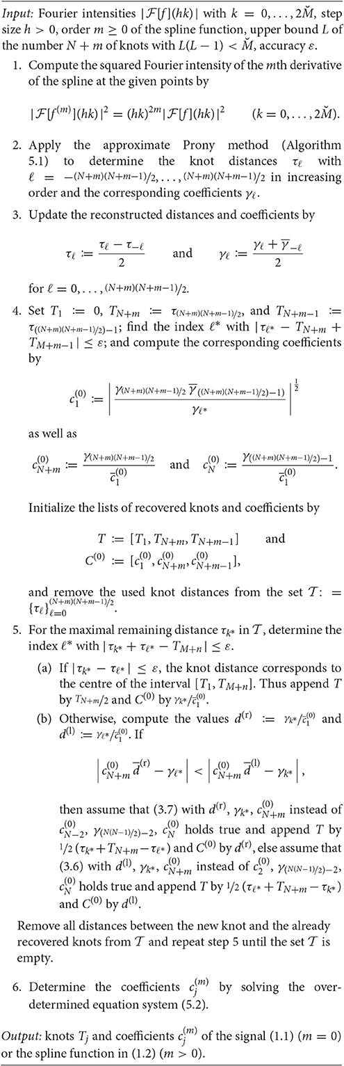
Algorithm 5.2 Phase retrieval
Example 5.1. In the first numerical example, we consider a spike function as in (1.1) with 15 spikes. More precisely, the locations Tj and the coefficients of the true spike function f are given in Table 1. In order to recover f from the Fourier intensity measurements with ℓ = 0, …, 1000, we apply Algorithm 2 with the accuracies ε : = 10−3, , , and . In order to ensure that h(Tj − Tk) ∈ (−π, π) as assumed in Theorem 3.1, we chose h : = 0.95(T15−T1)/π. The results of the phase retrieval algorithm and the absolute errors of the knots and coefficients of the recovered spike function are shown in Figure 1. Although the approximate Prony method has to recover 211 knot differences, the knots and coefficients of f are reconstructed very accurately. ○
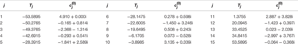
Table 1. Knots Tj and coefficients of the spike function in Example 5.1.
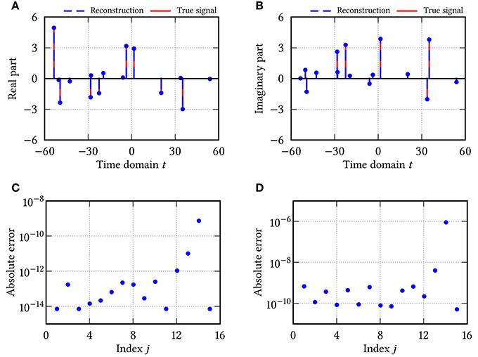
Figure 1. Results of Algorithm 5.2 for the spike function in Example 5.1. (A) Real part of the recovered and true spike function. (B) Imaginary part of the recovered and true spike function. (C) Absolute error of the recovered knots. (D) Absolute error of the recovered coefficients.
Example 5.2. In the second example, we consider the piecewise quadratic spline function f of order m = 3 as in (1.2) with N = 7 coefficients and N + m = 10 knots as given in Table 2. To recover f from its Fourier intensity measurements with ℓ = 0, …, 400 and with h = 0.95(T10−T1)/π, we again apply Algorithm 2. As accuracies for the phase retrieval algorithm and the approximate Prony method, we choose ε : = 10−3, , , and . In Figure 2, the recovered function is compared with the true signal. Again, the reconstructed knots and coefficients have only very small absolute errors. ○
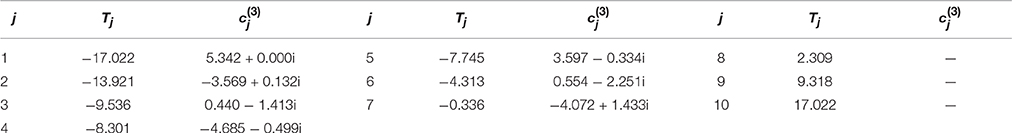
Table 2. Knots Tj and coefficients of the spline function in Example 5.2.
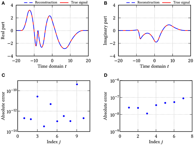
Figure 2. Results of Algorithm 5.2 for the spline function in Example 5.2. (A) Real part of the recovered and true spline function. (B) Imaginary part of the recovered and true spline function. (C) Absolute error of the recovered knots. (D) Absolute error of the recovered coefficients.
6. Summary and Discussion
In this paper, we have presented a novel approach to recover a sparse continuous-time signal f from finitely many samples of its Fourier intensity .
While the general phase retrieval problem is highly ambiguous, the assumed sparsity of the unknown signal surmounts this problem and guarantees uniqueness of the phase retrieval problem up to trivial ambiguities. In many applications, the sparsity assumption arises in a natural manner. For instance, the positions of stars in astronomy [29] or the positions of atoms in a molecule in crystallography [30] correspond to a sparse spike functions.
Here, we have assumed that f is a finite linear combination of spikes or B-splines with arbitrary knots. The new approach consists of two steps, where we have applied Prony's method in a first step to determine the knot differences from the exponential sum . Based on this information, we have derived a method to recover the unknown knots and coefficients of f step by step. The significant benefit over the previous approach in Ranieri et al. [8] is the exploitation of the coefficients of , which allows the simultaneous recovery of the knots and coefficients of the true signal f always with polynomial complexity. Our method works for all signals whose knot differences are pairwise distinct. Therefore, almost every structured function of the form (1.1) or (1.2) can be uniquely recovered from its Fourier intensity up to trivial ambiguities. In the numerical examples, we show that our methods behaves well in the noise-free setting. Our work is a first step to phase retrieval of spline functions and raises several theoretical and numerical questions.
The considered phase retrieval problem employs Fourier transform intensities. For spike functions, the proposed method can be easily extended to measurements from a canonical linear transform like the Fresnel or the fractional Fourier transform, since these transforms merely correspond to a non-linear modulation of the coefficients, cf. [31]. The phase retrieval problem of spline functions in Section 4 is essentially based on formula (4.3) on the representation of function derivatives in Fourier domain. This property does not generally hold for canonical linear transforms.
The sensitivity of our reconstruction algorithm with respect to noisy measurements depends on the approximate Prony method. In fact, the desired frequency differences possess a very special structure and have to satisfy certain side conditions. For example, the sum of two frequency differences Tj − Tk and Tℓ − Tj is again a frequency difference Tℓ − Tk. For strongly disturbed measurements, the recovered frequency differences obtained by the approximate Prony method may not satisfy this special structure, and the second reconstruction step of our method cannot be applied directly. Therefore, it would be interesting to study, how the approximate Prony method can be modified by incorporating the additional structure information.
Author Contributions
All authors listed, have made substantial, direct and intellectual contribution to the work, and approved it for publication.
Conflict of Interest Statement
The authors declare that the research was conducted in the absence of any commercial or financial relationships that could be construed as a potential conflict of interest.
Acknowledgments
We thank the referees for many helpful comments and suggestions to improve the representation of the results in this paper. Further, the first author gratefully acknowledges the funding of this work by the Austrian Science Fund (FWF) within the project P 28858, and the second author the funding by the German Research Foundation (DFG) within the project PL 170/16-1 and within the CRC 755. The Institute of Mathematics and Scientific Computing of the University of Graz, with which the first author is affiliated, is a member of NAWI Graz (http://www.nawigraz.at/).
References
1. Shechtman Y, Eldar YC, Cohen O, Chapman HN, Miao J, Segev M. Phase retrieval with application to optical imaging: a contemporary overview. IEEE Signal Process Magaz. (2015) 32:87–109. doi: 10.1109/MSP.2014.2352673
2. Beinert R, Plonka G. Ambiguities in one-dimensional discrete phase retrieval from Fourier magnitudes. J Fourier Anal Appl. (2015) 21:1169–98. doi: 10.1007/s00041-015-9405-2
3. Beinert R, Plonka G. Enforcing uniqueness in one-dimensional phase retrieval by additional signal information in time domain Appl Comput Harm Anal. (2017). arXiv:1604.04493v1
4. Beinert R. Non-negativity constraints in the one-dimensional discrete-time phase retrieval problem. Inform Infer. (2017). arXiv:1605.05482
5. Beinert R. One-dimensional phase retrieval with additional interference measurements; 2017. Results Math. (2017). arXiv:1604.04489v1
6. Seifert B, Stolz H, Tasche M. Nontrivial ambiguities for blind frequency-resolved optical gating and the problem of uniqueness. J Opt Soc Am B (2004) 21:1089–97. doi: 10.1364/JOSAB.21.001089
7. Seifert B, Stolz H, Donatelli M, Langemann D, Tasche M. Multilevel Gauss-Newton methods for phase retrieval problems. J Phys Math General (2006) 39:4191–206. doi: 10.1088/0305-4470/39/16/007
8. Ranieri J, Chebira A, Lu YM, Vetterli M. Phase retrieval for sparse signals: uniqueness conditions (2013). arXiv:1308.3058v2
9. Jaganathan K, Oymak S, Hassibi B. Sparse Phase Retrieval: convex Algorithms and Limitations. In: IEEE International Symposium on Information Theory Proceedings (ISIT), Piscataway, NY (2013). p. 1022–6.
10. Eldar YC, Sidorenko P, Mixon DG, Barel S, Cohen O. Sparse phase retrieval from short-time Fourier measurements. IEEE Signal Process Lett. (2015) 22:638–42. doi: 10.1109/LSP.2014.2364225
11. Shechtman Y, Beck A, Eldar YC. GESPAR: efficient phase retrieval of sparse signals. IEEE Trans Signal Process. (2014) 62:928–38. doi: 10.1109/TSP.2013.2297687
12. Li X, Voroninski V. Sparse signal recovery from quadratic measurements via convex programming. SIAM J Math Anal. (2013) 45:3019–33. doi: 10.1137/120893707
13. Candès EJ, Strohmer T, Voroninski V. PhaseLift: exact and stable signal recovery from magnitude measurements via convex programming. Commun Pure Appl Math. (2013) 66:1241–74. doi: 10.1002/cpa.21432
14. Cai T, Tony Li X, Ma Z. Optimal rates of convergence for noisy sparse phase retrieval via thresholded Wirtinger Flow. Ann Statist. (2016) 44:2221–51. doi: 10.1214/16-AOS1443
15. Wang Y, Xu Z. Phase retrieval for sparse signals. Appl Comput Harm Anal. (2014) 37:531–44. doi: 10.1016/j.acha.2014.04.001
16. Ohlsson H, Eldar YC. On conditions for uniqueness in spare phase retrieval. In: Proceedings : ICASSP 14 : IEEE International Conference on Acoustics, Speech, and Signal Processing. Florence: IEEE (2014). p. 1841–5.
17. Iwen M, Viswanathan A, Wang Y. Robust sparse phase retrieval made easy. Appl Comput Harm Anal. (2017) 42:135–42. doi: 10.1016/j.acha.2015.06.007
18. Yagle AE. Non-iterative superresolution phase retrieval of sparse images without support constraints. Available online at: http://web.eecs.umich.edu/~aey/sparse/sparse8.pdf
19. Yagle AE. Recovery of K-Sparse Non-Negative Signals From K DFT Values and Their Conjugates. Available online at: http://web.eecs.umich.edu/~aey/sparse/sparse14.pdf
20. Walther A .The question of phase retrieval in optics. Opt Acta Int J Opt. (1963) 10:41–9. doi: 10.1080/713817747
21. Hofstetter EM. Construction of time-limited functions with specified autocorrelation functions. IEEE Trans Inf Theory (1964) 10:119–26. doi: 10.1109/TIT.1964.1053648
22. Beinert R, Plonka G. Ambiguities in one-dimensional phase retrieval of structured functions. Proc Appl Math Mech. (2015) 15:653–4. doi: 10.1002/pamm.201510316
24. Hildebrand FB Introduction to Numerical Analysis. 2nd Edn., New York: Dover Publications (1987).
25. Plonka G, Tasche M. Prony methods for recovery of structured functions. GAMM-Mitteilungen (2014) 37:239–58. doi: 10.1002/gamm.201410011
26. Potts D, Tasche M. Parameter estimation for exponential sums by approximate prony method. Signal Process. (2010) 90:1631–42. doi: 10.1016/j.sigpro.2009.11.012
27. Lemke P, Skiena SS, Smith WD. Reconstructing sets from interpoint distances. In: Aronov B, Basu S, Pach J, Sharir M, editors. Discrete and Computational Geometry. Berlin; Heidelberg: Springer (2003). p. 597–631.
29. Bruck YM, Sodin LG. On the ambiguity of the image reconstruction problem. Opt Commun. (1979) 30:304–8. doi: 10.1016/0030-4018(79)90358-4
30. Millane RP. Phase retrieval in crystallography and optics. J Opt Soc Am A (1990) 7:394–411. doi: 10.1364/JOSAA.7.000394
Keywords: sparse phase retrieval, sparse signals, non-uniform spline functions, finite support, Prony's method
AMS Subject classifications: 42A05, 94A08, 94A12.
Citation: Beinert R and Plonka G (2017) Sparse Phase Retrieval of One-Dimensional Signals by Prony's Method. Front. Appl. Math. Stat. 3:5. doi: 10.3389/fams.2017.00005
Received: 10 January 2017; Accepted: 21 March 2017;
Published: 10 April 2017.
Edited by:
Daniel Potts, Technische Universität Chemnitz, GermanyReviewed by:
Dirk Langemann, Technische Universität Braunschweig, GermanyMartin Ehler, University of Vienna, Austria
Copyright © 2017 Beinert and Plonka. This is an open-access article distributed under the terms of the Creative Commons Attribution License (CC BY). The use, distribution or reproduction in other forums is permitted, provided the original author(s) or licensor are credited and that the original publication in this journal is cited, in accordance with accepted academic practice. No use, distribution or reproduction is permitted which does not comply with these terms.
*Correspondence: Gerlind Plonka, plonka@math.uni-goettingen.de