Modelling individual plants’ growth: competition of Viola arvensis and wheat

Introduction: Competition by weeds is a severe threat to agricultural crops. While these days the broadcast of herbicides over the entire field is common praxis, new technologies promise to reduce chemical output by reducing the area sprayed. The maximum precision would be a single plant treatment. This precision will allow a single plant management, which requires single plant management decisions, which is far beyond the possibilities of current praxis. A plant specific management decision can only be made on the basis of a model simulation.

Materials and methods: A simulation model was developed to evaluate the effect of spatially explicit weed management covering interaction between single plants. The governing equations consist of coupled nonlinear differential equations for growth and competition of crop and weed plants in a spatial setting i.e. a coordinate is assigned to each plant. The mutual interaction is determined by the parameters strength and range of competition. Furthermore, an experiment was carried out parallel to the development of the model involving wheat and Viola arvensis (Murr.), in which coordinates and growth curves for a large number of plants (~600) were recorded allowing for a reasonable parameterization of the model.

Results and discussion: The model is able to evaluate spatially explicit management measures such as weed strip control based on the height growth of single plants. The model is capable of evaluating a variety of control measures such as the frequency and spatial allocation of treatments. In particular, the effect of the width of a treatment zone around the rows of the crop was simulated.

Conclusion: In future, the developed model could be extended to a decision support system for single plant weed management. Making decisions plant-by-plant, allows to orchestrate the weed management in a way that takes into account competing goals in plant protection: yield and biodiversity.

1 Introduction

Already in 1981 the German minister for agriculture stated that chemical plant protection is criticized by the society (Niemann, 1981). This criticism has not changed since then. Despite this long history, weed management in modern agriculture still relies on the large-scale application of herbicides. Meanwhile, techniques that allow a more precise, a site-specific weed management are available. These techniques allow severe savings in herbicides while maintaining high weed control. There are even first devices on the market that allow single plant control for weeds, which is the highest possible precision. Beside the higher efficiency, it was claimed that the precision is good for environment and biodiversity, but a proof is lacking to a large extend.

The effect of site-specific weed management (SSWM) on biodiversity can be severe (Hamouz et al., 2014). Weeds as a basis for biodiversity on agricultural fields (Marshall et al., 2003; Petit et al., 2011) might be locally spared to provide resources for higher trophic levels (Storkey and Westbury, 2007). This could be done on areas on the field with low yield expectation or difficult accessibility, requiring extensive planning for specific fields. Extending this approach to single-plant measures, a decision whether or not to control a specific plant can be made for various reasons, such as competitiveness, nice looking flowers, or biodiversity.

Site-specific weed management reduces the necessary amount of herbicides depending on the local weed density (Fernández-Quintanilla et al., 2020). Therefore, weeds in the field must be detected and mapped. In recent years, the technology required has greatly improved (Huang et al., 2018; Anul Haq, 2022). A management plan can be generated using economic thresholds for site-specific weed control (Keller et al., 2014). To do that an estimate of the effect on crop yield of weed control is necessary. First approaches established fixed threshold densities for specific weed species or groups using simple models (Gerowitt and Heitefuss, 1990). While thresholds for densities are an easy way to make decisions in field, using the underlying models directly is more flexible. Plant height was, and still is, a parameter recognized as a possibility to estimate the crop yield. In contrast to plant biomass, plant height is easy to measure in a field. Therefore, modelling the growth of plant height to estimate effects on crop yield is therefore an excellent pragmatic choice. For a longer period simulation models were rarely developed (Jiang et al., 2020). However, some studies worked on it. For example (Confalonieri et al., 2011) compared different models for the height of rice and similarly Jiang et al. (2020) compared different models for plant height of winter wheat under water stress. Maize growth was simulated with a multi parameter approach using LAI and plant height beside other parameters (Liao et al., 2023). Fang et al. (2022) used the Gompertz as well as the logistic function to model the growth of tomatos. Logistic models were used to model the growth of different crops by (Liu et al., 2022) as well. All the functions and approaches described do not include interactions between single plants and thus are not suitable to cover single plant management. The mechanistic FlorSys model “virtual field” can partly cover this aspect (Colbach et al., 2021). While FLORSYS is very powerful, it is complex and requires a large number of parameters (Colas et al., 2021). An alternative approach is the use of coupled differential equations, which have a long tradition for modelling plant-plant interactions (e.g. Damgaard et al., 2002). They are best suited of capturing the growth dynamics with a limited number of parameters. However, differential equations are deterministic.

The aim of the presented work was to develop a comprehensive model with only few state variables and with a parsimonious parameter set, capable of simulating the spatio-temporal management of weed populations. We base our model on logistic growth functions, because it has proven to be effective in modelling the plant height growth in diverse settings (Jiang et al., 2020; Fang et al., 2022; Liu et al., 2022). For plant-plant interactions, we used coupled logistic equations. The model approach chosen in our work therefore implies differential equations with stochastic elements. These concern (1) individual growth parameters, (2) spatially random distribution of weeds and (3) random emergence of weeds. In addition, a field experiment was conducted in which individual growth curves of the crop wheat and the weed plant Viola arvensis (Murr.) were measured at precisely mapped locations to fit the model structure and generate data for parameterization.

2 Materials and methods

2.1 Simulation model

2.1.1 General concept

The model structure combines individual based models with stochastic elements. Referring to individual plants entails a fixed location of every plant in space. Furthermore, the interaction between plants depends on their distance. The spatial configuration of the crop is fixed by the cultivation, whereas weeds emerge randomly from the seedbank (Figure 1). The growth of every individual plant is modelled by a differential equation taking into account the mutual competition between and within species. The management is restricted to specific positions, thus allows for single-plant measures. The full model combining all three parts, the germination, the growth and the management, is described in Equation 12.

Figure 1

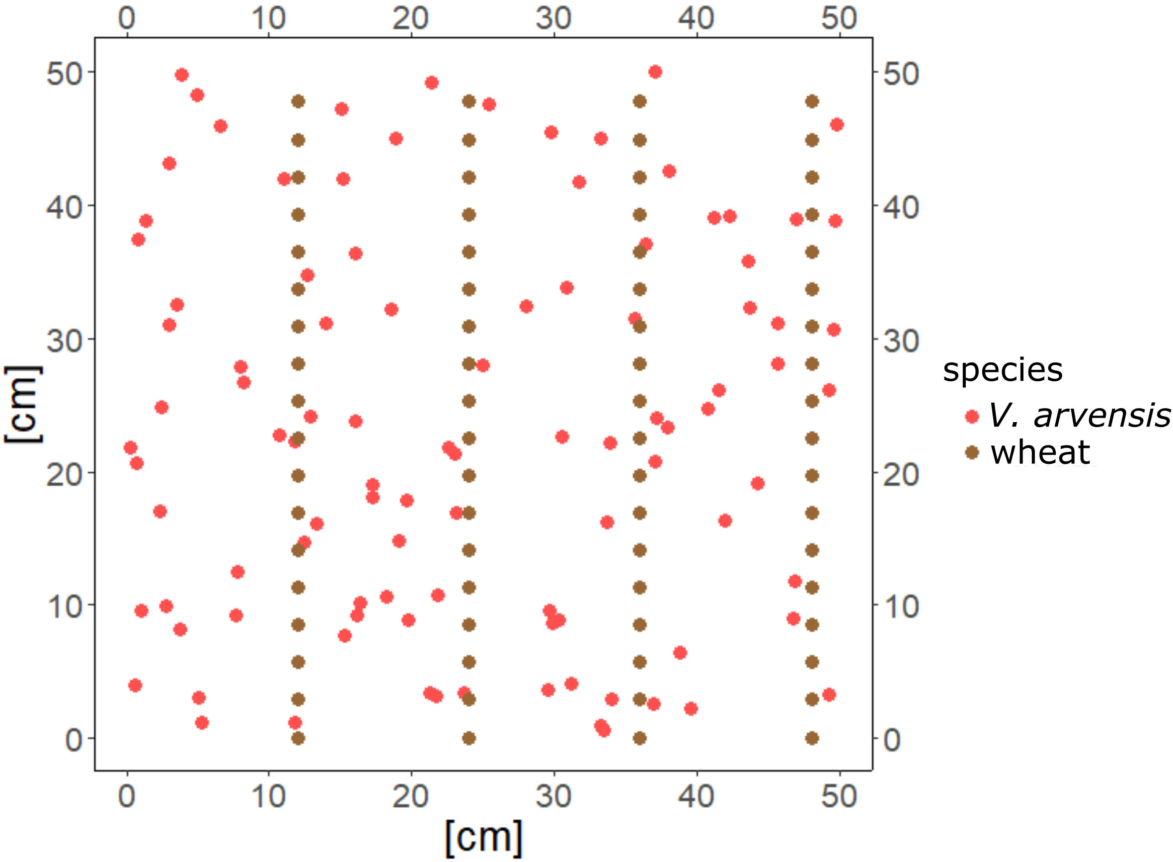
Figure 1 Example of a spatial configuration of crop weed plants.

2.1.2 Plant height growth

Notations for the following equations are given in Table 1. The growth of a single plant is modelled with a logistic growth equation (Equation 1). The corresponding analytical solution is given in Equation 2.

$\begin{array}{ll}\frac{dy}{dt}=r y-\alpha y^2& (1)\end{array}$

$\begin{array}{ll}y(t)=\frac{K\text{y}0}{\text{y}0-(y_o-K){\text{e}}^{-rt}} \text{with} K=\frac{r}{\alpha }& (2)\end{array}$

The notations are $y$: the plant height [cm], $r$: the growth rate [1/d], $\alpha$: retardation factor [1/cm], $K$: maximum height parameter [cm]. The logistic form was chosen, because it was shown to perform very well in diverse application of plant height growth (Jiang et al., 2020; Liao et al., 2023).

2.1.3 Crop weed interaction

The growth of individual plants, denoted with $i$ are coupled with the growth of neighboring plants $j$ (Equation 3).

$\begin{array}{ll}\frac{d{y}_i}{dt}=r_i{y}_i-y_i{\sum }_{j=1}^n{\alpha }_{ij}{y}_j& (3)\end{array}$

$\begin{array}{ll}A=\left(\begin{array}{cc}CC& WC\\ CW& WW\end{array}\right)& (4)\end{array}$

The coefficients $({\alpha }_{ij}$) are the elements of the community matrix A (Equation 4), which comprises the interactions between the plant species. This community matrix consists of four submatrices describing the interactions between crop pants ($CC$), the action of crop plants on weeds ($CW$), the action of weeds on the crop plants ($WC$), and the interaction between weeds ($WW$). In the model, the diagonal elements guarantee the retardation of growth of each individual plant. All other elements depend on the mutual distance $d_{ij}$ between plant $i$ and plant $j$.

$\begin{array}{ll}{\alpha }_{ij}=w_{ij}{e}^{-{\left(\frac{d_{ij}}{a}\right)}^{\gamma }}& (5)\end{array}$

The interaction terms ${\alpha }_{ij}$ (Equation 5) include the distance and the species-specific competitiveness. a describes the range of the effect. It is the distance at which the effect is reduced by $\frac{1}{e}$; $\gamma$ is a form factor. For $\gamma \ge 2$ threshold effects occur. The coefficient $w_{ij}$ measures the strength of competition between plants $i$ and $j$ and is specific for the type of interaction (crop-crop, crop-weed, weed-crop and weed-weed), i.e. the coefficient can take on only four values.

2.1.4 Emergence patterns

Whereas the growth of the crop plants is synchronous, weed emergence may occur over a longer period in cohorts. This is modelled by a delta distribution (Equation 6).

$\begin{array}{ll}\frac{d{y}_i}{dt}=\delta (t-t_i)y_{0i}+r_i{y}_i-y_i{\sum }_{j=1}^n{\alpha }_{ij}{y}_j& (6)\end{array}$

Here, t_i is the emergence time of weed $i$ and $y_{0i}$ is the initial value at time of emergence. The emergence time is the realization of a random variate for a given emergence pattern, which is modelled by the weighted sum (Equation 7) over a normal distributions truncated at zero (Equation 8).

$\begin{array}{ll}f(t)={\sum }_{j=1}^n{ɡ}_{i}h(t,{\sigma }_j,{\mu }_e)& (7)\end{array}$

$\begin{array}{ll}h(t,\sigma ,{\mu }_e)=\frac{2}{\sqrt{2\pi }\sigma }\exp \left(-\frac{{(x-{\mu }_e)}^2}{2{\sigma }^2}\right)/(1-\text{erf}\left(-\frac{\frac{{\mu }_e}{\sigma }}{\sqrt{2}}\right))& (8)\end{array}$

The ${ɡ}_i$ are weight factors normalized to 1. The delta distribution is approximated by a normal density function with a small value of ${\sigma }_t$ (Equation 9).

$\begin{array}{ll}\delta (t-t_i)\approx \frac{1}{\sqrt{2\pi }{\sigma }_t}\exp \left(-\frac{{(t-t_i)}^2}{2{\sigma }_t{}^2}\right)& (9)\end{array}$

2.1.5 Management

For many model applications in agricultural context weed control measures are essential. Therefore, weed control is taken into account by adding a further term to the differential equations for the weed describing the effect of a control measure on weed growth (Equation 10).

$\begin{array}{ll}{\mu }_c(t)=h\left(t-t_{app}\right)d_{max}{e}^{-\frac{(t-t_{app})}{\tau }} a(P_i)& (10)\end{array}$

The factor $h\left(t-t_{app}\right)$ is the Unitstep function with application time $t_{app}$. The parameter $d_{max}$ stands for maximum impairment. Besides damaging the weed, this model approach also allows a recovery following the damage with mean recovery time $\tau$ [d]. If $\tau$ is set to infinity, no recovery is possible. The index $i$ refers to individual weed plants, $P_i$ is the location and $a(P_i)$ ϵ (0,1) indicates, whether weed control has been performed at this location. Via the $a(P_i)$ term, spatial patterns of weed control are realized. In the case of multiple applications at times $t_i$ Equation 10 is generalized by

$\begin{array}{ll}{\mu }_c(t)={\sum }_{i=1}^{n}h(t-t_i)d_{\max i} e^{-\frac{(t-t_i)}{\tau }} a(P_i)& (11)\end{array}$

The full model for plant growth taken weed control into account is thus described by Equation 12.

$\begin{array}{ll}\frac{d{y}_i}{dt}=\delta (t-t_i)y_{0i}+r_i{y}_i-y_i{\sum }_{j=1}^n{w}_{ij}{e}^{-{\left(\frac{d_{ij}}{a}\right)}^{\gamma }}{y}_j-{\mu }_c(t)y_i& (12)\end{array}$

2.1.6 Parameterization

The resulting system of ordinary differential equations (ODEs) does not possess analytical solutions, i.e. solutions in closed form. For parameter estimation numerical solutions of the ODEs are therefore embedded into a standard least square estimation procedures using the routines NDSolve and NonlinearFit in Mathematica (Wolfram Research, Inc, 2021). As starting values for the growth curves described by the ODEs the mean of the parameters of the individual growth curves were used.

The data of a field experiment (see below) was used to stepwise parameterize the model. The growth of the individual plants is described by Equation 2. The parameters of the growth curve were estimated for every plant individually, in a first step. For the estimation of the competition coefficients, two suitable spatial configurations were chosen with four plants each. This approach did only allow to estimate the mutual competition parameters and the range parameter. Parameters for crop-crop and weed- weed interactions were fixed.

As a further method, simulation runs for the experimental situation were carried out using the parameters from the individual adjustments as a basis. In a second step, the interaction parameters were tuned by hand. To evaluate the effect of tuning, the plant height reached at the end of the experiment served as a comparison criterion between simulation and real data.

Table 1

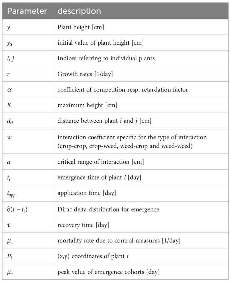
Table 1 Notations for the formulas used.

2.1.7 Modell application

Single-plant weed management enables farmers to precisely define which plant should be removed and which not. It is intuitively clear, that total removal of all weeds leads to maxium yields. However, in the following computer experiments, the question was addressed, if a coexistance of crop and weed is possible at tolerable yield losses. The parametrized model was applied to three scenarios with winter wheat. For all model runs 72 crop plants and up to 400 randomly distributed weed plants where used. Growth parameters are random following a uniform random distribution over the interval estimate +/- standard deviation derived from the statistical analysis of the experimental data (Table 2). This system of differential equations was solved numerically by the routine NDSolve in Mathematica. Emergence times of the weeds are random following the statistical distribution of emergence times as given by Equation 7.

Table 2

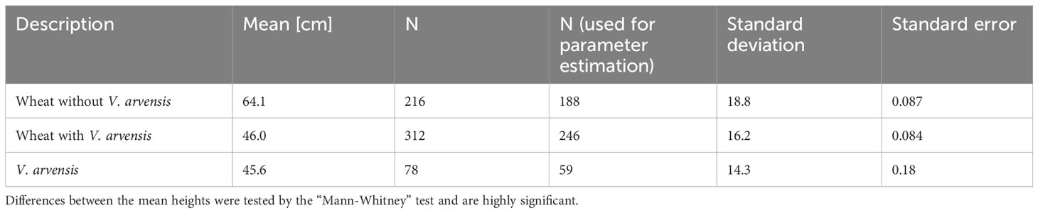
Table 2 Mean heights of wheat with and without competition from V.arvensis and mean height of V.arvensis.

The effect of multiple herbicide applications on the weed growth was analysed with the variation: one application (day 10), two applications (days 10 and 20), three applications (days 10, 20, and 35), and four applications (days 10, 20, 35, and 50) (Figure 2).

Figure 2

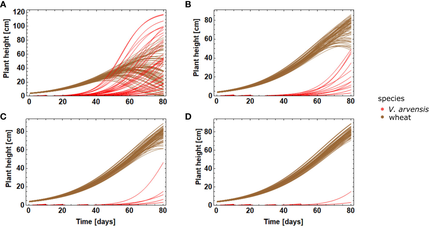
Figure 2 Effect of multiple applications on the growth dynamics of crop and weed (A) one application at t₁=10 d (B) two applications at $t_1$ = 10 d and $t_2$ = 20 d (C) three applications with at t₁ = 10 d, t₂= 20 d, and $t_3$ = 35 d (D) four applications at t₁ = 10 d, t₂ = 20 d, t₃ = 35 d, and $t_4$ = 50 d.

$\begin{array}{ll}a(x)=Min[ {\sum }_{i=1}^{\text{nrow}}\text{h}[x-({\text{Row}}_i-\text{d})](1-\text{h}[x-({\text{Row}}_i+\text{d})]),1]& (13)\end{array}$

In a second scenario, a weed strip control was performed. The width of the treated weed strips around the crop plants was varied between 0 cm and 10 cm. Weeds were removed within the strip and remained untouched outside (Equation 13). In addition to strip width, the weed density was varied as well (50, 75, 100, and 150 weed plants). Weed strip control is mediated via the term $a(P_i)$ in Equation 11, which takes the form where ${\text{Row}}_i$ denotes the x coordinate of row $i$ and the width of the treated strip with the row in the center.

In a third scenario the effect of the range of the competition effect in relation to weed density was analyzed.

2.2 Field experiment

In 2020 a field trial was conducted in Braunschweig, Germany. In this trial wheat was sown on October 29^th in 21 plots of size 1 m * 2 m. A quadrat measuring 36 cm * 36 cm was chosen for sampling at the edge of each plot, in order to be able to reach it easily for the measurements. The trial consisted of three variants: one variant with wheat and V. arvensis in 6 plots, one variant with wheat and V. arvensis, but some V. arvensis (plant number 4 and 6) plants were removed in the end of May in 7 plots, and the control with 8 plots only cropped with wheat. V. arvensis were planted on November 11^th at the seedling stage.

In each plot the height of all plants within the quadrat was measured every two weeks from the date of planting: 6 plants of V. arvensis and between 37 and 47 wheat plants. The measurement ended with the death or harvest of the plant. These data allow parameterizing growth curves for individual wheat plants as well as V. arvensis plants.

3 Results

3.1 Model parameters

3.1.1 Individual growth curves

For creating the growth curves the first eight wheat plants from every row were used and also all V. arvensis. Some plants showed a negative growth, so they died in the beginning. Others did not reach their maximum height yet and the capacity term would be fitted to infinity. We excluded plants with too small growth rate (r< 0.01), plants with a starting height (y0< 0), and plants with a maximum height larger than an upper limit of K > 180. This selection process resulted in 434 wheat plants and 59 V. arvensis plants (Table 2). Table 2 shows also the mean maximum heights measured. One can clearly see the difference in the growth heights. The competition from V. arvensis causes a significant reduction in height. Since the removal of V. arvensis in the end of May had no effect on wheat growth, the data sets concerning weed competition were combined.

Model parameters were estimated for each individual plant based on Equation 2. For the statistical evaluation only data from plants with normal growth behavior were considered which survived until harvesting and were thus suited for parameter estimation (Table 2). Figure 3 shows individual growth curves of four plants, crop and weed plants respectively. The model fit was satisfactory, as demonstrated by the plot of predicted vs. observed heights yielding a straight line with the slope of 1 (Figure 4). Comparing growth curves of wheat plants with and without competition through V. arvensis, the effect of weed competition is evident (Figure 5). Equation 2 was solved for three situations: wheat with V. arvensis, wheat without V. arvensis, and V. arvensis with wheat. Parameter estimates for all three solutions of Equation 2 are presented in Table 3 and Figure 6. The median height of wheat plants at harvest was 87.7 cm and 71.2 cm without competition and with competition respectively.

Figure 3

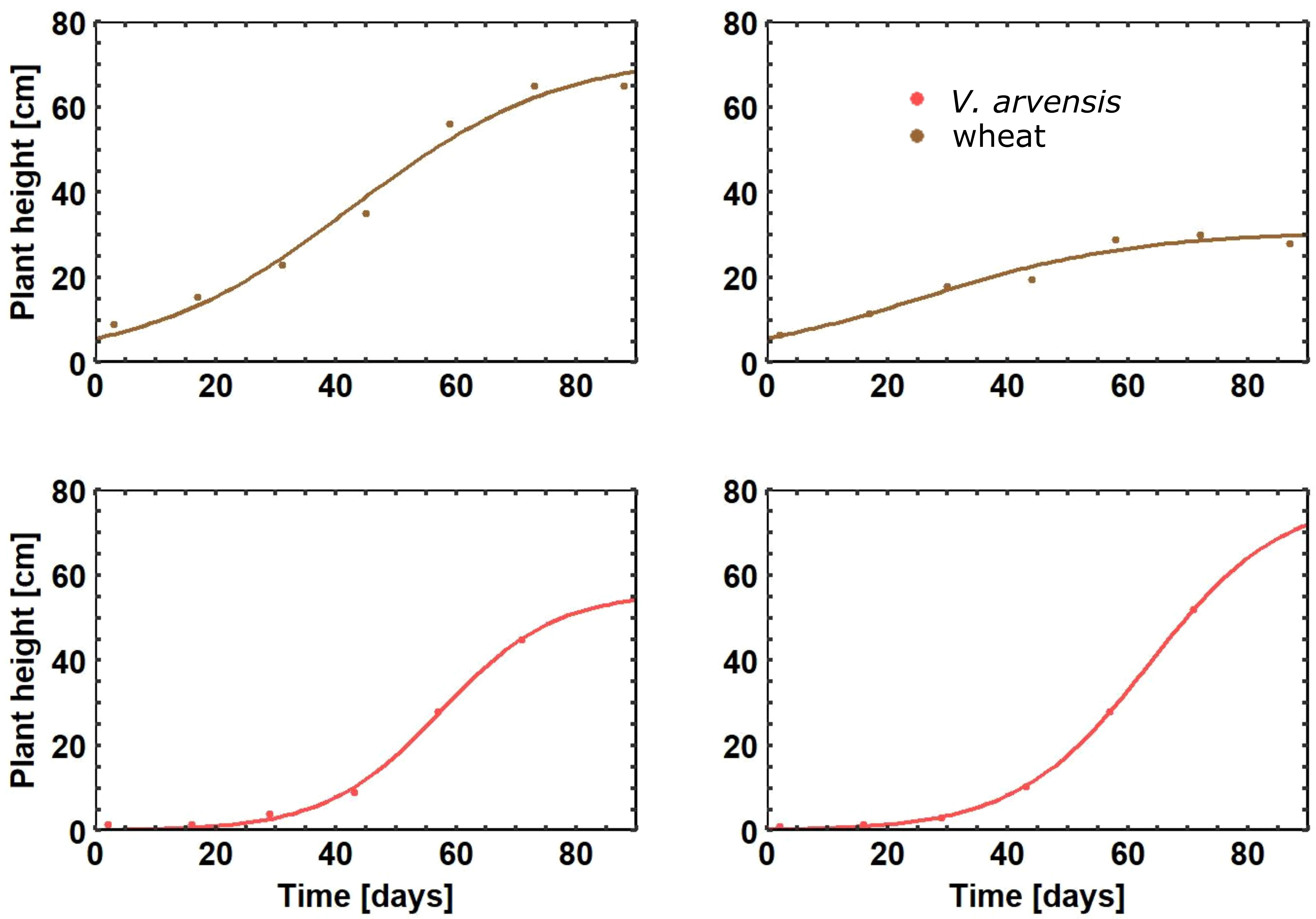
Figure 3 Selection of individual growth curves of wheat plants and of V. arvensis.

Figure 4

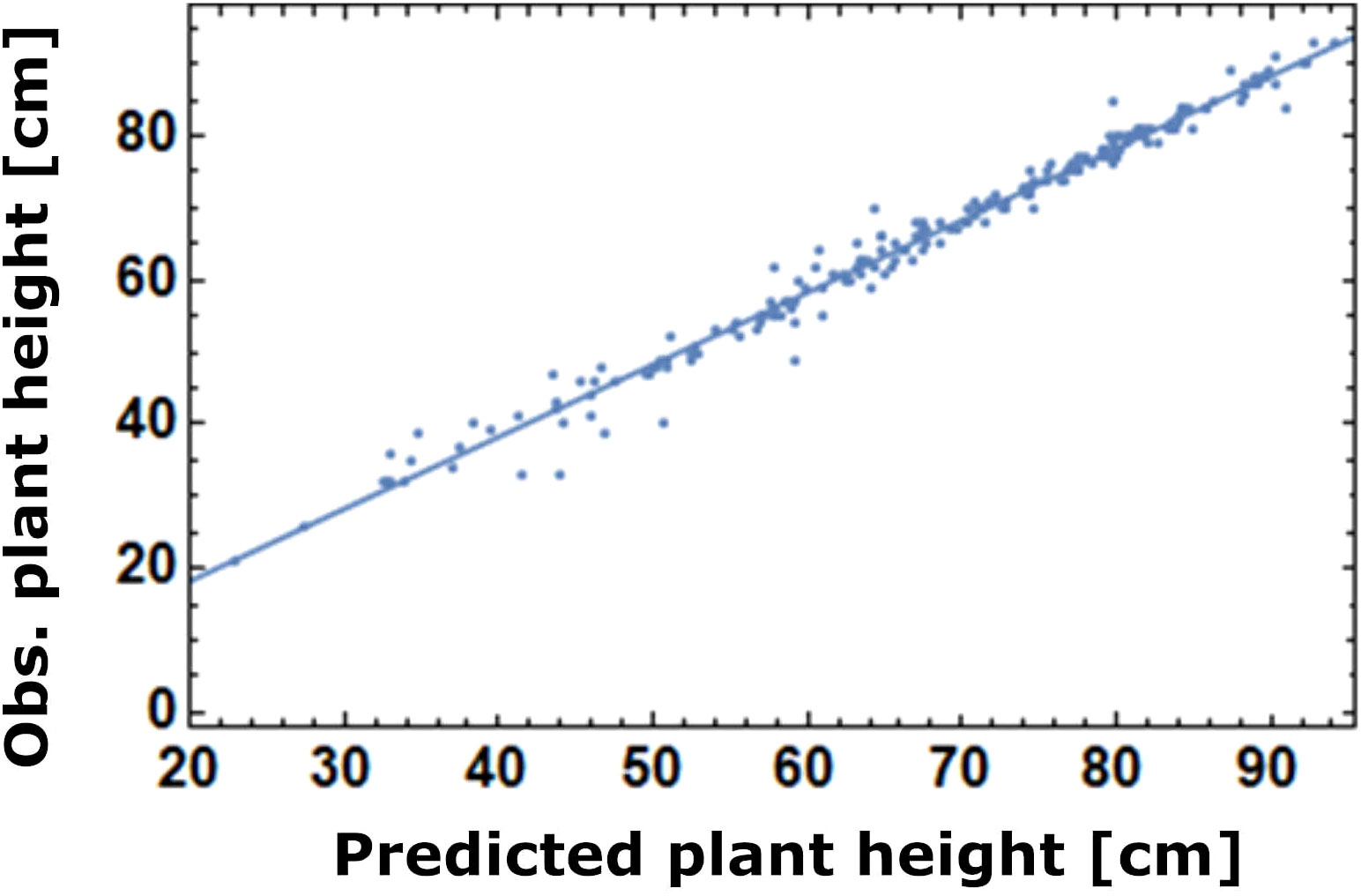
Figure 4 Plot of predicted vs observed heights at the end of the experiment. The confidence interval of the slope of the straight line is [0.970, 1.001] and of the confidence interval of the intercept is [-1.6, 0.4].

Figure 5

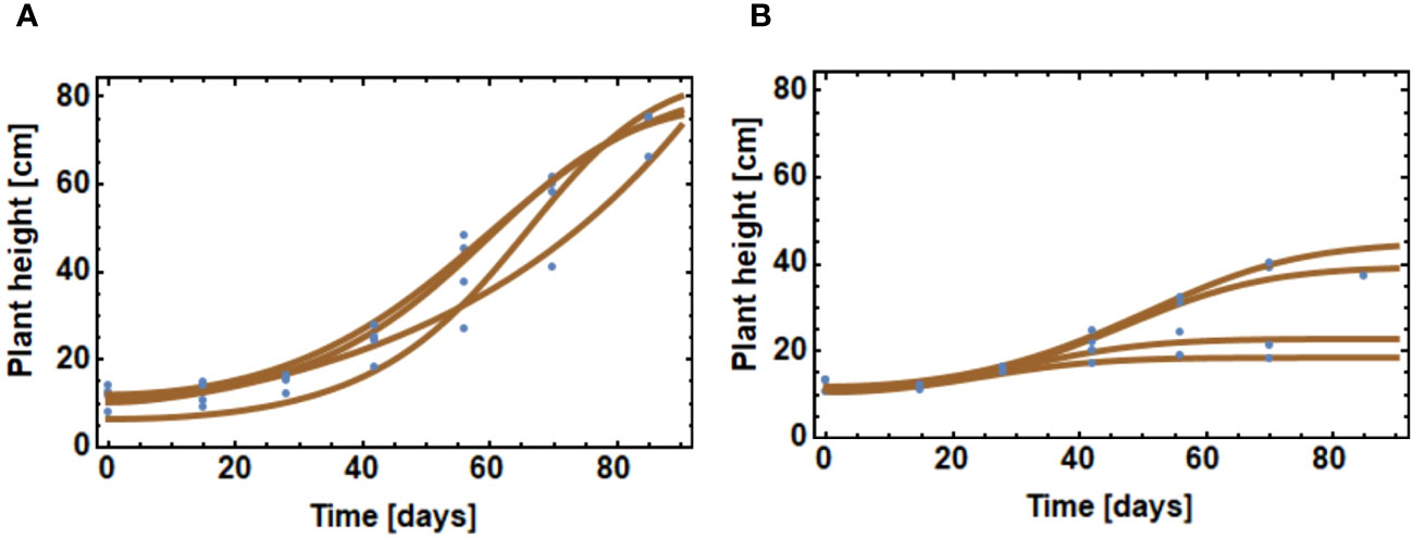
Figure 5 Sample of growth curves of crop plants (A) without competition (B) under competition.

Table 3

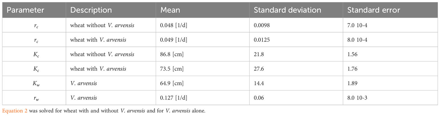
Table 3 Model parameters as derived from single plant analyses.

Figure 6

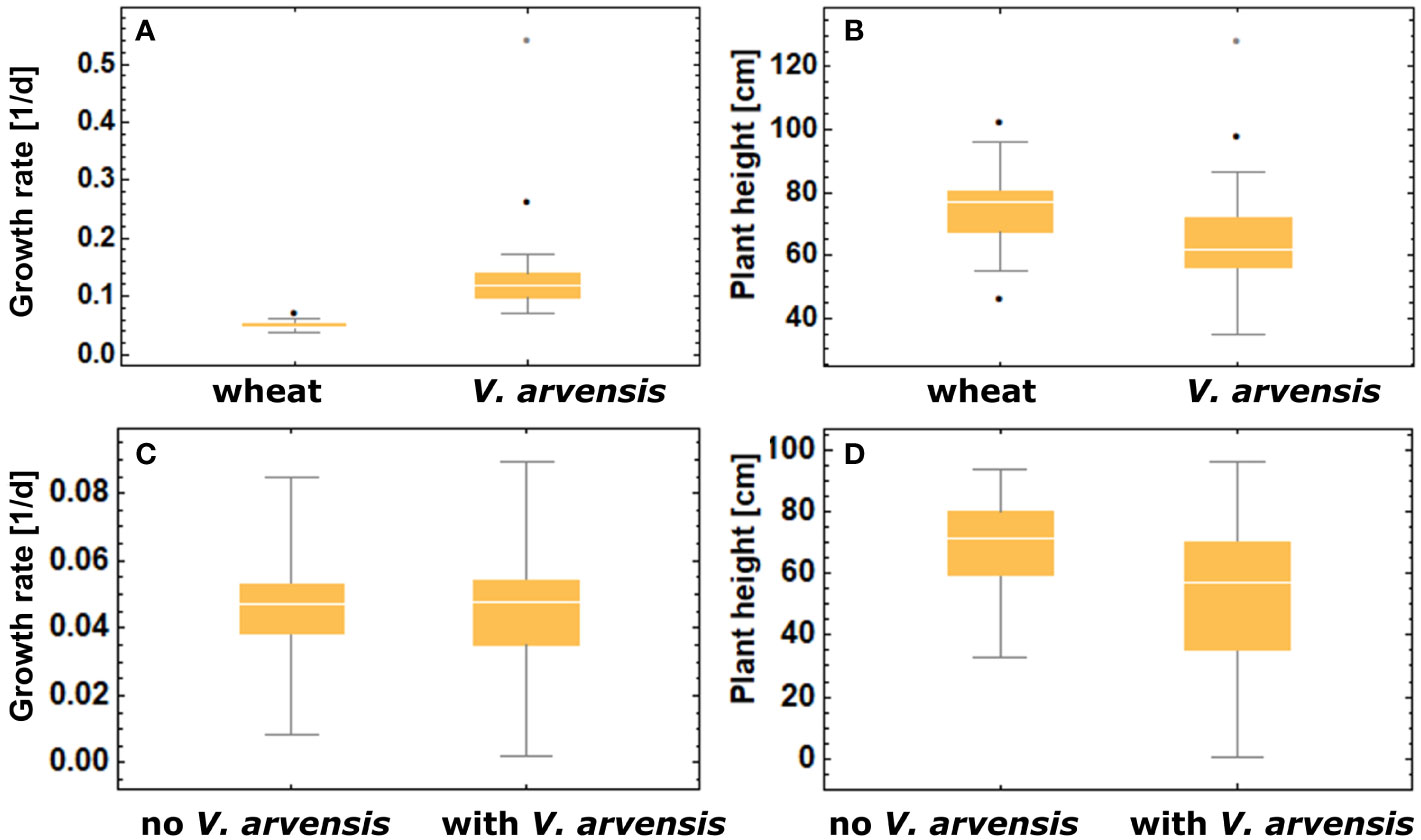
Figure 6 (A) Comparison of growth rate of all crop plants and weed plants (B) Comparison of maximum plant heights between crop and weeds (C) comparison of growth rates of crop plants grown with and without weed competition (D) comparison of maximum crop heights obtained with and without weed competition.

Looking at the boxplots of growth rates and maximal plant heights in Figure 6 reveals an interesting feature: competition does not affect the median value of crop growth rates (parameter $r$) but rather the maximum heights obtained (parameter $K$). These findings are confirmed by the “Mann‐Whitney” test. In addition, competition causes higher variability of growth parameters which also shows in Figure 4. In contrast to wheat, the growth rates of V. arvensis show a large variability. To evaluate the quality of the parametrization the trial setting was reconstructed with the model. The simulation output showed nearly identical results as the trials (Table 4) and thus the parametrization was a success.

Table 4

Table 4 Comparison between simulated and experimental data of the mean values for the maximum plant heights.

3.1.2 Competition coefficients

In order to model the growth of the plants together (Equation 3) the mean values of the single plants for the parameters $r$, $y_0$, and $k$(Table 3) were used as starting values for the ODEs. The competition coefficients $w_{ij}$ and the range parameter $a$ were estimated using two suitable spatial configurations chosen from the field experiment, since it was not possible to model all plants simultaneously in this step. These configurations consisted of one wheat plant and three plants V. arvensis with a maximum distance below 10 cm. Figure 7 shows the simultaneous fit of three weed plants and one crop plant taking into account the distance between individual plants. Therefore, the competition coefficients were combined to only one value. In this parameterization, the effect of weeds on crop and the effect of crop on weeds was assumed to be equal (Table 5).

Figure 7

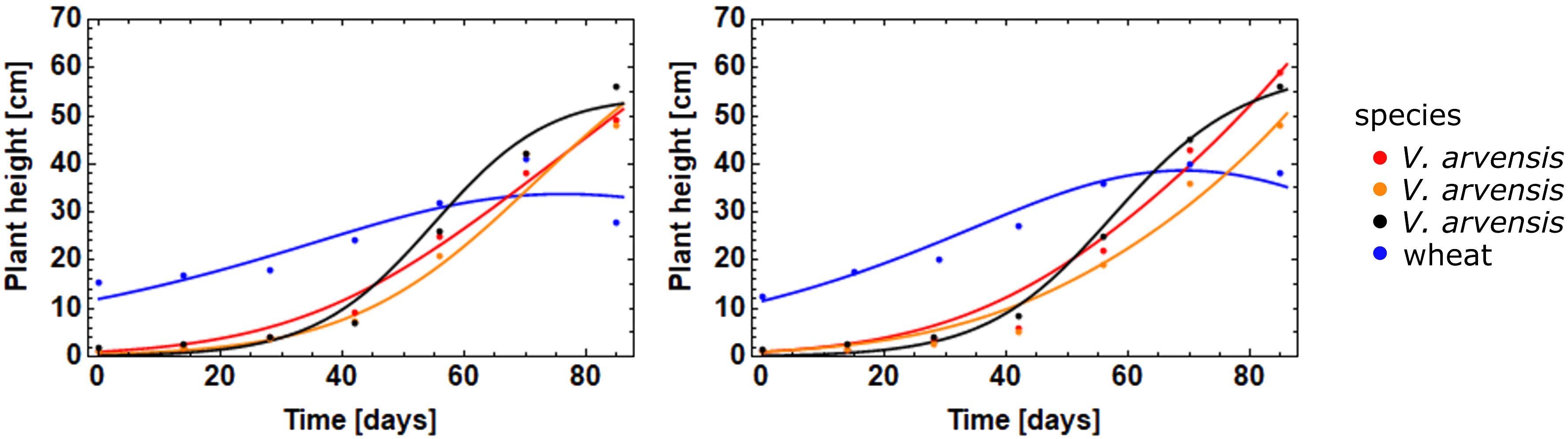
Figure 7 The simultaneous fit of growth curves of three weed plants and one crop plant (blue colour) taking into account mutual distances.

Table 5

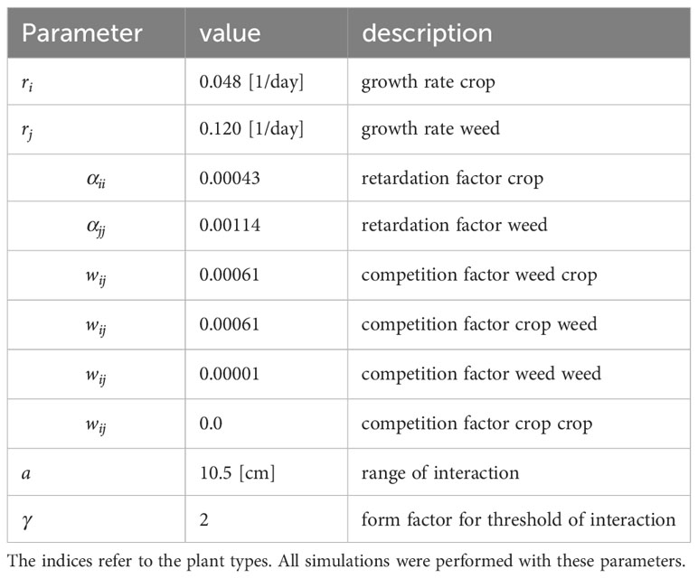
Table 5 Parameters of the complete model (Equation 3) as derived from single plant analyses, simultaneous estimation of competition coefficients, and by tuning.

3.2 Model applications

3.2.1 Mulitple herbicide applications

Crop varieties are bred to have a uniform emergence timing. Therefore, in our model all crop plants are made to emerge uniformly, while the emergence of V. arvensis follows patterns as described by Equations 7, 8. The following simulations are based on a typical emergence pattern for V. arvensis with several cohorts as shown in Figure 8. Controlling the first cohort only causes a large variability of wheat growth curves (Figure 2A). Wheat is overgrown by V. arvensis and only few wheat plants attain maximum height. An early herbicide application has no effect on later cohorts. However, since the first cohort is prevented from growing, the crop can develop well until the following cohorts appear. After two applications, the main cohorts are successfully suppressed and only few weeds of later cohorts are able to compete with wheat plants (Figure 2B). The variability of wheat growth curves is substantially reduced. After three uses respectively four uses, the competition is nearly eliminated (Figures 2C, D). The variability of the growth curves that still exists is due to the natural variability of the plants and is expressed in the variability of the parameters.

Figure 8

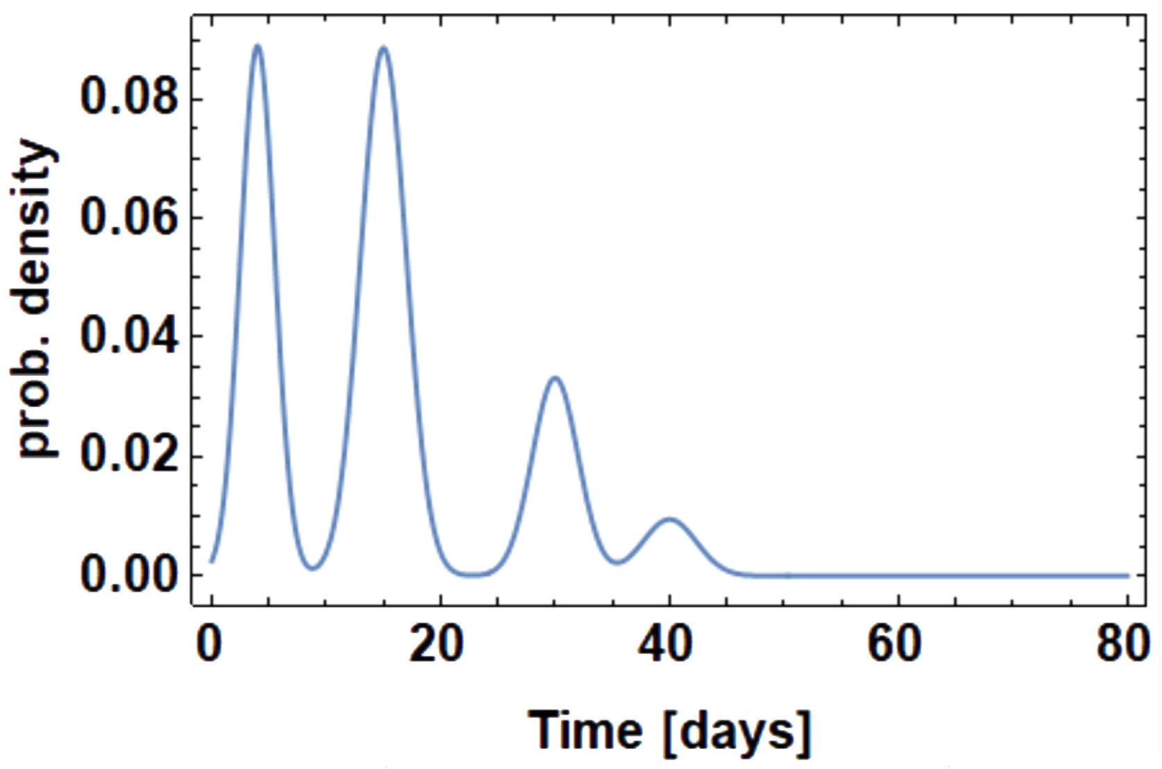
Figure 8 Probability density function for weed emergence with multiple cohorts used for the following simulations.

Figure 2A shows the severe effect of nearly uncontrolled competition of V. arvensis on wheat. Many weed plants grow very high and many of the crop plants suffer and cannot reach a reasonable height. The following Figures 2B–D show a growing effect of weed control. While the weeds are more and more restricted in growth, the crop gains in height and in homogeneity.

3.2.2 Weed strip control

Here, the effect of a buffer zone around the wheat-cropped rows was analysed. Weed control takes place only within a buffer zone. Figure 9 shows the effect of the width of the buffer zone on the height for different densities of V. arvensis. The width of the bufferstrip varied from from 0 cm to 9 cm around the wheat row. The stochastic elements of the simulation results in a variation of the resulting values for plant height. However, the (artificial) data points thus generated can be well fitted to a sigmoid curve of the form of (Equation 14).

Figure 9

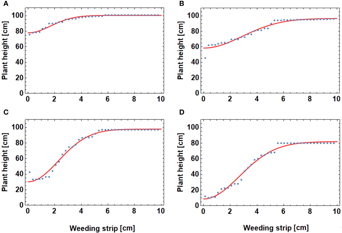
Figure 9 Plant height vs breadth of weeding strip for different values of weed densities [V. arvensis/m²]: (A) 50, (B) 200 (C) 300, and (D) 400.

$\begin{array}{ll}height(d)=y_0+(y_{max}-y_0)(1-\text{exp}(-(\frac{d}{d_{crit}}{)}^2)& (14)\end{array}$

Here, $d$ denotes the width of the strip, $d_{crit}$ a threshold value and $y_0$ is the remaining plant height for zero width, thus wheat height without weed control.

The results show that the effect of the weeding strip changes with its width and the weed density. When no weed control is conducted (weeding strip = 0 cm), the mean wheat height is the lowest. The maximum wheat height was reached with a weeding strip around 6 cm regardless of the overall weed density. The value of the maximum weed height on the other hand was decreasing with increasing weed density.

3.2.3 Influence of weed density on crop height

The model was used to investigate the repationship between crop height and weed density in dependence of the interaction range $a$ (Equation 5). Figure 10 shows weed density relationships for different values of the interaction range. The stochastic elements of the simulation runs show in the variation of the resulting crop height. However, the (artificial) data points thus generated can be well fitted to a sigmoid curve of the form of (Equation 15).

Figure 10

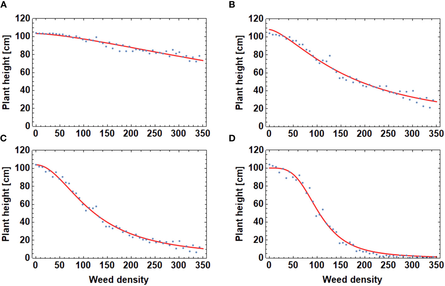
Figure 10 Crop height vs weed density for different values of the interaction range $a$: (A) $a$ = 2 cm (B) $a$ = 4 cm (C) $a$ = 7.5 cm, and (D) $a$ = 15.5 cm. Note that the height-density relationships are of sigmoid form.

$\begin{array}{ll}Y(w)=\frac{Y_{max}}{1+{(\frac{w}{thr})}^b} & (15)\end{array}$

where $w$ denote the weed density, $thr$ a threshold value and $b$ is a form factor.

The range of competition is specific to each weed species. Therefore, a sensitivity study of the height-density relationship with respect to the range parameter was performed. It turned out that this is a crucial parameter determining crop loss (Figure 10). With a low effect range of 2 cm the height is barely reduced even at high weed densities. With increasing range crop height is reduced in a non- linear way with a receding threshold. Below the threshold, the height is nearly unaffected. This effect has to be taken into account, if a system with several weed species is set up.

4 Discussion

We developed a model with the aim to simulate the plant height growth of single plants within a crop stand. Beside the growth, this model accounts for competition effects of single plants as well as management events. The realization of this concept implies model development, experiments, and parameter estimation as well as applications for weed control.

4.1 Model concept

Competition models used different approaches to simulate plant growth (Kropff, 1988; Wilson and Wright, 1990; Bagavathiannan et al., 2020; Colbach et al., 2021). Most simulation models for plant growth model an entire field or crop stand, which is an important tool for understanding the dynamics of crops and thus for weed management. Models simulating the growth of single plants within a crops stand are rare (but see Damgaard et al., 2002; Colbach et al., 2021). Here, coupled ordinary differential equations (ODE) were used as an easy way to simulate plant growth and competition. Already for a long time ODEs has been used for a small number of plants (Damgaard et al., 2002, i.e.). To our knowledge, this is the first time this method is applied to simulate hundreds of plants and their spatial interaction simultaneously. In the current form the number of plants is limited only by the machine running the simulation. The used ODEs can be easily modified to include germination cycles or management. The handling is relatively easy, which makes it a promising approach for single-plant modelling over large areas. Compared to the complex FlorSys environment (Colas et al., 2021) the ODE approach is easy to handle. The implementation of stochastic elements concerning growth rates, allocation of weed seeds and weed emergence mimics the high level of variation in nature. In addition, the efficacy of weed control is determined by a uniform random variable, similar to Renton et al. (2011). Especially the spatial aspect of the model is rarely adopted in models for the interaction weed-crop, which is only possible if single plants are addressed. The spatial arrangement of plants is the key for future management decisions, when plant-specific control measures are available.

4.2 Field trial and parameterisation

The core for parameterization are growth curves for individual plants, which resulted a wide range for the model parameters. Most importantly, the trial provided data for growth rates of wheat and V. arvensis under various conditions. The high number of plants in the field trial resulted in reliable values even though the variability within the data was very high. The observed plant height for V. arvensis are comparable to literature; most importantly the high variation in the results was observed bevor (Bachthaler et al., 1986). To estimate the competition parameters as well as the range parameter ODEs were used. The difficulties during parameterization of the ODEs were manifold: an effect of competition must exist and the solving algorithm must converge. The former was not very easy because of a relatively low number of weeds and thus a low level of interspecific competition, the latter is not easy because of the high variability in the plant growth data. Thus, the simultaneous parameter estimation using the differential equations turned out to be difficult. The experiment did only provide two situations/positions fitting to this requirements and which was not sufficient to estimate all parameters. The range parameter $a$ and one competition parameter $w_{ij}$ between crop and weed and vice versa could successfully be estimated. The approach of parameter tuning based on statistical comparison of the heights was very promising. Because the competition parameters depend on the current situation (Jornsgard et al., 1996), a parametrization for all wheat varieties, sites and conditions is not existent. Still, the parameter set presented here is one realistic possibility, which allows conducting computer experiments.

The current parameterization of the model shows reasonable results: The growth curves of wheat and V. arvensis in the simulations are comparable to the growth curves of the experiment with the corresponding trial conditions (Figures 2, 5). Still, for following trials or attempts for parametrization there should be more weedy situations, to facilitate the convergence of the solving algorithm for the ODE.

4.3 Model applications

The first model application simulated the growth of wheat and V. arvensis together under varying frequencies of weed control. The interaction between the plants and the variability of the plant height without weed control (Figure 2A) is severe and steadily decreasing with increasing intensity of weed control. Therefore, the parametrisation of the simulation model was plausible. Without weed control the mean plant height of wheat decreases and the variability of the growth increases dramatically. This corresponds with literature that reports decreasing mean plant height of wheat (Oad et al., 2006) and decreasing yield (Sarita et al., 2022). While the literature relies on mean values, the simulation additionally can decompose these mean values to single specific plants at specific positions. Thus, management decisions for individual plants could be made upon their specific growth.

The second model application covered a weeding strip around wheat with differing width and four levels of weed infestation. The density of V. arvensis had the most severe effect with narrow weeding strips: without weeding or with only small extend of weeding on the field and high weed density the plant height of wheat was reduced severely. When weeds on the entire area are managed, the wheat plant height reaches a maximum. However, the simulation provides a very fine grained picture on the level of weed management resp. the width of the weeding strip. The higher the weed density the steeper the curve of the wheat plant height, indicating that wheat can tolerate V. arvensis plants in a relatively high number, as long as they grow not very close to the crop. This effect is, at least experimentally, already used for intercropping wild plants in maize (Redwitz et al., 2019). The simulation indicates that weeding strips might be an option for weed management in cereal crops as well when the management tools are sufficiently precise.

The third model application gives insights on the range effect. The results show a strong effect off the range parameter on the wheat height as soon as the weed density is above a threshold. When the weed density is below 50 plants/m², the effect is neglectable. When the weed density is above that threshold the effect for small values of the range parameter stays small (Figure 10A). With a growing range parameter, its effect on wheat height gets stronger and stronger (Figures 10B–D). For the parameter as part of the simulation model this shows a high sensitivity of the results to this parameter. Therefore, care must be taken choosing the specific value for a parameterization. On a biological level, this provides insights on the effect of weeds with different phenotypes. The example weed V. arvensis is a relatively small species. Other species like Chenopodium album or Cirsium arvensis both growing taller and taking a lot of room (Eslami and Ward, 2021) would have a much higher range parameter than V. arvensis. Thus, simulations with these species would result in a lower wheat plant height.

The current parametrisation does not cover the potential of the model to its full extent. In further trials, more complex growing situations should be established to allow more precise parameter estimation. The model itself can be extended to multiple species. This includes weeds, but other crops as well. To do this mainly the community matrix A (Equation 4) needs to be extended to cover the additional interactions.

For the application of the model, it will be most interesting to couple the simulation of plant growth with other plant traits beyond competition. If the model is extended to include the dynamics of the seedbank, longer periods can be simulated. Furthermore, other important aspects to consider in weed management like technical feasibility for harvest, storage and propagation might be included. Then the model could serve as a tool to plan the management of floral traits resp. ecosystem services in plant protection context and may play a role in solving the sharing or sparing debate for biodiversity conservation.

5 Conclusion

Spatial competition models for a large number of individual plants in form of systems of coupled nonlinear differential equations of a simple structure are capable of capturing the dynamics of the competition situation between weeds and crop plants. Once reasonable model parameters are obtained by experimental studies, the model is capable of evaluating spatially high resolved precision weed management. For a parameter set derived from an experimental basis involving wheat and the weed V. arvensis the simulations show that.

i) removal of weeds near the crop being grown is an option both for the reduction of weeding effort (chemical or mechanical) and maintenance of biodiversity.

ii) the relation between the neighbourhood distance for removal and plant height is a nonlinear threshold function with respect to the number of weeds emerged.

iii) weed emergence patterns may necessitate multiple applications.

iv) plant height reduction is both dependent on the number of weeds emerged and their range of competition.

The generic structure of the model allows the inclusion of additional weed species. The model is therefore a powerful tool for the improvement in weed control both by the assessment of management options in general and as decision support for adaptive weed control.

Especially decision support systems (DSS) for site-specific weed management are scarce but approaches combining weed mapping and DSS for site-specific decision support exist (Somerville et al., 2019; Gerhards et al., 2022). Up to now there is no DSS that supports based on single plants differentiated decisions, which is necessary to use the abilities of weed control technologies of the current generation to its full extend. The core of a single-plant based DSS would be a model representing the growth of all plants in a certain neighbourhood at the same time, such as the model proposed.

Data availability statement

The raw data supporting the conclusions of this article will be made available by the authors, without undue reservation.

Author contributions

CvR: Conceptualization, Data curation, Formal analysis, Investigation, Methodology, Project administration, Software, Writing – original draft, Writing – review & editing. JL: Data curation, Formal analysis, Methodology, Software, Validation, Visualization, Writing – review & editing. OR: Conceptualization, Formal analysis, Investigation, Methodology, Software, Visualization, Writing – original draft, Writing – review & editing.

Funding

The author(s) declare that no financial support was received for the research, authorship, and/or publication of this article.

Acknowledgments

We thank B. Tankir and N. Ritter for their intense work on the field trial. Without precise measuring in the real world, our simulation model cannot work.

Conflict of interest

The authors declare that the research was conducted in the absence of any commercial or financial relationships that could be construed as a potential conflict of interest.

Publisher’s note

All claims expressed in this article are solely those of the authors and do not necessarily represent those of their affiliated organizations, or those of the publisher, the editors and the reviewers. Any product that may be evaluated in this article, or claim that may be made by its manufacturer, is not guaranteed or endorsed by the publisher.

References

Anul Haq M. (2022). CNN based automated weed detection system using UAV imagery. Comput. Syst. Sci. Eng. 42, 837–849. doi: 10.32604/csse.2022.023016

CrossRef Full Text | Google Scholar

Bachthaler G., Neuner F., Kees H. (1986). Development of the field pansy (Viola arvensis Murr.) in dependance of soil conditions and agricultural management. Nachrichtenblatt Des Deutschen Pflanzenschutzdienstes 38(3), 33-41. Available at: https://www.openagrar.de/receive/openagrar_mods_00068864

Google Scholar

Bagavathiannan M. V., Beckie H. J., Chantre G. R., Gonzalez-Andujar J. L., Leon R. G., Neve P., et al. (2020). Simulation models on the ecology and management of arable weeds: structure, quantitative insights, and applications. Agronomy 10, 1611. doi: 10.3390/agronomy10101611

CrossRef Full Text | Google Scholar

Colas F., Gauchi J.-P., Villerd J., Colbach N. (2021). Simplifying a complex computer model: Sensitivity analysis and metamodelling of an 3D individual-based crop-weed canopy model. Ecol. Model. 454, 109607. doi: 10.1016/j.ecolmodel.2021.109607

CrossRef Full Text | Google Scholar

Colbach N., Colas F., Cordeau S., Maillot T., Queyrel W., Villerd J., et al. (2021). The FLORSYS crop-weed canopy model, a tool to investigate and promote agroecological weed management. Field Crops Res. 261, 108006. doi: 10.1016/j.fcr.2020.108006

CrossRef Full Text | Google Scholar

Confalonieri R., Bregaglio S., Rosenmund A. S., Acutis M., Savin I. (2011). A model for simulating the height of rice plants. Eur. J. Agron. 34, 20–25. doi: 10.1016/j.eja.2010.09.003

CrossRef Full Text | Google Scholar

Damgaard C., Weiner J., Nagashima H. (2002). Modelling individual growth and competition in plant populations: growth curves of Chenopodium album at two densities. J. Ecol. 90, 666–671. doi: 10.1046/j.1365-2745.2002.00700.x

CrossRef Full Text | Google Scholar

Eslami S. V., Ward S. (2021). “Chapter 5 - Chenopodium album and Chenopodium murale,” in Biology and Management of Problematic Crop Weed Species. Ed. Chauhan B. S. (London, United Kingdom: Academic Press), 89–112.

Google Scholar

Fang S.-L., Kuo Y.-H., Kang L, Chen C.-C., Hsieh C.-Y., Yao M.-H., et al. (2022). Using sigmoid growth models to simulate greenhouse tomato growth and development. Horticulturae 8, 1021. doi: 10.3390/horticulturae8111021

CrossRef Full Text | Google Scholar

Fernández-Quintanilla C., Dorado J., Andújar D., Peña J. M. (2020). “Site-specific based models,” in Decision Support Systems for Weed Management. Eds. Chantre G. R., González-Andújar J. L. (Cham: Springer International Publishing), 143–157.

Google Scholar

Gerhards R., Andújar Sanchez D., Hamouz P., Peteinatos G. G., Christensen S., Fernandez-Quintanilla C. (2022). Advances in site-specific weed management in agriculture—a review. Weed Res. 62, 123–133. doi: 10.1111/wre.12526

CrossRef Full Text | Google Scholar

Gerowitt B., Heitefuss R. (1990). Weed economic thresholds in cereals in the Federal Republic of Germany. Crop Prot. 9, 323–331. doi: 10.1016/0261-2194(90)90001-N

CrossRef Full Text | Google Scholar

Hamouz P., Hamouzová K., Holec J., Tyšer L. (2014). Impact of site-specific weed management in winter crops on weed populations. Plant Soil Environ. 60, 518–524. doi: 10.17221/636/2014-pse

CrossRef Full Text | Google Scholar

Huang H., Deng J., Lan Y., Yang A., Deng X., Wen S., et al. (2018). Accurate weed mapping and prescription map generation based on fully convolutional networks using UAV imagery. Sensors 18, 3299. doi: 10.3390/s18103299

PubMed Abstract | CrossRef Full Text | Google Scholar

Jiang T., Liu J., Gao Y., Sun Z., Chen S., Yao N., et al. (2020). Simulation of plant height of winter wheat under soil Water stress using modified growth functions. Agric. Water Manage. 232, 106066. doi: 10.1016/j.agwat.2020.106066

CrossRef Full Text | Google Scholar

Jornsgard B., Rasmussen K., Hill J., Christiansen J. L. (1996). Influence of nitrogen on competition between cereals and their natural weed populations. Weed Res. 36, 461–470. doi: 10.1111/j.1365-3180.1996.tb01675.x

CrossRef Full Text | Google Scholar

Keller M., Gutjahr C., Möhring J., Weis M., Sökefeld M., Gerhards R. (2014). Estimating economic thresholds for site-specific weed control using manual weed counts and sensor technology: An example based on three winter wheat trials. Pest Manage. Sci. 70, 200–211. doi: 10.1002/ps.3545

CrossRef Full Text | Google Scholar

Kropff M. J. (1988). Modelling the effects of weeds on crop production. Weed Res. 28, 465–471. doi: 10.1111/j.1365-3180.1988.tb00829.x

CrossRef Full Text | Google Scholar

Liao Z., Zheng J., Fan J., Pei S., Dai Y., Zhang F., et al. (2023). Novel models for simulating maize growth based on thermal time and photothermal units: Applications under various mulching practices. J. Integr. Agric. 22, 1381–1395. doi: 10.1016/j.jia.2022.08.018

CrossRef Full Text | Google Scholar

Liu F., Liu Y., Su L., Tao W., Wang Q., Deng M. (2022). Integrated growth model of typical crops in China with regional parameters. Water 14, 1139. doi: 10.3390/w14071139

CrossRef Full Text | Google Scholar

Marshall E. J. P., Brown V. K., Boatman N. D., Lutman P. J. W., Squire G. R., Ward L. K. (2003). The role of weeds in supporting biological diversity within crop fields*. Weed Res. 43, 77–89. doi: 10.1046/j.1365-3180.2003.00326.x

CrossRef Full Text | Google Scholar

Niemann P. (1981). SChadschwellen bei der Unkrautbekämpfung Vol. 257 (Münster-Hiltrup: Landwirtschaftsverlag GmbH). Angewandte Wissenschaft.

Google Scholar

Oad F. C., Siddiqui M. H., Buriro U. A. (2006). Growth and yield losses in wheat due to different weed densities. Asian J. Plant Sci. 6, 173–176. doi: 10.3923/ajps.2007.173.176

CrossRef Full Text | Google Scholar

Petit S., Boursault A., Guilloux M., Munier-Jolain N., Reboud X. (2011). Weeds in agricultural landscapes. A review. Agron. Sustain. Dev. 31, 309–317. doi: 10.1051/agro/2010020

CrossRef Full Text | Google Scholar

Redwitz C., Glemnitz M., Hoffmann J., Brose R., Verch G., Barkusky D., et al. (2019). Microsegregation in maize cropping—a chance to improve farmland biodiversity. Gesunde Pflanzen 71, 87–102. doi: 10.1007/s10343-019-00457-7

CrossRef Full Text | Google Scholar

Renton M., Diggle A., Manalil S., Powles S. (2011). Does cutting herbicide rates threaten the sustainability of weed management in cropping systems? J. Theor. Biol. 283, 14–27. doi: 10.1016/j.jtbi.2011.05.010

PubMed Abstract | CrossRef Full Text | Google Scholar

Sarita, Singh I., Mehriya M. L., Samota M. K. (2022). A study of wheat-weed response and economical analysis to fertilization and post-emergence herbicides under arid climatic conditions. Front. Agron 4. doi: 10.3389/fagro.2022.914091

PubMed Abstract | CrossRef Full Text | Google Scholar

Somerville G. J., Jørgensen R. N., Bojer P., Rydahl P., Dyrmann M., Andersen P., et al. (2019). “Marrying futuristic weed mapping with current herbicide sprayer capacities,” in Precision agriculture’19. Ed. Stafford J. V. (Wageningen: Wageningen Academic Publishers), 231–237. 12th European Conference on Precision Agriculture, Montpellier, France, 08-11 07. doi: 10.3920/978-90-8686-888-9_28

CrossRef Full Text | Google Scholar

Storkey J., Westbury D. B. (2007). Managing arable weeds for biodiversity. Pest Manage. Sci. 63, 517–523. doi: 10.1002/ps.1375

CrossRef Full Text | Google Scholar

Wilson B. J., Wright K. J. (1990). Predicting the growth and competitive effects of annual weeds in wheat. Weed Res. 30, 201–211. doi: 10.1111/j.1365-3180.1990.tb01704.x

CrossRef Full Text | Google Scholar

Wolfram Research, Inc (2021). Mathematica (Champaign, Illinois: Wolfram Research, Inc).

Google Scholar