Ray tracing model for long-range acoustic vortex wave propagation underwater

The use of vortex waves in multiple environments is of increasing interest for numerous applications including underwater acoustic communications, particle manipulations, and sonothrombolysis. Finite element methods are limited in the range for which the propagation of these vortex beams may be simulated. On the other hand, ray tracing programs simulate well over long ranges, though are generally limited in their ability to resolve the features of a propagating vortex. Methods for overcoming these difficulties in simulating the long-range propagation of such waves in inhomogeneous environments have been developed and employed, though their specific implementation has not been thoroughly discussed. This manuscript provides the methods by which existing ray tracing programs may be used to approximate the long-range propagation of acoustic vortex beams in complex environments.

1 Introduction

Vortex waves have garnered significant interest in both the optics and acoustics communities (Hefner and Marston, 1999; Zhang and Marston, 2011). Acoustic implementations of vortex beams have found use for numerous applications in medical treatments (Guo et al., 2022; Zhang et al., 2023), acoustic communications (Shi et al., 2017), particle manipulation (Fan and Zhang, 2019; Lo et al., 2021; Zhang et al., 2022), and other fields (Guo et al., 2022b). As further applications are explored, robust and efficient simulation tools are required. Finite element methods (FEM) are a powerful tool for performing high-resolution simulations of complex phenomena; however, they are severely limited in their ability to compute long-range propagation. Due to mesh size requirements, computational cost increases exponentially with range, often making long-range simulations impossible. Ray tracing programs, on the other hand, are readily available for many applications and are efficient over long ranges, especially when compared with FEM. These programs are not always equipped with the tools necessary to handle the helical ray paths of an acoustic vortex. Two-dimensional (2D) ray tracing codes cannot on their own resolve features which are inherently 3-dimensional (3D), and 3D ray tracing algorithms (including Nx2D iterations of 3D ray tracing) may not be equipped to account for the orbital angular momentum of a propagating vortex. This manuscript provides an explicit handling of the methods which were first published in (Fan et al., 2019) and presented in (Zou et al., 2020a) by which 2-dimensional ray tracing models were employed to calculate vortex propagation in complex environments and can resolve the helical wave pattern over long-range simulations. These methods use ray tracing methods in each of the transducers propagating planes to then extrapolate to calculate the behavior of the whole field. This accounts for the restorative forces the orbital angular momentum exerts on the streamlines and allows the user to examine slices of the 3D space. This work is based on the BELLHOP ray tracing algorithm (Jensen et al., 1995), though any well-established and tested ray tracing code should achieve similar results.

2 Background

Ray tracing presumes that the energy emitted from an acoustic source is divided amongst a number of discrete beams which traverse the environment. The underwater acoustic environment, specifically, is inhomogeneous due to variations in pressure, salinity and temperature within a water column. As a result, the traversing beams refract according to Snell’s law. Due to reflections at the boundaries and refraction within the bulk, only a subset of the rays will connect a given source and receiver. These rays are called eigenrays. Summing the contributions from the eigenrays gives a complex pressure which is typically used by BELLHOP to calculate transmission loss. The principal limitation of ray tracing is that it is generally well adapted to higher frequency where the wavelength is short compared to the length scales of the environment. With longer wavelengths, the width of the effective ray becomes larger. In the limit where wavelength is on the order of the length scale of the environment, the propagating energy can no longer be effectively discretized among individual rays. For a more rigorous handling of acoustic ray tracing and the BELLHOP model, the reader should refer to (Jensen et al., 1995).

Bessel type vortex waves are a subset of non-diffracting beams whose propagating field is characterized by a rotating helical pattern. The amount of rotation inherent in the propagating vortex is given by the topological charge l. The resulting phase change over the helix is given by $2\pi l$, where l is typically given as an integer. For an array consisting of multiple concentric rings of transducers, Eq. 1 gives the phase relationships as determined by the Bessel function.

$\theta =J_0\left(kr\right)e^{i\phi l}(1)$

Here, k represents the in-plane wavenumber and the source is located at the polar coordinates (r, φ). The non-diffracting characteristic of a Bessel beam is limited by its aperture (Durnin et al., 1987), therefore, these defining characteristics do not apply over long ranges, especially in inhomogeneous environments. While several methods have been presented to form vortex waves, this model relies on arrays like those presented in Shi et al. (Shi et al., 2017) and Kelly and Shi (Kelly and Shi, 2023), which are comprised of concentric rings of N transducers (Cain and Umemura, 1986; Umemura and Cain, 1989). An array configuration consisting of 3 concentric rings of radii 5, 10, and 15 wavelengths with phases determined using Eq. 1 was used with a frequency of 15 kHz and topological charge l = +1 to generate the figures presented in this work unless otherwise stated. A pictorial representation of this array is presented in the Supplementary Material.

The model presented below was first introduced in (Fan et al., 2019) and explored further in Kelly and Shi (Kelly and Shi, 2023). It relies on the assumption that each of the transducers in the array can be approximated as an individual point source, which allows for visualization of vortex propagation either as range vs. depth (perpendicular to the vortex) or the wavefront plane (parallel to the vortex). As validation of these methods, the BELLHOP solution is compared to an analytical solution calculated using Eq. 2 which represents spherical spreading in a homogeneous free space environment.

$p\left(r\right)=\sum \frac{1}{r_n}{e}^{i\left(k{r}_n+{\theta }_n\right)}(2)$

3 Range vs. depth plots

Range vs. depth plots are perhaps the simpler of the two cases. To simulate the propagating vortex, each transducer in the array is simulated as its own individual point source within the given environment using the coherent transmission loss function of BELLHOP. The output to this function is a.shd file that contains complex pressure for the points of interest, which were designated in the.env file. With the individual transducers simulated at the proper depths, and by applying the appropriate phase shifts as calculated using Eq. 1 and depicted in Supplementary Figure S1, coherently summing these pressure fields yields the desired result. Figure 1 shows the 2D range vs. depth normalized pressure field for the same array in an infinite homogenous environment solved analytically and using BELLHOP. The central singularity represents the center of the vortex, and its propagation can be followed by tracing this singularity. These methods do not account for the fact that the transducers in the array are out-of-plane relative to each other. Over longer ranges (range is much greater than the array radius such that the difference between the propagation distances for center source and that of out-of-plane source is negligible), this assumption is valid; however, at shorter ranges this can lead to some discrepancies between the BELLHOP and analytical calculations as is seen in Figure 1. This difference highlights an important note that in order to fully understand the behavior of the vortex, it is important to use these plots alongside a corresponding wavefront plane plot. This is especially true in more complex environments where multi-path propagation and the complex side lobe structure can make the range vs. depth plots alone difficult to interpret. Additionally, it is important to note that because BELLHOP is designed to compute transmission loss, the acoustic pressure at the source is irrelevant, and is therefore normalized. For accurate predictions of real or complex pressure, this must be adjusted by the user. Environmental uncertainty is likely to impact the accuracy of the complex pressure calculations, so it is generally acceptable to use these normalized results as a method of determining whether the vortex wave will survive under the simulated conditions.

FIGURE 1

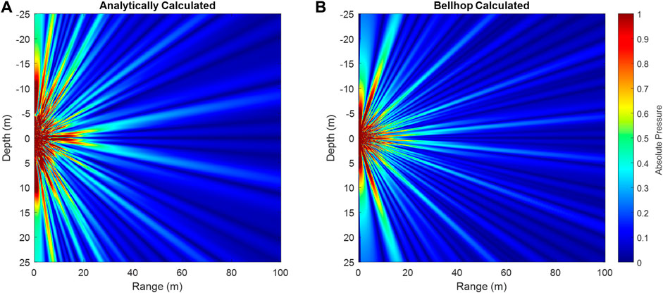
FIGURE 1. Analytically (A) and BELLHOP (B) calculated propagation of a 15 kHz vortex wave in a homogeneous environment. The analytically calculated plot results in a clearer interference pattern, especially near the array, though the central singularity is clearly visible in both plots and the general structure of the side lobes is similar.

4 Wavefront plane plots

The wavefront plane is somewhat more difficult. At its core, the methodology is similar. Modelling the wavefront plane requires the proper handling of position and phase for each of the transducers in the array as determined using Equation 1. The amplitude and phase changes between points in the wavefront plane are taken to be caused by the difference in propagation distance between the transducer and those points. To calculate this, we project the appropriate pressure values from the ranges of interest in the range plane onto the wavefront plane. We then apply the appropriate phase shift for the transducer being calculated, and sum coherently over all transducers to reconstruct the vortex. The spatial resolution required to faithfully reconstruct the vortex is relatively high ((Fan et al., 2019) used 10 samples per wavelength, though 3 samples per wavelength is generally sufficient). Figure 2 contains a pictorial representation of this approach. The black arrow represents the straight-line distance which is perpendicular to both the transmitter and receiver planes. The red arrow represents the distance from the transducer being simulated to the point in the plane which is being calculated. To determine the pressure value at these points, the Bellhop simulation should include receivers at all r’ locations required to reconstruct the wavefront plane.

FIGURE 2

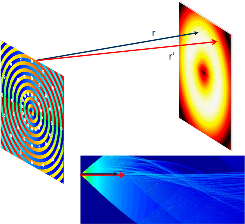
FIGURE 2. A schematic diagram depicting how pressure is translated from the range axis onto the wavefront plane to reconstruct the acoustic vortex. (The difference in arrow lengths is exaggerated for effect).

Again, the fact that complex pressure is normalized must be taken into account. These methods allow the user to examine distortion to the phase field, which is caused by propagation in an inhomogeneous environment. The physical basis for the observed distortion can be found in (Fan et al., 2019). Figure 3 presents a comparison of an analytically calculated pressure field alongside one calculated using the ray tracing methods presented here for a homogeneous environment. The two methods obtain similar results for both pressure and phase for the vortex, and the differences are explored in greater detail in the Supplementary Material.

FIGURE 3

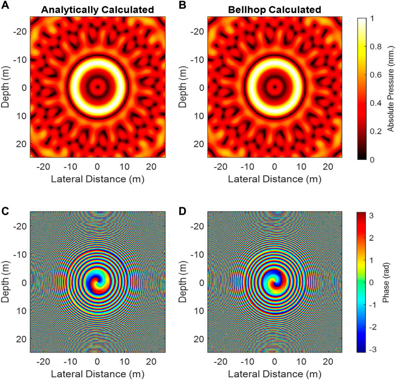
FIGURE 3. Absolute pressure and phase relationships for the same array calculated analytically (A,C) and using BELLHOP (B,D) for the same array at a range of 100 m.

5 Applications and examples

A brief discussion of the comparative computational advantage when compared to finite element methods does well to point out the value of these methods and the extent of their applications. Finite element methods fundamentally require numerical evaluations at each point in a densely populated mesh (each case is unique, however the mesh size is always fractions of a wavelength). Figures 1, 3 were calculated over a range of 1,000 wavelengths for a depth axis of 500 wavelengths and an out of plane distance of 500 wavelengths. To compute these two figures using finite elements (assuming a mesh size of six samples per wavelength), 54 billion point-wise evaluations would be required. These ray tracing methods require the pressure calculation at the number of field points required for the plot being produced. Figure 3 had a dimensionality of 1,500 × 1,500 points. Ignoring symmetry (which can be exploited to drive the number of points down by as much as half for some of the transducers in the array), calculating these field points for 48 transducers results in 108 million point-wise computations plus the relatively simple calculation of ray trajectories. Not only are fewer evaluation points required for the ray trace, but their values are far simpler to produce. When the effects of increasing range and frequency are considered, finite element methods quickly become untenable, while the ray tracing methods remain relatively simple by comparison.

5.1 Inhomogeneous and multipath environments

To this point, the examples presented have been limited to relatively simple environments to illustrate the methods and show their efficacy. As presented in (Fan et al., 2019; Kelly and Shi, 2023), these methods may also be applied effectively to more realistic environments. Here an even more complex environment is presented to illustrate the robustness of these methods. We explore the performance of an array in a 500 m deep ocean environment in the presence of a strong acoustic duct over various ranges and for two array depths. Figure 5 shows the results of the array transmitting l = +2 at ranges of 500m and 1000 m for an array centered on the duct. To illustrate the effects of refraction, the vortex is depicted at a range of 500 m for an array offset by 50 m from the duct center. Based on the results of Kelly and Shi (Kelly and Shi, 2023), we also maintain the rings of the array in phase with the innermost ring for the improved performance. Eq. 3 shows the phase relationship for transducers in a given ring.

${\theta }_n=\frac{2\pi ln}{N}(3)$

Previous published examples have focused on vortex beams centered in an acoustic duct. This is a logical starting point because acoustic ducts are inherently supportive of long-range propagation, and the fragile phase relationships which are required of a propagating vortex will be largely maintained. Environmental conditions may be such that in situ awareness of the true center of the duct will be difficult, and many platforms are not designed to operate at depths consistent with a deep sound channel axis (or SOFAR channel). These methods suggest that the vortex can be tracked and appropriately reconstructed even in cases where the medium is generally refractive. Interestingly, in the off-axis case (Figure 4 g & h), the phase pattern shifts from the standard bladed appearance to the forked interference pattern. This pattern is oft reported in the optics community as the result of the interaction between a vortex wave and a plane wave, the results of which are well described in (Lv et al., 2018). This pattern has been observed in the acoustics community in (Zou et al., 2020b) where the imaging plane of a vortex is not perpendicular to the propagation direction. In (Zou et al., 2020b) the authors measured an acoustic vortex which was reflected off the air-water interface and imaged the field such that the vortex passed through the imaging plane at an angle. This work also presented methods for projecting the forked interference pattern back onto the propagating plane for proper evaluation. Here the imaging plane is perpendicular to the range axis, so as the vortex beam refracts downward away from the positive gradient in sound speed profile, the orientation of the vortex is no longer perfectly aligned with the imaging plane. In either case, the topological charge can be resolved from the phase pattern.

FIGURE 4

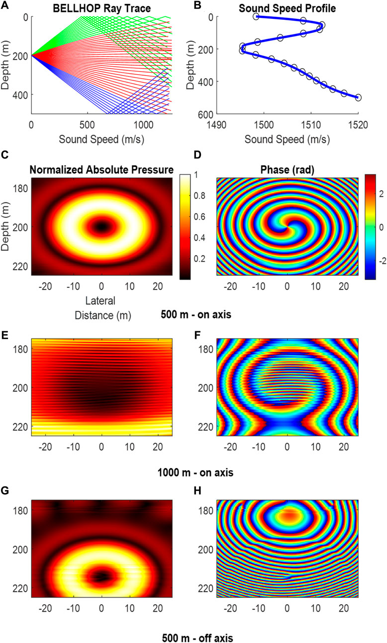
FIGURE 4. Amplitude and phase relationships for 15 kHz vortex wave emitted along the central axis (200 m in depth) of an acoustic duct at a range of 500 m (C–D) 1000 m (E–F). Additionally, the effects of a refracting vortex are depicted for an array centered at 150 m in depth and a range of 500 m (G–H). A ray trace (A) along with the environment sound speed profile (B) indicate the interference at 1000 m is being caused by the surface reflected propagation path. Phase relationships established in Kelly and Shi were used for these plots.

These methods also allow for a more in-depth analysis of the pressure fields including signal processing applications. To demonstrate this, simple k-space filtering techniques are applied to a propagating vortex in a multi-path environment. A unit-step mask (marked by the intersection of the red dashed lines in Figure 5C) is applied to the k-space for the vortex in order to isolate the direct path. Figure 5 shows the results of this analysis.

FIGURE 5

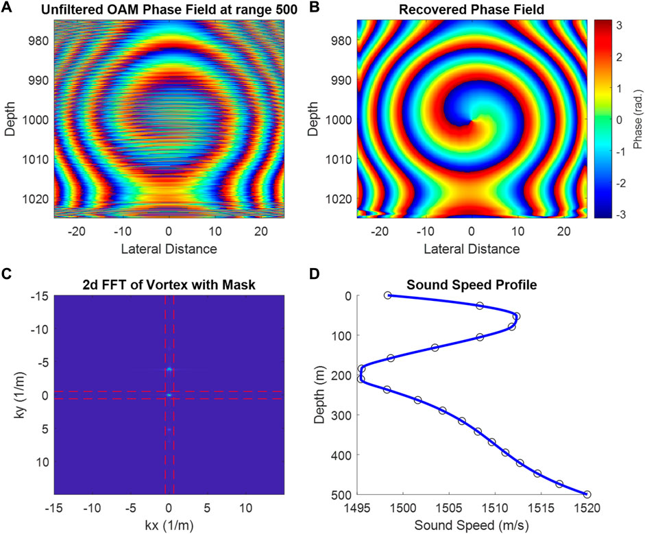
FIGURE 5. The effects of k-space filtering a propagating vortex with a distorted phase field caused by multipath propagation. The distorted phase field (A) is filtered using a unit-step mask (C) in order to recover the phase field (B). The sound speed profile for the environment is depicted in (D). Phase relationships established in Kelly and Shi were used for these plots.

Despite significant distortion caused by the multi-path propagation environment, the vortex is faithfully recovered using the mask to isolate the direct path signal. This demonstrates the ability to use these simulation methods as a tool to explore the signal processing challenges that are inherent with long-range vortex propagation.

6 Conclusion

We present methods that compute acoustic vortex beams over long-range propagation efficiently. By employing BELLHOP’s ray tracing algorithms, both range vs. depth and wavefront propagating plots of propagating acoustic vortices can be resolved in environments of varying complexity. Example cases considering multipath and refractive environments are also presented. The example cases provide evidence to these methods as a robust and reliable tool for simulating the long-range propagation of acoustic vortex beams in complex environments.

Data availability statement

The original contributions presented in the study are included in the article/Supplementary Material, further inquiries can be directed to the corresponding author.

Author contributions

MK: Conceptualization, Data curation, Formal Analysis, Investigation, Methodology, Validation, Visualization, Writing–original draft. ZZ: Conceptualization, Methodology, Writing–review and editing. LZ: Conceptualization, Methodology, Writing–review and editing. CS: Conceptualization, Funding acquisition, Investigation, Methodology, Project administration, Resources, Supervision, Writing–review and editing.

Funding

The author(s) declare financial support was received for the research, authorship, and/or publication of this article. MK and CS are supported by the Office of Naval Research under grant number N00014-22-1-2551.

Conflict of interest

The authors declare that the research was conducted in the absence of any commercial or financial relationships that could be construed as a potential conflict of interest.

Publisher’s note

All claims expressed in this article are solely those of the authors and do not necessarily represent those of their affiliated organizations, or those of the publisher, the editors and the reviewers. Any product that may be evaluated in this article, or claim that may be made by its manufacturer, is not guaranteed or endorsed by the publisher.

Supplementary material

The Supplementary Material for this article can be found online at: https://www.frontiersin.org/articles/10.3389/facou.2023.1292050/full#supplementary-material

References

Cain, C. A., and Umemura, S. (1986). Concentric-ring and sector-vortex phased-array applicators for Ultrasound hyperthermia. IEEE Trans. Microw. Theory Tech. 34 (5), 542–551. doi:10.1109/TMTT.1986.1133390

CrossRef Full Text | Google Scholar

Durnin, J., Miceli, J., and Eberly, J. (1987) Diffraction-free beams. Phys. Rev. Lett. 58, 1499–1501. doi:10.1103/PhysRevLett.58.1499

PubMed Abstract | CrossRef Full Text | Google Scholar

Fan, X., Zou, Z., and Zhang, L. (2019). Acoustic vortices in inhomogeneous media. Phys. Rev. Res. 1, 032014. doi:10.1103/PhysRevResearch.1.032014

CrossRef Full Text | Google Scholar

Fan, X. D., and Zhang, L. (2019). Trapping force of acoustical Bessel beams on a sphere and stable tractor beams. Phys. Rev. Appl. 11, 014055. doi:10.1103/physrevapplied.11.014055

CrossRef Full Text | Google Scholar

Guo, S., Ya, Z., Wu, P., and Wan, M. (2022b). A review on acoustic vortices: generation, characterization, applications and perspectives. J. Appl. Phys. 132 (21), 210701. doi:10.1063/5.0107785

CrossRef Full Text | Google Scholar

Guo, S., Ya, Z., Wu, P., Zhang, L., and Wan, M. (2022). Enhanced sonothrombolysis induced by high-intensity focused acoustic vortex. Ultrasound Med. Biol. Sep. 48 (9), 1907–1917. doi:10.1016/j.ultrasmedbio.2022.05.021

CrossRef Full Text | Google Scholar

Hefner, B. T., and Marston, P. L. (1999). An acoustical helicoidal wave transducer with applications for the alignment of ultrasonic and underwater systems. J. Acoust. Soc. Am. 106, 3313–3316. doi:10.1121/1.428184

CrossRef Full Text | Google Scholar

Jensen, F. B., Kuperman, W. A., Porter, M. B., Schmidt, H., and Bartram, J. F. (1995). Computational Ocean acoustics. J. Acoust. Soc. Am. 97, 3213–3215. doi:10.1121/1.411832

CrossRef Full Text | Google Scholar

Kelly, M. E., and Shi, C. (2023). Design and simulation of acoustic vortex wave arrays for long-range underwater communication. JASA Express Lett. 3 (7), 076001. doi:10.1121/10.0019884

PubMed Abstract | CrossRef Full Text | Google Scholar

Lo, W. C., Fan, C. H., Ho, Y. J., Lin, C. W., and Yeh, C. K. (2021). Tornado-inspired acoustic vortex tweezer for trapping and manipulating microbubbles. Proc. Natl. Acad. Sci. U.S.A. 118, e2023188118. doi:10.1073/pnas.2023188118

PubMed Abstract | CrossRef Full Text | Google Scholar

Lv, R., Qiu, L., Hu, H., Meng, L., and Zhang, Y. (2018). The phase interrogation method for optical fiber sensor by analyzing the fork interference pattern. Appl. Phys. B 124, 32. doi:10.1007/s00340-018-6901-5

CrossRef Full Text | Google Scholar

Shi, C., Dubois, M., Wang, Y., and Zhang, X. (2017). High-speed acoustic communication by multiplexing orbital angular momentum. Proc. Natl. Acad. Sci. 114, 7250–7253. doi:10.1073/pnas.1704450114

PubMed Abstract | CrossRef Full Text | Google Scholar

Umemura, S., and Cain, C. A. (1989). The sector-vortex phased array: acoustic field synthesis for hyperthermia. IEEE Trans. Ultrason. Ferroelectr. Freq. Control 36 (2), 249–257. doi:10.1109/58.19158

PubMed Abstract | CrossRef Full Text | Google Scholar

Zhang, B., Hong, Z., and Drinkwater, B. (2022). Transfer of orbital angular momentum to freely levitated high-density objects in airborne acoustic vortices. Phys. Rev. Appl. 18, 024029. doi:10.1103/physrevapplied.18.024029

CrossRef Full Text | Google Scholar

Zhang, B., Wu, H., Kim, H., Welch, P. J., Cornett, A., Stocker, G., et al. (2023). A model of high-speed endovascular sonothrombolysis with vortex ultrasound-induced shear stress to treat cerebral venous sinus thrombosis. Research 6, 0048. doi:10.34133/research.0048

PubMed Abstract | CrossRef Full Text | Google Scholar

Zhang, L., and Marston, P. L. (2011). Angular momentum flux of nonparaxial acoustic vortex beams and torques on axisymmetric objects. Phys. Rev. E 84 (6), 065601. doi:10.1103/physreve.84.065601

PubMed Abstract | CrossRef Full Text | Google Scholar

Zou, Z., Fan, X., and Zhang, L. (2020a). Modeling underwater propagation of acoustic vortex beams by ray methods. J. Acoust. Soc. Am. 148, 2563. doi:10.1121/1.5147112

CrossRef Full Text | Google Scholar

Zou, Z., Lirette, R., and Zhang, L. (2020b). Orbital angular momentum reversal and asymmetry in acoustic vortex beam reflection. Phys. Rev. Lett. 125, 074301. doi:10.1103/physrevlett.125.074301

PubMed Abstract | CrossRef Full Text | Google Scholar