Sequential Imputation of Missing Spatio-Temporal Precipitation Data Using Random Forests

Meteorological records, including precipitation, commonly have missing values. Accurate imputation of missing precipitation values is challenging, however, because precipitation exhibits a high degree of spatial and temporal variability. Data-driven spatial interpolation of meteorological records is an increasingly popular approach in which missing values at a target station are imputed using synchronous data from reference stations. The success of spatial interpolation depends on whether precipitation records at the target station are strongly correlated with precipitation records at reference stations. However, the need for reference stations to have complete datasets implies that stations with incomplete records, even though strongly correlated with the target station, are excluded. To address this limitation, we develop a new sequential imputation algorithm for imputing missing values in spatio-temporal daily precipitation records. We demonstrate the benefits of sequential imputation by incorporating it within a spatial interpolation based on a Random Forest technique. Results show that for reliable imputation, having a few strongly correlated references is more effective than having a larger number of weakly correlated references. Further, we observe that sequential imputation becomes more beneficial as the number of stations with incomplete records increases. Overall, we present a new approach for imputing missing precipitation data which may also apply to other meteorological variables.

Introduction

Precipitation is an important component of the ecohydrological cycle and plays a crucial role in driving the Earth's climate. It serves as an input for various ecohydrological models to determine snowpack, infiltration, surface-water flow, groundwater recharge, and transport of chemicals, sediments, nutrients, and pesticides (Devi et al., 2015). Numerical modeling of surface flow typically requires a complete time series of precipitation along with other meteorological records (e.g., temperature, relative humidity, solar radiation) as inputs for simulations (Dwivedi et al., 2017, 2018; Hubbard et al., 2018, 2020; Zachara et al., 2020). However, meteorological records often have missing values for various reasons, such as due to malfunctioning of equipment, network interruptions, and natural hazards (Varadharajan et al., 2019). Missing values need to be reconstructed or imputed accurately to ensure that estimates of statistical properties, such as mean and co-variance, are consistent and unbiased (Schneider, 2001) because inaccurate estimates can hurt the accuracy of ecohydrological models. Reconstructing an incomplete daily precipitation time series is especially difficult since it exhibits a high degree of spatial and temporal variability (Simolo et al., 2010).

Past efforts for imputing missing values of a precipitation time series fall under two broad categories: autoregression of univariate time series and spatial interpolation of precipitation records. Autoregressive methods are self-contained and impute missing values by using data from the same time series that is being filled. Simple applications could involve using a mean value of the time series, or using data from 1 or several days before and after the date of missing data (Acock and Pachepsky, 2000). More sophisticated versions of autoregressive approaches implement stochastic methods and machine learning (Box and Jenkins, 1976; Adhikari and Agrawal, 2013). To illustrate some recent studies, Gao et al. (2018) highlighted methods to explicitly model the autocorrelation and heteroscedasticity (or changing variance over time) of hydrological time series (such as precipitation, discharge, and groundwater levels). They proposed the use of autoregressive moving average models and autoregressive conditional heteroscedasticity models. Chuan et al. (2019) combined a probabilistic principal component analysis model and an expectation-maximization algorithm, which enabled them to obtain probabilistic estimates of missing precipitation values. Gorshenin et al. (2019) used a pattern-based methodology to classify dry and wet days, then filled in precipitation for wet days using machine learning approaches (such as k-nearest neighbors, expectation-maximization, support vector machines, and random forests). However, an overarching limitation of autoregressive methods is the need for the imputed variable to show a high temporal autocorrelation, which is not necessarily valid for precipitation (Simolo et al., 2010). Therefore, such methods have limited applicability when it comes to reconstructing a precipitation time series.

Spatial interpolation methods, on the other hand, impute missing values at the target station by taking weighted averages of synchronous data, i.e., data at the same time, from reference stations (typically neighboring stations). The success of these methods relies on the existence of strong correlations among precipitation patterns between the target and reference stations. The two most prominent approaches are inverse-distance weighting (Shepard, 1968) and normal-ratio methods (Paulhus and Kohler, 1952). The inverse-distance weighting assumes the weights to be proportional to the distance from the target, while the normal-ratio method assumes the weights to be proportional to the ratio of average annual precipitation at the target and reference stations. Another prominent interpolation approach is based on kriging or gaussian processes, which assigns weights by accounting for spatial correlations within data (Oliver and Webster, 2015). Teegavarapu and Chandramouli (2005) proposed several improvements to weighting methods and also introduced the coefficient of correlation weighting method—here the weights are proportional to the coefficient of correlation with the target. Recent studies have proposed new weighting schemes using more sophisticated frameworks (e.g., Morales Martínez et al., 2019; Teegavarapu, 2020). In parallel, studies have also been conducted to account for various uncertainties in imputation. For example, Ramos-Calzado et al. (2008) proposed a weighting method to account for measurement uncertainties in a precipitation time series. Lo Presti et al. (2010) proposed a methodology to approximate each missing value by a distribution of values where each value in the distribution is obtained via a univariate regression with each of the reference stations. Simolo et al. (2010) pointed out that weighting approaches have a tendency to overestimate the number of rainy days and to underestimate heavy precipitation events. They addressed this issue by proposing a spatial interpolation procedure that systematically preserved the probability distribution, long-term statistics, and timing of precipitation events.

A critical review of the literature shows that, in general, spatial interpolation techniques have two fundamental shortcomings: (i) how to optimally select neighbors, i.e., reference stations, and (ii) how to assign weights to selected stations. While selecting reference stations is typically done using statistical correlation measures, assigning weights to selected stations is currently an ongoing area of research. The methods reviewed so far are based on the idea of specifying a functional form of the weighting relationships. The appropriate functional form may vary from one region to another depending on the prevalent patterns of precipitation as influenced by local topographic and convective effects. Using a functional form that is either inappropriate or too simple could distort the statistical properties of the datasets (such as mean and covariance). Some researchers have proposed to address these shortcomings by using Bayesian approaches (e.g., Yozgatligil et al., 2013; Chen et al., 2019; Jahan et al., 2019). These fall under the broad category of expectation-maximization and data augmentation algorithms, thus yielding a probability distribution for each missing value.

An alternative approach for imputing missing data is the application of data-driven or machine learning (ML) methods which are becoming increasingly prominent for imputing using spatial interpolation. These methods do not need a functional form to be specified a priori and can learn a multi-variate relationship between the target station and reference stations using available datasets. Studies have found that the performance of ML methods tends to be superior to that of traditional weighting methods (e.g., Teegavarapu and Chandramouli, 2005; Hasanpour Kashani and Dinpashoh, 2012; Londhe et al., 2015). In addition, studies have been conducted to identify an optimal architecture for ML-based methods (Coulibaly and Evora, 2007; Kim and Pachepsky, 2010). In this work, we use a Random Forests (RF) method. The RF is an ensemble learning method which reduces associated bias and variance, making predictions less prone to overfitting. In addition, a recent study showed that RF-based imputation is generally robust, and performance improves with increasing correlation between the target and references (Tang and Ishwaran, 2017).

Regardless of the imputation technique, an inherent limitation of spatial interpolation algorithms is the need for reference stations to have complete records during the time-period of interest. This limitation is critical for ML algorithms where incomplete records preclude data-driven learning of multi-variate relationships. The success of spatial interpolation, therefore, depends on whether precipitation at the target station is highly correlated with precipitation at stations with complete records. A station with an incomplete record is typically excluded from the analysis even though that station may have a high correlation with the target station. In this work, we hypothesize that stations with incomplete records contain information that can improve spatial interpolation if they are included in the analysis. We propose a new algorithm, namely sequential imputation, that leverages incomplete records to impute missing values. In this approach, stations that are imputed first are also included as reference stations for imputing subsequent stations. We implement this algorithm in the context of imputing missing daily values of precipitation and demonstrate its benefits by incorporating it in an RF-based spatial interpolation.

In what follows, we start by describing our study area and data sources and follow this with a brief introduction to the Random Forests (RF) method. We then describe all our numerical experiments, starting with a baseline imputation that helps evaluate the performance of sequential imputation. This is followed by a description of the sequential imputation algorithm, along with an outline of different scenarios to evaluate sequential imputation. We compare the results of sequential imputation with a non-sequential imputation in which incomplete records are not leveraged for subsequent imputations. Finally, we discuss the implications of our results and provide some concluding thoughts.

Methodology

Study Area and Data Sources

We conducted this study using data from the Upper Colorado Water Resource Region (UCWRR), which is one of 21 major water resource regions classified by the United States Geological Survey to divide and sub-divide the United States into successively smaller catchment areas. The UCWRR is the principal source of water in the southwestern United States and includes eight subregions, 60 sub-basins, 523 watersheds, and 3,179 sub-watersheds. Several agencies have active weather monitoring stations in UCWRR. For our study, we considered the weather stations maintained by the Natural Resources Conservation Service (NRCS). Table 1 summarizes the various networks that comprise the NRCS database.

TABLE 1

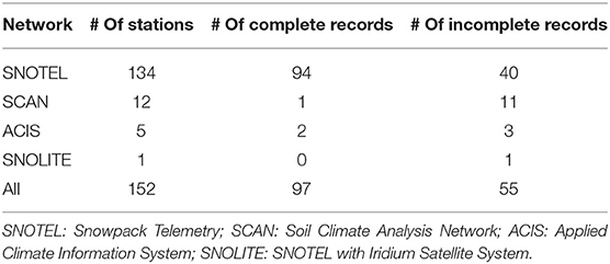
Table 1. Summary of NRCS stations in UCWRR.

Figure 1 shows the spatial distribution of NRCS stations in UCWRR. Ninety-seven stations have complete records which primarily belong to the Snowpack Telemetry (SNOTEL) network. We considered data spanning the 10-year window from 2008 to 2017. Over this period, NRCS had 152 active stations in UCWRR which report daily precipitation data. For this study, our dataset is restricted to the 97 stations with complete records. We downloaded the data through the NRCS Interactive Map and Report Generator¹ (accessed Jan 16, 2020).

FIGURE 1

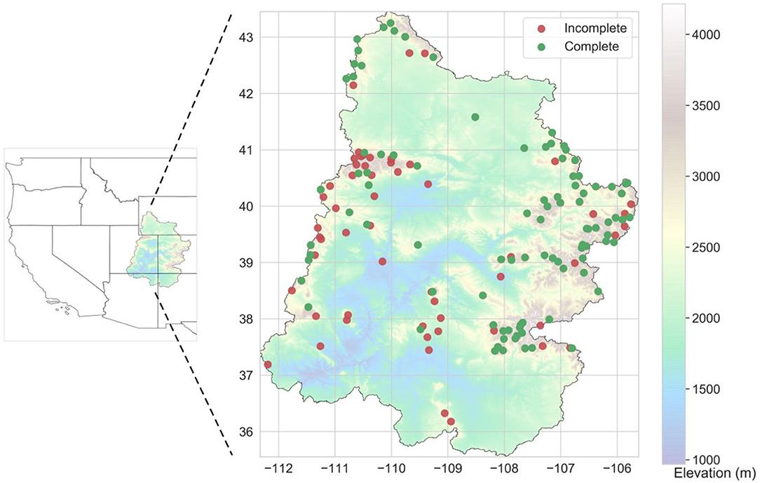
Figure 1. Spatial extent of UCWRR, along with the layout of stations in the NRCS database (comprising of 97 complete and 55 incomplete records).

Spatial Interpolation Method: Random Forests (RF)

RF is an ML-method based on an ensemble or aggregation of decision-trees (Breiman, 2001). A decision-tree is a flowchart-like structure that recursively partitions the input feature space into smaller subspaces (Figure 2). Recursion is carried out till the subspaces are small enough to fit simple linear models on them In regression problems, the decision rules for partitioning are determined such that the mean-squared error between the tree output and the observed output is minimized. The RF model trains each decision-tree on a different set of data points obtained by sampling the training data with replacement (or bootstrapping). Furthermore, each tree may also consider a different subset of input features selected randomly. The final output of the random forest is obtained by aggregating (or ensembling) the results of all decision trees. For regression problems, aggregation is done by taking the mean. Figure 2 shows a schematic of an RF regressor.

FIGURE 2

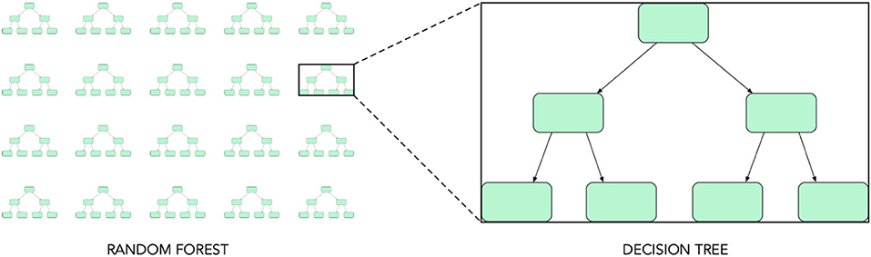
Figure 2. Schematic of a Random Forest regressor, adapted from Stockman et al. (2019).

The ensemble nature of RF leads to several benefits (Breiman, 2001; Louppe, 2015). First, it makes RF less prone to overfitting, despite the susceptibility of individual trees to overfitting (Segal, 2004). For regression problems, overfitting refers to low values of mean-squared error on training data, and high values of mean-squared error on test data. Second, it enables an evaluation of the relative importance of a variable (which, in this work, refers to a reference station) for predicting the output. This is typically done by determining how often a variable is used for partitioning the input feature space, across all trees. Third, the ensemble nature of RF makes it possible to not set aside a test set. Since the input for each decision tree is obtained by bootstrapping, the unsampled data can be used to estimate the generalization error. In addition, RF does not require extensive hyperparameter tuning compared to other ML approaches (Ahmad et al., 2017).

In this study, we implement RF using Python's scikit-learn module (Pedregosa et al., 2011). Precipitation data from reference stations acts as input, and precipitation data at the target station is specified as the output. Unlike typical spatial interpolation approaches, we do not specify distances between the reference and target stations. Distances are static variables and their influence on dynamic precipitation relationships gets learnt as a constant bias, regardless of whether they are explicitly specified or not.

Overview of Numerical Experiments

To investigate if stations with incomplete records contain information that can improve spatial interpolation, we designed three sets of numerical experiments: baseline, sequential, and non-sequential imputation. In baseline imputation, each station in our dataset is modeled using the remaining stations as reference stations. This represents an upper bound on the performance of sequential imputation when we have multiple stations with incomplete records. The baseline imputation provides statistics to help evaluate the performance of sequential imputation. In sequential imputation, a subset of stations in our dataset is marked as artificially incomplete. For each station in the artificially incomplete subset, 20% of the values are randomly marked as “missing.” The missing values are imputed by leveraging other artificially incomplete stations in the subset, in addition to using stations outside the subset. Finally, in non-sequential imputation, the same artificially incomplete subset as sequential imputation is considered, and missing values are imputed using just the stations that are outside the subset. We describe the three sets of numerical experiments in detail in sections Numerical Experiments: Baseline Imputation and Numerical Experiments: Sequential and Non-sequential Imputation. Before describing each of these experiments, it would be instructive to discuss our performance criterion for evaluating imputation.

Evaluating Imputation: Nash-Sutcliffe Efficiency (NSE)

We evaluated the overall performance of imputation by computing the Nash-Sutcliffe Efficiency (NSE) on test data given by

$\begin{array}{ll}NSE=1-\frac{{\displaystyle {\sum }_{i=1}^N}{\left(y_i^o-y_i^m\right)}^2}{{\displaystyle {\sum }_{i=1}^N}{\left(y_i^o-\overline{y^o}\right)}^2}& (1)\end{array}$

where N is the size of the test set, $y_i^o$ is i-th observed value, $y_i^m$ is the corresponding modeled value, and $\overline{y^o}$ is the mean of all observed values in the test set.

The NSE is a normalized statistical measure that determines the relative magnitude of the residual variance (or noise) of a model when compared to the measured data variance. It is dimensionless and ranges from −∞ to 1. An NSE value equal to 1 implies that the modeled (in our case, imputed) values perfectly match the observations; an NSE value equal to 0 implies that the modeled values are only as good as the mean of observations; and a negative NSE value implies that the mean of observations is a better predictor than modeled values. Positive NSE values are desirable, and higher values imply greater accuracy of the (imputation) model.

Two other common statistical measures for evaluating the overall accuracy of prediction are Pearson's product-moment correlation coefficient R, and the Kolmogorov-Smirnov statistic. While the former evaluates the timing and shape of the modeled time series, the latter evaluates its cumulative distribution. Gupta et al. (2009) decomposed the NSE into three distinctive components representing the correlation, bias, and a measure of relative variability in the modeled and observed values. They showed that NSE relates to the ability of a model to reproduce the mean and variance of the hydrological observations, as well as the timing and shape of the time series. For these reasons, the use of NSE was preferred over other statistical measures to evaluate the accuracy of imputation.

We also evaluated the performance of sequential imputation for predicting dry events and extreme wet events. This is because spatial interpolation approaches tend to overpredict the number of dry events and underestimate the intensity of extreme wet events (Simolo et al., 2010; Teegavarapu, 2020). A common practice is to consider a day as a dry event if the daily precipitation does not exceed a threshold of 1 mm (Hertig et al., 2019). We considered a threshold of 2.54 mm since that is the resolution of our dataset. We considered a day as an extreme wet event if the daily precipitation exceeded the 95th percentile of the entire precipitation record for a given station (Zhai et al., 2005; Hertig et al., 2019). To evaluate prediction accuracy for dry events, we computed the percentage error, or the percentage of days that were correctly modeled as dry days. To evaluate prediction accuracy for extreme wet events, we computed NSE values exclusively for days that exceeded the 95th percentile of daily precipitation values; this enabled us to evaluate the predicted magnitude. In what follows, we use the acronym NSEE to denote NSE for extreme events.

Numerical Experiments: Baseline Imputation

For our first set of numerical experiments, we conducted baseline imputations where each station in our dataset is modeled using the remaining stations as reference stations. Our dataset consists of 97 stations with complete records (as outlined in Figure 1 and Table 1). This set of numerical experiments is a test of the RF-based imputation method and provides an upper bound on the performance of the sequential imputation algorithm discussed in the section Sequential Imputation Algorithm. More importantly, it provides estimates of the variance for modeling each station, which will be used to evaluate the performance of the sequential imputation algorithm. Specifically, each station in our dataset was considered, in turn, to be a target station (or model output), with the rest of the stations acting as references (or input features). For each target station, 80% of the data were randomly selected for training, and the remaining 20% were used for testing. The test set effectively acted as missing data to be imputed. We conducted this exercise 15 times for each station. Prior to these runs, we also conducted an independent set of baseline runs to tune the hyperparameters of RF.

Sequential Imputation Algorithm

ML-based spatial interpolation learns multi-variate relationships between the reference stations and the target station. Studies have noted that for imputation results to be reliable, data at reference stations should be strongly correlated to data at the target station (e.g., Teegavarapu and Chandramouli, 2005; Yozgatligil et al., 2013). However, ML-based spatial interpolation excludes stations that have incomplete records, even though they may be strongly correlated with the target station. Here, we develop a technique (i.e., sequential imputation) where stations that are imputed first are used as reference stations for imputing subsequent stations. In what follows, we refer to a station with a complete record as a “complete station,” and a station with an incomplete record as an “incomplete station.” The sequential imputation algorithm involves the following steps:

1. Add all complete stations to the list of reference stations.

2. Calculate correlations between incomplete stations and reference stations.

3. Pick the incomplete station having the highest aggregate correlation with reference stations.

4. Impute missing values for the station picked in Step 3, using all the reference stations.

5. Add the imputed station to the list of reference stations.

6. Repeat steps 2–4 till missing values of all the stations are imputed.

In this study, correlation refers to Pearson's product-moment correlation coefficient, hereafter denoted by R. We chose this measure for its simplicity. Step 3 requires calculating an aggregate correlation of each incomplete station with the reference stations. This step assumes that the incomplete station having the highest aggregate correlation with reference stations will have the most accurate imputation. We will verify this assumption in the Results section. To determine an appropriate aggregate correlation measure for Step 3, we implemented the following procedure:

i. Compute correlations of a target station with each of the reference stations.

ii. Sort the correlation values in descending order (highest to lowest).

iii. Calculate the cumulative sum of the sorted correlations. Denote each partial sum as S_i, where subscript i refers to the first i sorted correlations.

i varies from 1 to N, and N is the number of reference stations in the dataset. Each S_i is an aggregate measure of correlation between a target station and the reference stations. For instance, S₂ refers to the sum of first two sorted correlations, S₃ refers to the sum of first three sorted correlations, and so on. We computed values of S_i for all the 97 stations in our dataset and compared their values with NSE determined from baseline imputations. The S_i having the highest correlation with NSE was picked to quantify aggregate correlation (for Step 3 of sequential imputation). For practical applications, the above procedure to determine an appropriate aggregate correlation may be implemented using non-sequential imputations. Note that other aggregate measures may be envisioned (e.g., mutual information, spearman's correlation), but we sought to pick one that is relatively simple to keep our focus on the sequential imputation approach.

Numerical Experiments: Sequential and Non-sequential Imputation

To investigate the benefits of sequential imputation, we divided our dataset of 97 complete stations into five (almost) evenly sized subsets and labeled them 1 through 5, as shown in Figure 3. The division into subsets was random. We then considered four different scenarios, each of which marked certain subsets as artificially incomplete. These are shown in Table 2.

FIGURE 3

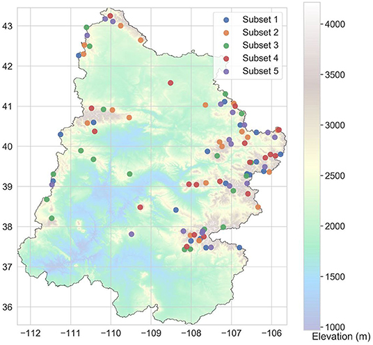
Figure 3. Division of complete stations (see Figure 1) into five subsets.

TABLE 2

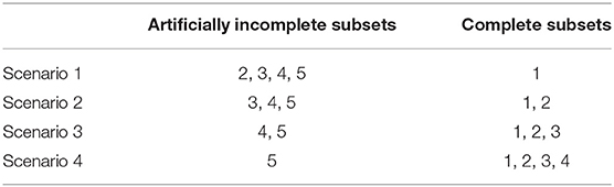
Table 2. Scenarios for sequential and non-sequential imputation.

Precipitation records typically have missing values resulting from random mechanisms such as malfunctioning of equipment, network interruptions, and natural hazards. In other words, the probability that a precipitation value is missing does not depend on the value of precipitation itself. These random mechanisms also assume that the location or physiography of a weather station has no bearing on whether its record is complete or incomplete. This missing at random mechanism (Schafer and Graham, 2002) is reflected in our decision to create subsets randomly, and enables us to evaluate the sequential imputation approach in a more generic setting.

Figures 4A–D shows the division of our dataset into complete and artificially incomplete subsets for each of the scenarios listed in Table 2. Scenario 1 had 77 out of 97 records marked as artificially incomplete. Each subsequent scenario had fewer records marked as artificially incomplete, culminating with Scenario 4 which had only 19 such records. These scenarios were designed to investigate how the proportion of incomplete records affects imputation. We expected sequential imputation to be more beneficial as the proportion of incomplete records increased in the dataset.

FIGURE 4

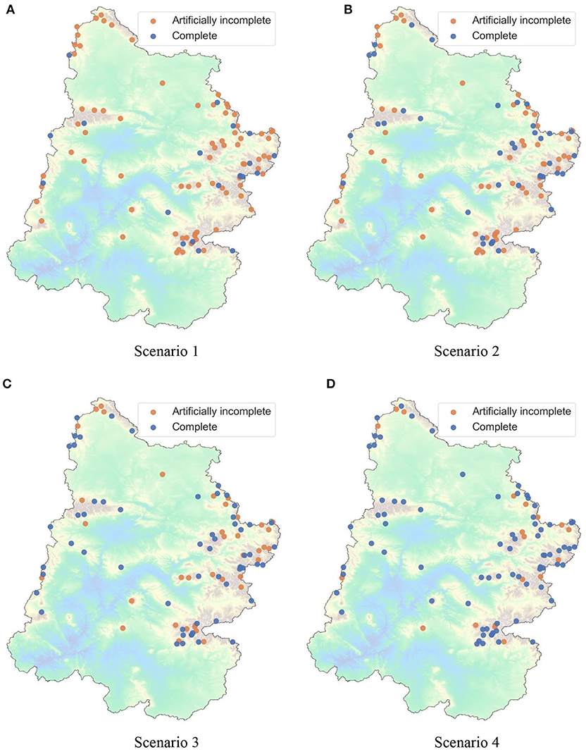
Figure 4. Artificially incomplete and complete datasets for different scenarios of sequential and non-sequential imputation. Note: Colormap for elevation is same as Figures 1, 3. (A) Scenario 1. (B) Scenario 2. (C) Scenario 3. (D) Scenario 4.

The stations belonging to the artificially incomplete subsets had 20% of their data marked as missing. Previous studies on imputation have considered two broad mechanisms for marking missing values. One approach involves marking missing values randomly (e.g., Teegavarapu and Chandramouli, 2005; Kim and Pachepsky, 2010), while the other approach assumes that missing values form continuous gaps in time (e.g., Simolo et al., 2010; Yozgatligil et al., 2013). Since spatial interpolation assumes no temporal autocorrelation and is agnostic to the timestamp of the data, the mechanism for marking missing values is not relevant. For simplicity, we assumed that values were missing completely at random. The missing values were imputed using sequential and non-sequential imputations; both these imputations were compared and enabled us to highlight the benefits of sequential imputation. Specifically, we calculated NSE corresponding to both sequential and non-sequential runs and computed the change (or increase) Δ in NSE for each station as follows:

$\begin{array}{ll}\Delta NSE=NS{E}_{\text{sequential}}-NS{E}_{\text{non-sequential}}& (2)\end{array}$

To evaluate improvement in prediction of extreme wet events, NSE in Equation 2 was replaced by NSEE. To evaluate improvement in prediction of dry days, we computed the percentage error (i.e., the percentage of days that were correctly modeled as dry days) corresponding to both sequential and non-sequential runs. We then computed the change (or decrease) Δ in percentage error (PE) as follows:

$\begin{array}{ll}\Delta PE=P{E}_{\text{non-sequential}}-P{E}_{\text{sequential}}& (3)\end{array}$

Results

Baseline Imputation

We performed baseline imputation to estimate statistics to evaluate the performance of the sequential imputation algorithm. Figures 5A–C show results of baseline imputations on missing data for all stations. Each station was modeled 15 times, with different splits of training and testing (missing) data, and the accuracy of each model for imputation was quantified by computing NSE on test data. This provided us with a distribution of NSE values (instead of just one value) for reconstructing each station, from which we estimated the mean μ and standard deviation σ of NSE for each station. For clarity, we denote the mean and standard deviation of a particular station s, by μ_s and σ_s, respectively. Figure 5A compiles the μ_s for all the stations and shows them as a histogram. Approximately 95% of the stations have a mean NSE >0.5, and approximately two-thirds of the stations have a mean NSE >0.65. Figure 5B compiles the μ_s and σ_s for all stations and shows them as a scatter plot. We see that for each station, the NSE values have a small standard deviation relative to their mean. Figure 5C shows the geospatial distribution of μ_s.

FIGURE 5

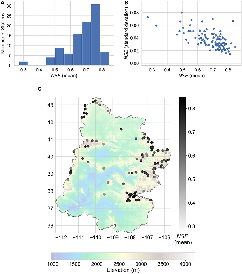
Figure 5. Results of baseline imputations on missing data. (A) Distribution of mean NSE (μ_s), (B) scatter of mean (μ_s), and standard deviation (σ_s) of NSE, (C) geospatial distribution of mean NSE (μ_s).

Figure 6 shows sample scatter plots of true and predicted precipitation on test data using baseline imputations. The dotted line shows the 45-degree line which corresponds to a perfect match (i.e., NSE = 1) between true and predicted values. Note that our dataset has a resolution of 0.1 inch or 2.54 mm, which results in visible jumps in the abscissa (or “true values”). Subfigure (a) corresponds to a relatively high value of NSE (~0.8), and subfigure (b) corresponds to a relatively low value of NSE (~0.5). We see from these plots that for a high value of NSE, the relative scatter is smaller and closer to the dotted line.

FIGURE 6

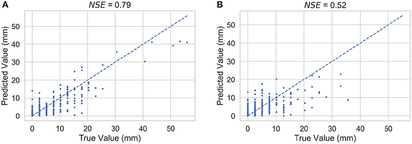
Figure 6. Sample scatter plots of true and predicted precipitation on test data using baseline imputations: (A) NSE = 0.79, (B) NSE = 0.52. Note that the jumps in true values are due to the coarse resolution (of 2.54 mm) of the dataset.

Aggregate Correlation Between Target Incomplete Stations and Reference Stations

To identify an appropriate aggregate correlation measure for sequential imputation, we analyzed results of baseline imputations. Specifically, we computed values of S_i for all the target stations (i.e., $S_i^s$) and compared their values with the corresponding μ_s. Since strong correlations with reference stations lead to more accurate imputation, we expect S_i to be positively correlated with μ, regardless of the value of i. As defined in the section Sequential Imputation Algorithm, S_i for a target station is the sum of first i sorted correlations with reference stations. For clarity, we denote $S_i^s$ to refer to S_i for a particular target station s. Figure 7A shows a scatter plot of $S_2^s$ and μ_s for all the stations in our dataset (as outlined in Figure 1 and Table 1). The correlation coefficient was 0.95. Similarly, we computed correlations between $S_i^s$ and μ_s for all values of i [denoted as $\text{Corr}({\mu }_s,S_i^s)]$, and plotted them in Figure 7B. These results show that the correlation between $S_i^s$ and μ_s is higher for lower values of i. On the basis of Figure 7, we used S₂ as the similarity measure for sequential imputation. For practical applications, an appropriate similarity measure may be determined by analyzing results of non-sequential imputations.

FIGURE 7

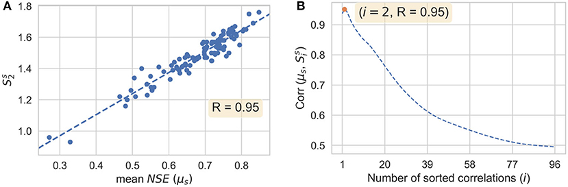
Figure 7. Quantifying similarity between target and reference stations: (A) scatter plot between $S_2^s$ and μ_s (mean value of NSE) with a linear fit, (B) correlations between μ_s and $S_i^s$ as a function of i (annotation: maximum value of the correlation).

Sequential Imputation

To implement the sequential imputation algorithm, the artificially incomplete subsets in each of the four scenarios were reconstructed using sequential and non-sequential imputation (see section Numerical Experiments: Sequential and Non-sequential Imputation). For a given station, sequential imputation was considered to have made a significant improvement if the corresponding Δ_sNSE (i.e., ΔNSE for station s computed using Equation 2) was greater than σ_s estimated from baseline runs. This was done to ensure that the change in NSE during sequential imputation may not be attributed to noise.

Figures 8A–11A show the results of sequential imputation for Scenarios 1–4, respectively, with values of NSE for each station corresponding to sequential imputation. The values are plotted in the order of sequential imputation and are superimposed over the baseline values of NSE. The baseline NSE curve is centered at its mean and the thickness represents its standard deviation (as shown in Figure 5B). The baseline curve provides an upper bound on the performance of the sequential imputation algorithm. Figures 8B–11B show change in NSE for each increment in sequence, when compared to a non-sequential imputation.

FIGURE 8

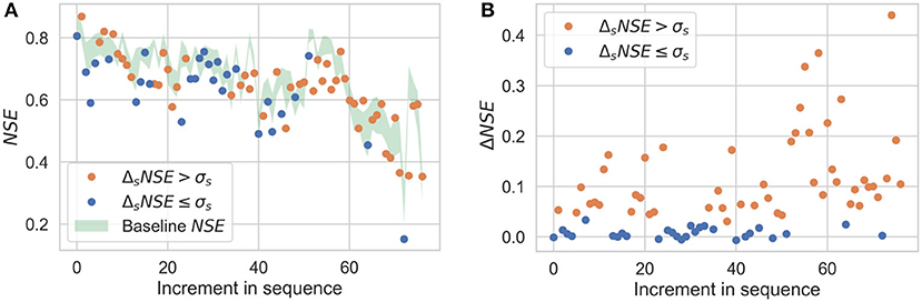
Figure 8. Sequential imputation results for Scenario 1. (A) NSE obtained during sequential imputation plotted as a function of increment in sequence and superimposed over baseline NSE values, (B) Change ΔNSE for each increment in sequence, when compared to a non-sequential imputation. Orange dots are considered significant improvements (i.e., Δ_sNSE > σ_s).

FIGURE 9

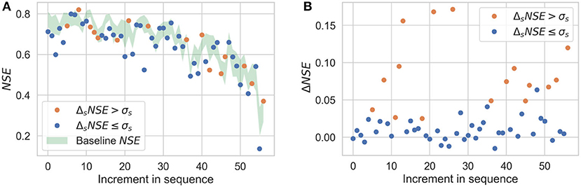
Figure 9. Sequential imputation results for Scenario 2; captions of (A,B) are same as in Figure 8.

FIGURE 10

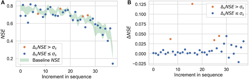
Figure 10. Sequential imputation results for Scenario 3; captions of (A,B) are same as in Figure 8.

FIGURE 11

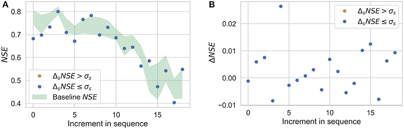
Figure 11. Sequential imputation results for Scenario 4; captions of (A,B) are same as in Figure 8.

Results for the scenarios are summarized in Table 3.

TABLE 3

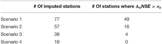
Table 3. Summary of results for Scenarios 1–4 for sequential and non-sequential imputation.

Figure 12 shows scatter plots of true and predicted precipitation on test data for a station that showed significant improvement during sequential imputation in Scenario 1. Subfigure (a) shows the scatter for non-sequential imputation, and subfigure (b) shows the scatter for sequential imputation. The dotted line shows the 45-degree line which corresponds to a perfect match (i.e., NSE = 1) between true and predicted values. Recall that our dataset has a resolution of 0.1 inch or 2.54 mm, which results in visible jumps in the abscissa (or “true values”).

FIGURE 12

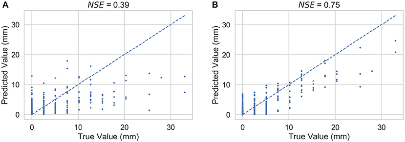
Figure 12. Scatter plots of true and predicted precipitation on test data for a station that showed significant improvement during sequential imputation in Scenario 1: (A) non-sequential imputation, (B) sequential imputation. Jumps in true values are due to the coarse resolution (of 2.54 mm) of the dataset.

Figures 13, 14 show the results of sequential imputation for predicting dry [subfigures (a)] and extreme wet [subfigures (b)] events for Scenarios 1, 2. The values are plotted in the order of sequential imputation and denote the change in PE or NSEE during sequential imputation when compared to a non-sequential imputation. The Δ values are color-coded according to results of Figures 8–11. The results for Scenarios 3, 4 are not shown for the sake of brevity.

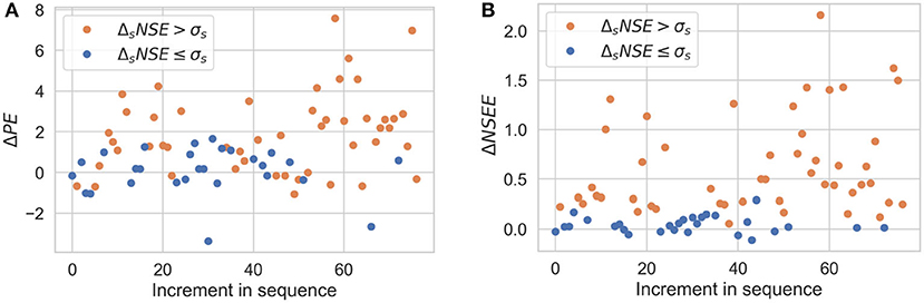
Figure 13. Sequential imputation results for predicting dry (A) and extreme wet (B) events for Scenario 1. Orange dots correspond to significant improvements in overall predictions as shown in Figure 8.

FIGURE 14

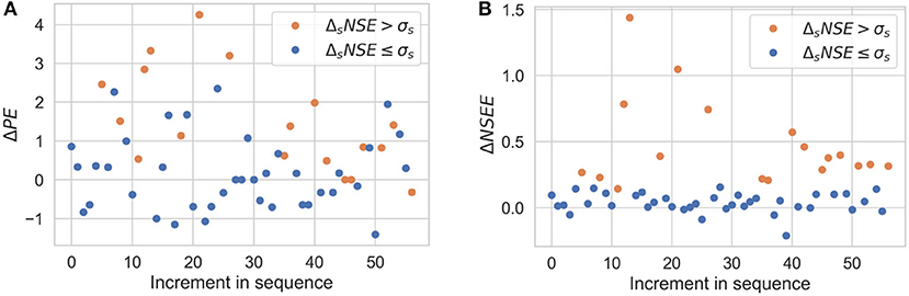
Figure 14. Sequential imputation results for predicting dry (A) and extreme wet (B) events for Scenario 2. Orange dots correspond to significant improvements in overall predictions as shown in Figure 9.

Discussion

Figure 5A shows the mean NSE (μ_s) for all the stations as a histogram. As noted earlier, approximately 95% of the stations have μ_s >0.5, and approximately two-thirds of the stations have a μ_s >0.65. Moriasi et al. (2007) reviewed over twenty studies related to watershed modeling and recommended that for a monthly time step, models can be judged as “satisfactory” if NSE is >0.5; a lower threshold was recommended for daily time steps. Therefore, our spatial interpolation technique for imputing missing values can be considered to be effective.

The geospatial distribution of mean NSE in Figure 5C suggests that lower values of NSE tend to arise when there is a lower density of reference stations in close proximity. This is because distant stations tend to experience dissimilar precipitation patterns than the target station, making them less likely to be reliable predictors of precipitation at the target station. This observation is why the inverse-distance weighting method is popular.

Although proximity of reference stations may be considered necessary for accurate imputation of precipitation values, it is not sufficient (e.g., Teegavarapu and Chandramouli, 2005). We show an example of this in Figure 15, which is a modified version of Figure 5C with an arrow marking a station. The marked station has a low NSE despite having reference stations that exist in close proximity. This is because the reference stations closest to it have significantly different values of elevation (for reference, the marked station has an elevation of 2,113 m, while the closest station has an elevation of 3,085 m). For accurate spatial interpolation at a target location, the reference stations should have physiographic similarity with the target. Factors influencing physiographic similarity are location, elevation, coastal proximity, topographic facet orientation, vertical atmospheric layer, topographic position, and orographic effectiveness of the terrain (Daly et al., 2008). Note that it is not known a priori how these different factors interact with each other and subsequently influence the physiographic properties of target and reference stations. Selecting reference stations based on predefined physiographic criteria may result in an unintentional exclusion of stations that have a high correlation with the target station. Overall, any predefined physiographic criterion will lack the flexibility in selecting stations and may not result in the best imputation performance.

FIGURE 15

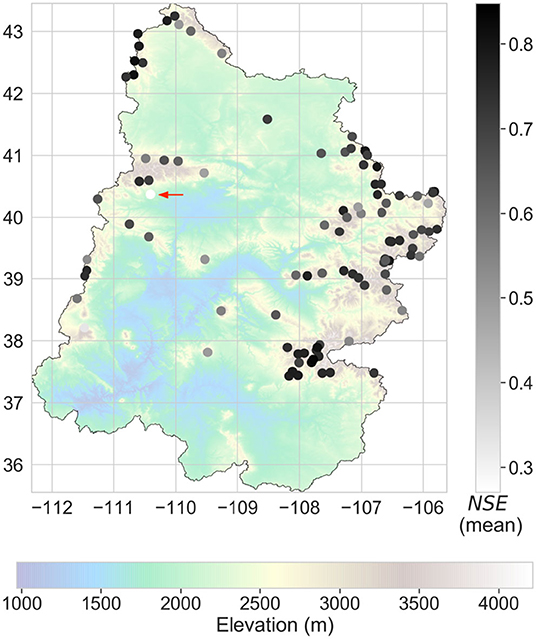
Figure 15. Geospatial distribution of mean NSE (μ_s) with a red arrow marking a station that has a low NSE.

Figure 6 shows sample scatter plots of true and predicted precipitation on test data using baseline imputations. We see from these plots that for a high value of NSE, the relative scatter is smaller. In addition, we can also observe that even for a high value of NSE, there is a tendency to overpredict the number of dry days and underestimate the intensity of extreme wet events. For subfigure (a), the 95th percentile threshold is at 15.24 mm, and for subfigure (b), it is at 12.7 mm. Recall that we define events beyond the 95th percentile threshold as extreme wet events.

Figures 8–11 demonstrate the benefits of sequential imputations when compared with non-sequential imputations. In what follows, we will use the phrase “incomplete station” to refer to an artificially incomplete station. Figures 8–11 show that as the proportion of incomplete stations increases, there is a higher percentage of stations benefitting from sequential imputation. ΔNSE values that correspond to significant improvements (i.e., Δ_sNSE > σ_s) tend to be higher than those that do not. A value of ΔNSE that does not correspond to a significant improvement (i.e., Δ_sNSE ≤ σ_s) implies that the previously imputed stations do not add extra information for spatial interpolation. This can be for two reasons: (i) the previously imputed stations are weakly correlated to the target station, or (ii) the previously imputed stations show strong correlations with the target station, but also show strong correlations with stations already in the complete subset. The second reason could happen if there is a cluster of stations that have similar physiography and experience similar precipitation patterns. Sequential imputation of stations in a cluster may not add new information if other stations in the cluster already have complete records. For instance, consider Scenario 4 where the proportion of incomplete stations is small and sequential imputation does not provide any benefits. Figure 4D shows that the incomplete stations in Scenario 4 are either isolated (and could be weakly correlated to other incomplete stations) or are a part of a cluster with multiple complete records. Figures 3, 4 show that the stations in our dataset tend to form clusters; these figures help us understand why we observe a smaller percentage of stations benefitting from sequential imputation as the proportion of incomplete stations decreases. The clustering tendency implies that when there is a small subset of incomplete stations, there is a high probability that previously imputed stations do not add any extra information for spatial information.

Figure 12 shows scatter plots of true and predicted precipitation on test data for a station that showed significant improvement during sequential imputation in Scenario 1. As noted for Figure 6 as well, these plots help visualize that as the NSE value increases during sequential imputation, the relative scatter decreases demonstrating improved spatial interpolation. Figures 13, 14 demonstrate that the benefits of sequential imputation also carry over to predicting dry events and extreme events despite the underlying limitations of spatial interpolation as noted in the section Evaluating Imputation: Nash Sutcliffe Efficiency (NSE). We observe a general trend that the improvements (or values of Δ) tend to be higher for stations that correspond to significant overall improvements (i.e., Δ_sNSE > σ_s) as discussed above.

Results for aggregate correlations (Figure 7B) show that the correlation between S_i (i.e., partial sum of first i sorted correlations) and NSE is high for lower values of i, and gets progressively weaker as i increases. This implies that for reliable imputation, having a few references that are strongly correlated is more important than having many references that are weakly correlated. This highlights why sequential imputation is a powerful technique, since leveraging even one incomplete station that is highly correlated to the target station can make a significant improvement. We illustrate this further in Figure 16, where we show values of S₂ for all stations at the time of sequential imputation in Scenarios 1 and 2. As expected, values of S₂ during sequential imputation are higher than those during non-sequential imputation, which is consistent with improved imputations.

FIGURE 16

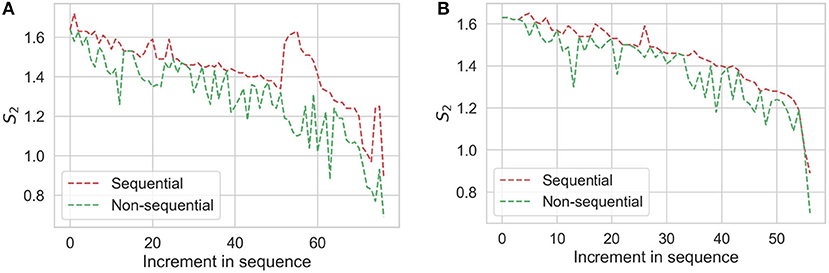
Figure 16. Comparisons between S₂ for sequential and non-sequential imputations: (A) Scenario 1 and (B) Scenario 2.

It is important to note that stations imputed earlier during sequential imputation tend to have a higher NSE, indicating a more reliable imputation. NSE values tend to decrease along the imputation sequence. This is primarily a consequence of the order in which we pick stations for sequential imputation. Stations that are imputed earlier in the sequence have a higher aggregate correlation with reference datasets, implying that missing data would be modeled with greater accuracy. This can be verified by observing the trend of the baseline NSE curve in Figures 8A–11A, which also shows a reduction in NSE values along the imputation sequence. Stations that are imputed later in the sequence will tend to have a lower value of NSE because they have a lower baseline NSE to begin with; they could still exhibit significant improvements during sequential imputation when compared to non-sequential imputation (as shown in Figures 8B–10B).

Finally, we note that the performance of sequential imputation could be negatively impacted if the data gaps among stations occur synchronously. In particular, this could happen if a station earlier in the sequence was poorly imputed and has a high correlation with a station imputed later in the sequence. However, the proposed sequential approach can still be implemented, and this approach will outperform or equally match the non-sequential approach.

Conclusions

Spatial interpolation algorithms typically require reference stations that have complete records; therefore, stations with missing data or incomplete records are not used. This limitation is critical for machine learning algorithms where incomplete records preclude data-driven learning of multi-variate relationships. In this study, we proposed a new algorithm, called the sequential imputation algorithm, for imputing missing time-series precipitation data. We hypothesized that stations with incomplete records contain information that can be used toward improving spatial interpolation. We confirmed this hypothesis by using the sequential imputation algorithm which was incorporated within a spatial interpolation method based on Random Forests.

We demonstrated the benefits of sequential imputation as compared to non-sequential imputation. Specifically, we showed that sequential imputation helps leverage other incomplete records for more reliable imputation. We observed that as the proportion of stations with incomplete records increases, there is a higher percentage of stations benefitting from sequential imputation. On the other hand, if the proportion of stations with incomplete records is small, there is a high probability that sequential imputation does not add any extra information for spatial information. We also observed that the benefits of sequential imputation carry over to improved predictions of dry events and extreme events. Finally, results showed that for reliable imputation, having a few strongly correlated references is more important than having many references that are weakly correlated. This highlights why sequential imputation is a powerful technique, since including even one incomplete station that is highly correlated to the target station can make a significant improvement in imputation.

Although we demonstrated sequential imputation using Random Forests, it can be implemented using other ML-based and spatial interpolation methods found in the literature. Furthermore, we presented a new but generic algorithm for imputing missing records in daily precipitation time-series that is potentially applicable to other meteorological variables as well.

Data Availability Statement

Publicly available datasets were analyzed in this study. This data can be found here: https://www.wcc.nrcs.usda.gov.

Author Contributions

UM and DD conceived and designed the study. UM acquired the data, developed the new algorithm, conducted all the numerical experiments, and analyzed the results. DD and JB provided input on methods and statistical analysis. BF provided input on data acquisition and time series analysis. DD helped analyze the results. SP and CS provided input on the conception of the study and were in charge of overall direction and planning. UM took the lead in writing the manuscript. All authors provided critical feedback and helped shape the research, analysis, and manuscript.

Funding

This work was funded by the ExaSheds project, which was supported by the U.S. Department of Energy, Office of Science, Office of Biological and Environmental Research, Earth and Environmental Systems Sciences Division, Data Management Program, under Award Number DE-AC02-05CH11231.

Conflict of Interest

The authors declare that the research was conducted in the absence of any commercial or financial relationships that could be construed as a potential conflict of interest.

Footnote

1. ^https://www.wcc.nrcs.usda.gov

References

Acock, M. C., and Pachepsky, Y. A. (2000). Estimating missing weather data for agricultural simulations using group method of data handling. J. Appl. Meteorol. 39, 1176–1184. doi: 10.1175/1520-0450(2000)039<1176:EMWDFA>2.0.CO;2

CrossRef Full Text | Google Scholar

Adhikari, R., and Agrawal, R. K. (2013). An Introductory Study on Time Series Modeling and Forecasting. Saarbrücken: LAP LAMBERT Academic Publishing.

Google Scholar

Ahmad, M. W., Mourshed, M., and Rezgui, Y. (2017). Trees vs. neurons: comparison between random forest and ANN for high-resolution prediction of building energy consumption. Energy Build. 147, 77–89. doi: 10.1016/j.enbuild.2017.04.038

CrossRef Full Text | Google Scholar

Box, G. E., and Jenkins, G. M. (1976). Time Series Analysis. Forecasting and control. Holden-Day Series in Time Series Analysis. San Francisco, CA: Holden-Day.

PubMed Abstract

Breiman, L. (2001). Random forests. Mach. Learn. 45, 5–32. doi: 10.1023/A:1010933404324

CrossRef Full Text | Google Scholar

Chen, L., Xu, J., Wang, G., and Shen, Z. (2019). Comparison of the multiple imputation approaches for imputing rainfall data series and their applications to watershed models. J. Hydrol. 572, 449–460. doi: 10.1016/j.jhydrol.2019.03.025

CrossRef Full Text | Google Scholar

Chuan, Z. L., Deni, S. M., Fam, S.-F., and Ismail, N. (2019). The effectiveness of a probabilistic principal component analysis model and expectation maximisation algorithm in treating missing daily rainfall data. Asia-Pac. J. Atmos. Sci. 56, 119–129. doi: 10.1007/s13143-019-00135-8

CrossRef Full Text | Google Scholar

Coulibaly, P., and Evora, N. D. (2007). Comparison of neural network methods for infilling missing daily weather records. J. Hydrol. 341, 27–41. doi: 10.1016/j.jhydrol.2007.04.020

CrossRef Full Text | Google Scholar

Daly, C., Halbleib, M., Smith, J. I., Gibson, W. P., Doggett, M. K., Taylor, G. H., et al. (2008). Physiographically sensitive mapping of climatological temperature and precipitation across the conterminous United States. Int. J. Climatol. 28, 2031–2064. doi: 10.1002/joc.1688

CrossRef Full Text | Google Scholar

Devi, G. K., Ganasri, B. P., and Dwarakish, G. S. (2015). A review on hydrological models. Aquat. Proced. 4, 1001–1007. doi: 10.1016/j.aqpro.2015.02.126

CrossRef Full Text | Google Scholar

Dwivedi, D., Arora, B., Steefel, C. I., Dafflon, B., and Versteeg, R. (2018). Hot spots and hot moments of nitrogen in a riparian corridor. Water Resour. Res. 54, 205–222. doi: 10.1002/2017WR022346

CrossRef Full Text | Google Scholar

Dwivedi, D., Steefel, I. C., Arora, B., and Bisht, G. (2017). Impact of intra-meander hyporheic flow on nitrogen cycling. Proced. Earth Planet. Sci. 17, 404–407. doi: 10.1016/j.proeps.2016.12.102

CrossRef Full Text | Google Scholar

Gao, Y., Merz, C., Lischeid, G., and Schneider, M. (2018). A review on missing hydrological data processing. Environ. Earth Sci. 77:47. doi: 10.1007/s12665-018-7228-6

CrossRef Full Text | Google Scholar

Gorshenin, A., Lebedeva, M., Lukina, S., and Yakovleva, A. (2019). “Application of machine learning algorithms to handle missing values in precipitation data,” in Distributed Computer and Communication Networks, eds V. M. Vishnevskiy, K. E. Samouylov, and D. V. Kozyrev (Cham: Springer International Publishing), 563–577.

Google Scholar

Gupta, H. V., Kling, H., Yilmaz, K. K., and Martinez, G. F. (2009). Decomposition of the mean squared error and NSE performance criteria: implications for improving hydrological modelling. J. Hydrol. 377, 80–91. doi: 10.1016/j.jhydrol.2009.08.003

CrossRef Full Text | Google Scholar

Hasanpour Kashani, M., and Dinpashoh, Y. (2012). Evaluation of efficiency of different estimation methods for missing climatological data. Stoch. Environ. Res. Risk Assess. 26, 59–71. doi: 10.1007/s00477-011-0536-y

CrossRef Full Text | Google Scholar

Hertig, E., Maraun, D., Bartholy, J., Pongracz, R., Vrac, M., Mares, I., et al. (2019). Comparison of statistical downscaling methods with respect to extreme events over Europe: validation results from the perfect predictor experiment of the COST Action VALUE. Int. J. Climatol. 39, 3846–3867. doi: 10.1002/joc.5469

CrossRef Full Text | Google Scholar

Hubbard, S. S., Varadharajan, C., Wu, Y., Wainwright, H., and Dwivedi, D. (2020). Emerging technologies and radical collaboration to advance predictive understanding of watershed hydro-biogeochemistry. Hydrol. Process. 34, 3175–3182. doi: 10.1002/hyp.13807

CrossRef Full Text | Google Scholar

Hubbard, S. S., Williams, K. H., Agarwal, D., Banfield, J., Beller, H., Bouskill, N., et al. (2018). The East River, Colorado, Watershed: a mountainous community testbed for improving predictive understanding of multiscale hydrological–biogeochemical dynamics. Vadose Zone J. 17, 1–25. doi: 10.2136/vzj2018.03.0061

CrossRef Full Text | Google Scholar

Jahan, F., Sinha, N. C., Rahman, M. M., Rahman, M. M., Mondal, M., and Islam, M. A. (2019). Comparison of missing value estimation techniques in rainfall data of Bangladesh. Theor. Appl. Climatol. 136, 1115–1131. doi: 10.1007/s00704-018-2537-y

CrossRef Full Text | Google Scholar

Kim, J.-W., and Pachepsky, Y. A. (2010). Reconstructing missing daily precipitation data using regression trees and artificial neural networks for SWAT streamflow simulation. J. Hydrol. 394, 305–314. doi: 10.1016/j.jhydrol.2010.09.005

CrossRef Full Text | Google Scholar

Lo Presti, R., Barca, E., and Passarella, G. (2010). A methodology for treating missing data applied to daily rainfall data in the Candelaro River Basin (Italy). Environ. Monit. Assess. 160, 1–22. doi: 10.1007/s10661-008-0653-3

PubMed Abstract | CrossRef Full Text | Google Scholar

Londhe, S., Dixit, P., Shah, S., and Narkhede, S. (2015). Infilling of missing daily rainfall records using artificial neural network. ISH J. Hydraul. Eng. 21, 255–264. doi: 10.1080/09715010.2015.1016126

CrossRef Full Text | Google Scholar

Louppe, G. (2015). Understanding random forests: from theory to practice (Ph.D. dissertation). University of Liège, Liège, Belgium.

Google Scholar

Morales Martínez, J. L., Horta -Rangel, F. A., Segovia-Domínguez, I., Robles Morua, A., and Hernández, J. H. (2019). Analysis of a new spatial interpolation weighting method to estimate missing data applied to rainfall records. Atmósfera 32, 237–259. doi: 10.20937/ATM.2019.32.03.06

CrossRef Full Text | Google Scholar

Moriasi, D. N., Arnold, J. G., Liew, M. W. V., Bingner, R. L., Harmel, R. D., and Veith, T. L. (2007). Model evaluation guidelines for systematic quantification of accuracy in watershed simulations. Trans. ASABE 50, 885–900. doi: 10.13031/2013.23153

CrossRef Full Text | Google Scholar

Oliver, M. A., and Webster, R. (2015). Basic Steps in Geostatistics: The Variogram and Kriging. Cham: SpringerBriefs in Agriculture, Springer International Publishing.

Google Scholar

Paulhus, J. L. H., and Kohler, M. A. (1952). Interpolation of missing precipitation records. Mon. Weather Rev. 80, 129–133.

Google Scholar

Pedregosa, F., Varoquaux, G., Gramfort, A., Michel, V., Thirion, B., Grisel, O., et al. (2011). Scikit-learn: machine learning in Python. J. Mach. Learn. Res. 12, 2825–2830.

Google Scholar

Ramos-Calzado, P., Gómez-Camacho, J., Pérez-Bernal, F., and Pita-López, M. F. (2008). A novel approach to precipitation series completion in climatological datasets: application to Andalusia. Int. J. Climatol. 28, 1525–1534. doi: 10.1002/joc.1657

CrossRef Full Text | Google Scholar

Schafer, J. L., and Graham, J. W. (2002). Missing data: our view of the state of the art. Psychol. Methods 7, 147–177. doi: 10.1037/1082-989X.7.2.147

PubMed Abstract | CrossRef Full Text | Google Scholar

Schneider, T. (2001). Analysis of incomplete climate data: estimation of mean values and covariance matrices and imputation of missing values. J. Clim. 14, 853–871. doi: 10.1175/1520-0442(2001)014<0853:AOICDE>2.0.CO;2

CrossRef Full Text | Google Scholar

Segal, M. R. (2004). Machine learning benchmarks and random forest regression. UCSF Center Bioinform. Mol. Biostat. 15. Available online at: https://archive.ics.uci.edu/ml/about.html

Google Scholar

Shepard, D. (1968). “A two-dimensional interpolation function for irregularly-spaced data,” in Proceedings of the 1968 23rd ACM National Conference (New York City, NY: ACM Press), 517–524.

Google Scholar

Simolo, C., Brunetti, M., Maugeri, M., and Nanni, T. (2010). Improving estimation of missing values in daily precipitation series by a probability density function-preserving approach. Int. J. Climatol. 30, 1564–1576. doi: 10.1002/joc.1992

CrossRef Full Text | Google Scholar

Stockman, M., Dwivedi, D., Gentz, R., and Peisert, S. (2019). Detecting control system misbehavior by fingerprinting programmable logic controller functionality. Int. J. Crit. Infrastruct. Prot. 26:100306. doi: 10.1016/j.ijcip.2019.100306

CrossRef Full Text | Google Scholar

Tang, F., and Ishwaran, H. (2017). Random forest missing data algorithms. Stat. Anal. Data Min. ASA Data Sci. J. 10, 363–377. doi: 10.1002/sam.11348

PubMed Abstract | CrossRef Full Text | Google Scholar

Teegavarapu, R. S. V. (2020). Precipitation imputation with probability space-based weighting methods. J. Hydrol. 581:124447. doi: 10.1016/j.jhydrol.2019.124447

CrossRef Full Text | Google Scholar

Teegavarapu, R. S. V., and Chandramouli, V. (2005). Improved weighting methods, deterministic and stochastic data-driven models for estimation of missing precipitation records. J. Hydrol. 312, 191–206. doi: 10.1016/j.jhydrol.2005.02.015

CrossRef Full Text | Google Scholar

Varadharajan, C., Faybishenko, B., Henderson, A., Henderson, M., Hendrix, V. C., Hubbard, S. S., et al. (2019). Challenges in building an end-to-end system for acquisition, management, and integration of diverse data from sensor networks in watersheds: lessons from a mountainous community observatory in East River, Colorado. IEEE Access 7, 182796–182813. doi: 10.1109/ACCESS.2019.2957793

CrossRef Full Text | Google Scholar

Yozgatligil, C., Aslan, S., Iyigun, C., and Batmaz, I. (2013). Comparison of missing value imputation methods in time series: the case of Turkish meteorological data. Theor. Appl. Climatol. 112, 143–167. doi: 10.1007/s00704-012-0723-x

CrossRef Full Text | Google Scholar

Zachara, J. M., Chen, X., Song, X., Shuai, P., Murray, C., and Resch, C. T. (2020). Kilometer-scale hydrologic exchange flows in a gravel bed river corridor and their implications to solute migration. Water Resour. Res. 56:e2019WR025258. doi: 10.1029/2019WR025258

CrossRef Full Text | Google Scholar

Zhai, P., Zhang, X., Wan, H., and Pan, X. (2005). Trends in total precipitation and frequency of daily precipitation extremes over China. J. Clim. 18, 1096–1108. doi: 10.1175/JCLI-3318.1

CrossRef Full Text | Google Scholar