Abstract
3D morphable models are widely used to describe the variation of human body shapes. However, these models typically focus on the surface of the human body, since the acquisition of the volumetric interior would require prohibitive medical imaging. In this paper we present a novel approach for creating a volumetric body template and for fitting this template to the surface scan of a person in a just a few seconds. The body model is composed of three surface layers for bones, muscles, and skin, which enclose the volumetric muscle and fat tissue in between them. Our approach includes a data-driven method for estimating the amount of muscle mass and fat mass from a surface scan, which provides more accurate fits to the variety of human body shapes compared to previous approaches. We also show how to efficiently embed fine-scale anatomical details, such as high resolution skeleton and muscle models, into the layered fit of a person. Our model can be used for physical simulation, statistical analysis, and anatomical visualization in computer animation and medical applications, which we demonstrate on several examples.
1 Introduction
Virtual humans are present in our everyday lives. They can be found in movies, computer games, and commercials. In addition, they are employed in a rapidly growing number of applications in virtual reality (VR) and augmented reality (AR), even ranging to computational medicine. All these applications benefit from realistic virtual representations of human.
If we look at a human, its appearance is mostly determined by everything we can directly see (skin, hair, cloth, etc.). Hence, it is not surprising that research has focused on capturing, analyzing, and animating surface models of humans. Consequently, there is a vast amount of surface-based capturing approaches, suitable for almost every level of detail and budget: From complex multi-camera photogrammetry setups that capture finest-scale wrinkles of the human face (Riviere et al., 2020) over approaches that compute ready-to-animate models from simple smart-phone videos (Wenninger et al., 2020) to machine learning approaches that reconstruct a virtual model from a single image (Weng et al., 2019). For the purpose of creating convincing animations of and interactions with those models, large amounts of 3D captured data have been collected to build sophisticated surface-based models (Anguelov et al., 2005; Loper et al., 2015; Bogo et al., 2017). Those models compensate for the fact that humans are not empty hulls or homogeneous solids by capturing and analyzing more and more data of that surface hull. Another way to approach this is to model volumetric virtual humans by incorporating (discrete approximations of) their interior anatomical structures. While surface-based models might be sufficient for many applications, for others (e.g., surgery simulation) a volumetric model is an essential prerequisite.
While detailed volumetric models of the human body exist (Ackerman, 1998; Christ et al., 2009; Zygote, 2020), they can be very tedious to work with. Since they usually consist of hundreds of different bones and muscles, merely creating a volumetric tetrahedral mesh for simulation purposes can be frustratingly difficult. Moreover, those models represent average humans and transferring their volumetric structure and anatomical details to a specific human model (e.g., a scanned person) is not straightforward. Although there are a couple of approaches for transferring the interior anatomy from a volumetric template model into a surface-based virtual human (Dicko et al., 2013; Kadleček et al., 2016), these methods either deform bone structures in a non-plausible manner (Dicko et al., 2013) or require a complex numerical optimization (Kadleček et al., 2016).
In this paper we present a robust and efficient method for transferring an interior anatomy template into a surface mesh in just a couple of seconds. A key component is a simple decomposition of the human body into three layers that are bounded by surfaces sharing the same triangulation: the skin surface defines the outer shape of the human, the muscle surface envelopes its individual muscles, and the skeleton surface wraps the subject’s skeleton (see Figure 1 middle). The muscle layer is hence enclosed in between the skeleton and muscle surface, and the subcutaneous fat tissue by the muscle surface and skin surface. This layered template model is derived from the Zygote body model (Zygote, 2020), which provides an accurate representation of both the male and female anatomy. We propose simple and fast methods for fitting the layered template to surface scans of humans and for transferring the high-resolution anatomical details (Zygote, 2020) into these fitted layers (see Figure 1 right). Our method is robust, efficient, and fully automatic, which we demonstrate on about 1,700 scans from the European CAESAR dataset (Robinette et al., 2002).
FIGURE 1
Our approach enriches simple surface scans by plausible anatomical details, which are suitable for educational visualizations and volumetric simulations. We note, however, that due to the lack of true volumetric information, it is not a replacement of volumetric imaging techniques in a medical context. Our main contributions are:
• A novel approach for creating a layered volumetric template defined by skin, muscle, and bone surfaces, which all have the same triangulation, thereby making volumetric tessellation straightforward.
• A robust and efficient method for transferring the layered volumetric template model into a given surface scan of a human in just a couple of seconds.
• A regressor that extracts the amount of muscle and fat mass of a subject from the skin surface only, thereby making manual specification of muscle and fat distribution unnecessary.
• Our approach takes differences between male and female anatomy into account by deriving individual volumetric templates and individual muscle/fat regressors for men and women.
2 Related Work
Using a layered volumetric model of a virtual character has been shown beneficial compared to a surface-only model in multiple previous works. Deul and Bender (2013) compute a simple layered model representing a bone, muscle, and fat layer, which they use for a multi-layered skinning approach. Simplistic layered models have also been used to extend the SMPL surface model (Loper et al., 2015) in order to support elastic effects in skinning animations (Kim et al., 2017; Romero et al., 2020). Compared to these works, our three layers yield an anatomically more accurate representation of the human body, while still being simpler and more efficient than complex irregular tetrahedralizations. Saito et al. (2015) show that a layer that envelopes muscles yields more convincing muscle growth simulations and reduces the number of tetrahedral elements required in their computational model. They also show how to simulate different variations of bone sizes, muscle mass and fat mass for a virtual character.
When it comes to the generation of realistic personalized anatomical structures from a given skin surface, most previous works focus on the human head: Ichim et al. (2016) register a template skull model to a surface-scan of the head in order to build a combined animation model using both physics-based and blendshape-based face animation. Ichim et al. (2017) also incorporate facial muscles and a muscle activation model to allow more advanced face animation effects. Gietzen et al. (2019), Achenbach et al. (2018) use volumetric CT head scans and surface-based head scans in order to learn a combined statistical model of the head surface, the skull surface, and the enclosed soft tissue, which allows them to estimate the head surface from the skull shape and vice versa. Regarding the other parts of the body, Zhu et al. (2015) propose an anatomical model of the upper and lower limbs that can be fit to surface scans and is able to reconstruct motions of the limbs.
To our knowledge, there are just two former approaches for generating an anatomical model of the complete core human body (torso, arms, legs) from a given skin surface. In their pioneering work, Dicko et al. (2013) transfer the anatomic details from a template model to various humanoid target models, ranging from realistic body shapes to stylized non-human characters. They transfer the template’s anatomy through a harmonic space warp and per-bone affine transformations, which, however, might distort muscles and bones in an implausible way. Different distributions of subcutaneous fat can be (and have to be) painted manually into a special fat texture. The work of Kadleček et al. (2016) is most closely related to our approach. They build an anatomically plausible volumetric model from a set of 3D scans of a person in different poses. An inverse physics simulation is used to fit a volumetric anatomical template model to the set of surface scans, where custom constraints prevent muscles and bones from deforming in an unnatural manner. We discuss the main differences of our approach and Dicko et al. (2013), Kadleček et al. (2016) in Section 4.
Estimating the body composition from surface measures or 3D surface scans (like we do in Section 3.3) has been tackled before. There are numerous formulas for computing body fat percentage (BF), or body composition in general, from certain circumferences, skinfold thicknesses, age, gender, height, weight, and density measurements. Prominent examples are the skinfold equations, or the Siri- and Brozek formulas (Siri, 1956; Brožek et al., 1963; Jackson and Pollock, 1985). These formulas, however, either rely on anthropometric measurements that have to be taken by skilled personnel or on measuring the precise body density via expensive devices, such as BOD PODs (Fields et al., 2002). Ng et al. (2016) compute BF based on a 3D body scan of the subject, but their formula is tailored toward body scans and measurements taken with the Fit3D Scanner (Fit3D, 2021). Even with the help of the authors we could not successfully apply their formulas to scans taken with different systems, since we could always find examples resulting in obviously wrong (or even negative) BF. Recently, Maalin et al. (2020) showed that modeling body composition through body fat alone is an inferior measure for defining the shape of a person compared to a combined model of fat mass and muscle mass. We therefore adapt their data to estimate fat mass and muscle mass from surface scans alone (Section 3.3). Incorporating these estimations into the volumetric fitting process allows us to determine how much of the soft tissue layer is described by muscle tissue more plausibly than Kadleček et al. (2016).
3 Methods
Our approach consists of three main contributions: First, the generation of the volumetric three-layer template, described in Section 3.2, where we derive the skin, muscle, and skeleton layers from the male and female Zygote model (Zygote, 2020). Second, an efficient method for fitting this layered model (including all contained anatomical details) (in)to a given human surface scan (Section 3.4). Third, the estimation of a person’s body composition, i.e., how much of the person’s soft tissue is described by muscles and fat (Section 3.3). By adapting the BeyondBMI dataset (Maalin et al., 2020) to our template, we derive this information from the surface scan alone and use it to inform the volumetric template fitting. Figure 2 shows an overview of the whole process, starting from the different input data sets, the template model and the muscle/fat regressor, to the final personalized anatomical fit.
FIGURE 2
3.1 Data Preparation
In our approach we make use of several publicly or commercially available datasets for model generation, model learning, and evaluation:
• Zygote: The Zygote model (Zygote, 2020) provides high-resolution models for the male and female anatomy. We use their skin, muscle, and skeleton models for building our layered template.
• BeyondBMI: Maalin et al. (2020) scanned about 400 people and additionally measured their fat mass (FM), muscle mass (MM), and body mass index (BMI) using a medical-grade eight-electrode bioelectrical impedance analysis. They provide annotated (synthetic) scans of 100 men and 100 women, each computed by averaging shape and annotations of two randomly chosen subjects. From this data we learn a regressor that estimates fat and muscle mass from the skin surface.
• Hasler: The dataset of Hasler et al. (2009) contains scans of 114 subjects in 35 different poses, captured by a 3D laser scanner. The scans are annotated with fat and muscle mass percentage as measured by a consumer-grade impedance spectroscopy body fat scale. We use this dataset to evaluate the regressor learned from the BeyondBMI data.
• CAESAR: The European subset of the CAESAR scan database (Robinette et al., 2002) consists of 3D scans (with about 70 selected landmarks) equipped with annotations (e.g., weight, height, BMI) of about 1,700 subjects in a standing pose. We use this data to evaluate our overall fitting procedure.
All these data sources use different model representations, i.e., either different mesh tessellations or even just point clouds. In a preprocessing step we therefore re-topologize the skin surfaces of these datasets to a common triangulation by fitting a surface template using the non-rigid surface-based registration of Achenbach et al. (2017).
This approach is based on an animation-ready, fully rigged, statistical template model. Its mesh tessellation (about 21k vertices), animation skeleton, and skinning weights come from the Autodesk Character Generator (Autodesk, 2014). It uses a 10-dimensional PCA model representing the human body shape variation and we will call it the surface template in the following. In a preprocessing step we fit the surface template to all input surface scans to achieve a common triangulation and thereby establish dense correspondence. This fitting process is guided by a set of landmarks, which are either specified manually or provided by the dataset. A nonlinear optimization then determines alignment (scaling, rotation, translation), body shape (PCA parameters), and pose (inverse kinematics on joint angles) in order to minimize squared distances of user-selected landmarks and automatically determined closest point correspondences in a non-rigid ICP manner (Bouaziz et al., 2014b). Once the model parameters are optimized, a fine-scale out-of-model deformation improves the matching accuracy and results in the final template fit. For more details we refer to (Achenbach et al., 2017).
3.2 Generating the Volumetric Template
We use the male and female Zygote body model (Zygote, 2020) as a starting point for our volumetric model. Our volumetric template is defined by the skeleton surface (for bones), the muscle surface, and the skin surface. The skeleton is enveloped by the skeleton surface, the muscle layer is enclosed between the skeleton surface and the muscle surface, and the (subcutaneous) fat layer is enclosed by the muscle surface and the skin surface. The soft-tissue layer is the union of the fat and muscle layers. In our layered model we exclude the head, hands, and toes. These regions will be identical to the skin surface in all layers. See Figure 3 for a visualization of the layered template.
FIGURE 3
The three surfaces , , and will be constructed to share the same triangulation, providing a straightforward one-to-one correspondence between the ith vertices on each surface, which we denote by , , and , respectively. Each two corresponding triangles on and on span a volumetric element of the fat layer. Similarly, the volumetric elements of the muscle layer are spanned by pairs of triangles on and on . We call these elements, built from six vertices of two triangles, prisms, and will either use them directly in a simulation or (trivially) split them into three tetrahedra each, resulting in a simple conforming volumetric tessellation.
The following two sections describe how to generate the skeleton surface (Section 3.2.1) and the muscle surface (Section 3.2.2). The skin surface is generated by fitting the surface-based template of Achenbach et al. (2017) to the skin of the anatomical model (Zygote, 2020), as described in Section 3.1.
3.2.1 The Skeleton Surface
The skeleton surface should enclose all the bones of the detailed skeleton model, as shown in Figure 3, center. We achieve this by shrink-wrapping the skin surface onto the skeletal bones. To avoid problems caused by gaps between bones (e.g., rib-cage, tibia/fibula), we first generate a skeleton wrap , a watertight genus-0 surface that encapsulates the bones, and then shrink-wrap the skin surface to instead. The wrap surface can easily be generated by a few iterations of shrink-wrapping, remeshing, and smoothing of a bounding sphere in a 3D modeling software like Blender or Maya. This results in a smooth, watertight, and two-manifold surface that excludes regions like the interior of the rib-cage and small holes like in the pelvis or between ulna and radius.
We generate the skeleton surface by starting from the skin surface , i.e., setting , and then minimizing a nonlinear least squares energy that is composed of a fitting term, which attracts the surface to the bone wrap , and a regularization term, which prevents from deforming in a physically implausible manner from its initial state :The regularization is formulated as a discrete bending energy that penalizes the change of mean curvature, measured as the change of length of the Laplacian:where and denote the vertex positions of the deformed surface and the initial surface , respectively. The matrix denotes the optimal rotation aligning the vertex Laplacians and , which are discretized using the cotangent weights and the Voronoi areas (Botsch et al., 2010).
The fitting term penalizes the squared distance of vertices from their target positions :The target positions are points (not necessarily vertices) on the skeleton wrap of either one of three types: closest point correspondences, fixed correspondences, or collision targets. The weight is determined solely by the type of target position (0.1 for closest point correspondences, 1 for fixed correspondences, 100 for collision targets). We define just one target for each vertex . The default is a closest point correspondence per vertex, which can be overridden by a fixed correspondence, and both of them will be overridden by the collision target in case of a detected collision. Below we explain the three target types.
Closest point correspondences are updated in each iteration of the minimization to the closest position on to the vertex , i.e., .
Near complicated regions, like the armpit or the rib-cage, the skin has to stretch considerably to deform toward the skeleton wrap. As a consequence, corresponding triangles on the skin surface and on the eventual skeleton surface will not be approximately on top of each other, but instead be tangentially shifted. These two triangles span a volumetric element that we call a prism. Misaligned triangles will lead to heavily sheared prisms, which can cause artifacts in physical simulations.
We define a per-vertex score penalizing misalignment of corresponding vertices and w.r.t. their common averaged normal :A 2D example of this is shown on the right, where the closest correspondence of is . The position that maximizes the minimal angle at both vertices is , where the connecting line (dotted red) aligns with the average normal.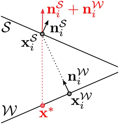
Fixed correspondences are responsible for reducing these tangential shifts and thereby improving the prism shapes. We determine them for some vertices at the beginning of the fit as explained in the following and keep them fixed throughout the optimization. Since the alignment error increases faster if the distance between skin surface and skeleton wrap is small, we specify fixed correspondences for vertices on that have a distance <3 cm to . For each such vertex we randomly sample points in the geodesic neighborhood of and select the one that minimizes Eq. 4 as fixed alignment constraint, where we generate normal vectors of sample points using barycentric Phong interpolation. To avoid interference of spatially close fixed correspondences, we add them in order of increasing distance to the skeleton, but only if their distance to all previously selected points is larger than 5 cm. In that way, we get a well distributed set of fixed correspondences, favoring those with a small skin-to-skeleton distance. Figure 4, center, shows that this already reduces the alignment error by a large amount.
FIGURE 4
Closest point correspondences can also drag vertices to locations with high alignment error. In each iteration of the nonrigid ICP, we compute for each vertex on and its counterpart on the current state of . If this error exceeds a limit of 0.01, which corresponds to an angle deviation of 8° from the optimal angle, we sample the one-ring neighborhood of vertex on and set to the sample with minimal alignment error and update its closest point correspondence on . This strategy reduces the alignment error even further, as shown in Figure 4, right.
In the process of moving the surface toward , these two meshes might intersect each other, violating our goal that in the converged state the surface [i.e., , due to (Eq. 1)] should fully enclose . We therefore detect these collisions during the optimization and resolve them through collision targets. We use the exact continuous collision detection of Brochu et al. (2012) to detect collisions. In case of a collision, we back-track the triangles’ linear path from the current to the initial to find the non-colliding state closest to . This state defines collision targets for colliding vertices , which override the other types of target positions. In case of multiple collision targets for the same vertex , we determine all non-colliding states separately and choose the one that is closest to the initial skin surface . Minimizing (Eq. 1) leads to the final skeleton surface (Figure 3B). See Appendix for more details about the optimization strategy.
3.2.2 The Muscle Surface
We generate the muscle surface by minimizing the same energy as in Eq. 1, but using a different method for finding the correspondences in Eq. 3, which exploits that we already established correspondence between skin surface and skeleton surface . We do not employ closest point correspondences, but instead set for each vertex a fixed correspondence to the first intersection of the line from skin vertex to skeleton vertex with the high-resolution muscle model (Zygote, 2020). If there is no intersection (e.g., at the knee), we set and assign a lower weight . When the minimization converges and we decrease , we project the vertices of the current muscle surface to their corresponding skin-to-skeleton line from to . Due to the collision handling, the resulting muscle surface will enclose the high-resolution muscle model. To ensure that our volumetric elements always have a non-zero volume, even in regions where there is no muscle between skin and bone, we ensure a minimal offset of 1 mm from to the skeleton mesh. The resulting muscle surface is visualized in Figure 3C. Note that the muscle layer does not exclusively contain muscles: Especially in the abdominal region, a large amount of the muscle layer is filled by organs. We therefore define a muscle thickness map that for each vertex i stores the accumulated length of the segments of the line () that are covered by muscles. This map will be used later in Section 3.4.3.
3.3 Estimating Fat Mass and Muscle Mass
Having generated the volumetric layered template, we want to be able to fit it to a given surface scan of a person. To regularize this under-determined problem, we first have to estimate how much of the person’s soft tissue is explained by fat mass (FM) and muscle mass (MM), respectively. This is a challenging problem since we want to capture a single surface scan of the person only and therefore cannot rely on information provided by additional hardware, such as a DXA scanner or a body fat scale. Kadleček et al. (2016) handle this problem by describing the person’s shape primarily through muscles, i.e., by growing muscles as much as possible and defining the remaining soft tissue volume as fat. This strategy results in adipose persons having considerably more muscle mass than leaner people. Although there is a certain correlation between total body mass (and also BMI) and muscle mass – because the higher weight has a training effect especially on the muscles of the lower limbs (Tomlinson et al., 2016) – this general trend is not sufficient to define the body composition of people.
Maalin et al. (2020) measured both FM and MM using a medical-grade eight-electrode bio-electrical impedance analysis and acquired a 3D surface scan. From this data, they built a model that can vary the shape of a person based on specified muscle or fat variation, similar to Piryankova et al. (2014). Our model should perform the inverse operation, i.e., estimate FM and MM from a given surface scan. We train our model on their BeyondBMI dataset (Section 3.1), which consists of scans of 100 men and 100 women captured in an approximate A-pose (see Figure 5), each annotated with FM, MM, and BMI.
FIGURE 5
By applying the surface fitting described in Section 3.1 to the BeyondBMI dataset, we make their scans compatible to our template and un-pose their scans to a common T-pose, thereby making any subsequent statistical analysis pose-invariant. After re-excluding the head, hands, and feet of our surface template, we are left with meshes per sex that consist of vertices . We denote the training mesh by a -dimensional vector of stacked vertex coordinatesand perform PCA on the data matrix . Let be the basis of the subspace spanned by the first k principal components and the mean of the training data. Since the data is now pose-normalized, the dimensionality reduction can focus solely on differences in human body shape. As a result, our model only needs PCA components to explain 99.5% of the data variance, while the original BeyondBMI dataset needs components to cover the same percentage due to noticeable variations in pose during the scanning process (see Figure 5). We then perform linear regression to estimate FM and MM from PCA weights, as proposed by Hasler et al. (2009).
For a first evaluation of this model, we perform a leave-one-out test on the BeyondBMI dataset, i.e., excluding each scan once, building the regressors as described above from the remaining scans, and measuring the mean absolute error of the predictions. We again use PCA components, as this covers almost all the variance present in the dataset and gives the linear regression enough degrees of freedom. The leave-one-out evaluation yields a mean absolute error (MAE) of and for the female dataset, where the fat mass lies in the range 6.27–34.71 kg and the muscle mass in the range 21.59–31.63 kg. The linear regression shows an average score of 0.84, confirming that there is indeed a linear relationship between PCA coordinates and the FM/MM measurements. Performing the leave-one-out test on the male dataset shows similar values: and , fat mass in the range 3.91–27.83 kg, muscle mass in the range 31.51–51.20 kg, and an average score of 0.88.
We compared the linear model to a support vector regression (using scikit-learn (Pedregosa et al., 2011) with default parameters and RBF kernels), but in contrast to Hasler et al. (2009) we found that for the BeyondBMI dataset this approach performs considerably worse: and with an average score of 0.64 for the female dataset, and and with an average score of 0.58 for the male dataset. We therefore keep the simpler and better-performing linear regression model.
Whenever we fit the volumetric model to a given body scan, as explained in the next section, we first use the proposed linear regressors to estimate the person’s fat mass and muscle mass and use this information to generate the muscle and fat layers in Section 3.4.3.
3.4 Fitting the Volumetric Template to Surface Scans
Given a surface scan, we transfer the template anatomy into it through the following steps: First, we fit our surface template to the scan, which establishes one-to-one correspondence with the volumetric template and puts the scan into the same T-pose as the template (Section 3.1). After this pre-processing, we deform the volumetric template to match the scanned subject. To this end, we adjust global scaling and per-bone local scaling, such that body height and limb lengths of template and scan match (Section 3.4.1). This is followed by a quasi-static deformation of the volumetric template that considers the skin surface as hard constraint and yields the skeleton surface through energy minimization (Section 3.4.2). Given the skin surface , the bone surface , and the estimated fat mass and muscle mass from Section 3.3, the muscle surface is determined (Section 3.4.3). Having transferred all three layer surfaces to the scan we finally warp the detailed anatomical model to the target (Section 3.4.4).
3.4.1 Global and Local Scaling
Fitting the surface template to the scanner data puts the latter into the same alignment (rotation, translation) and the same pose as the volumetric template. The next step is to correct the mismatch in scale by adjusting body height and limb lengths of the volumetric template.
This scaling does influence all three of the template’s surfaces. Since the shape of the skeleton surface will be constrained to the result after scaling, we have to scale in a way that keeps bone lengths and bone diameters within a plausible range. The length of prominent bones, like the upper arm or the upper leg (humerus and femur), can be well approximated by measures on the surface of the model. But finding the correct bone diameters is impossible without measurements of the subject’s interior. In particular for corpulent or adipose subjects, the subcutaneous fat layer dominates the appearance of the skin surface, preventing us from precisely determining the bone diameters from the surface scan. It has been shown that there is a moderate correlation of bone length and bone diameter (Ziylan and Murshid, 2002; Aydin Kabakci et al., 2017) and (obviously) a strong correlation of body height and bone length (Dayal et al., 2008). We therefore perform a global isotropic scaling depending on body height (affecting bone lengths and diameters) as well as local anisotropic scaling depending on limb lengths (affecting bone lengths only).
The global scaling is determined from the height difference of scan and template and is applied to all vertices of the template model. It therefore scales all bone lengths and bone diameters uniformly. Directly scaling with the height ratio of scan and template, however, can result in bones too thin or too thick for extreme target heights. Thus, we damp the height ratio by , which means that a person that is 20% taller than the template will have 10% thicker bones than the template. This heuristic results in visually plausible bone diameters for all our scanned subjects.
After the global scaling, the local scaling further adjusts the limb lengths of the template to match those of the scan. The (fully rigged) surface-based template has been fit to both the scan (Section 3.1) and the template (Section 3.2). This fit provides a simple skeleton graph (used for skinning animation) for both models. We use the length mismatch of the respective skeleton graph segments to determine the required scaling for upper and lower arms, upper and lower legs, feet, and torso. We scale these limbs in their corresponding bone directions (or the spine direction for the torso) using the bone stretching of Kadleček et al. (2016). As mentioned before, this changes the limb lengths but not the bone diameters.
This two-step scaling process is visualized in Figure 6. As a result, the scaled template matches the scan with respect to alignment, pose, body height, and limb lengths. Its layer surfaces, which we denote by , , and , provide a good initialization for the optimization-based fitting described in the following.
FIGURE 6
3.4.2 Skeleton Fitting
Given the coarse registration of the previous step, we now fit the skin surface and skeleton surface by minimizing a quasi-static deformation energy. Since the template’s skin surface should match the (skin) surface of the scan and since both meshes have the same triangulation, we can simply copy the skin vertex positions from the scan to the template and consider them as hard Dirichlet constraints. It therefore remains to determine the vertex positions of the skeleton surface , such that the soft tissue enclosed between skin surface and skeleton surface (fat + muscles, which we call flesh) deforms in a physically plausible manner. This is achieved by minimizing a quasi-static energy consisting of three terms:The first term is responsible for keeping the skeleton surface (approximately) rigid and uses the same formulation as Eq. 2, with and denoting the skeleton surface before and after the deformation, respectively. We employ a soft constraint with high weight instead of deforming bones in a strictly rigid manner (Kadleček et al., 2016), since we noticed that for very thin subjects the skeleton surface might otherwise protrude the skin surface and therefore a certain amount of bone deformation is required. We also do not penalize deviation from rigid or affine transformations as Dicko et al. (2013) since this penalizes smooth shape deformation in the same way as locally flipped triangles, which we observed to cause artifacts in the skeleton surface. The discrete bending energy of Eq. 2, with a suitably high regularization weight , allows for moderate smooth deformations and gave better results in our experiment.
The second term prevents strong deformations of the prism elements , spanned by corresponding triangles on the skin surface and on the skeleton surface. While we penalize deformation of the top/bottom triangles, we allow changes of prism heights, i.e., anisotropic scaling in the direction from surface to bone, since otherwise the fat layer cannot grow to bridge the gap from the skeleton surface to the skin surface. This behavior is modeled by the anisotropic strain limiting energywhere is the deformation gradient of the element p, i.e., the linear part of the best affine transformation that maps the un-deformed prism to the deformed prim p in the least squares sense. If denotes the edge direction matrix of the prism p and the respective matrix of , then . Polar decomposition (Shoemake and Duff, 1992) decomposes into a rotation and scale/shear . is a rotation matrix that aligns the z-axis with the surface normal of the prism’s corresponding skin triangle, i.e., the direction in which we allow stretching. The matrix represents the anisotropic scaling , where allows to tune the amount of stretching in normal direction that should be allowed. We use and to allow stretching and compression of the element by a factor of five before the energy of this element increases.
Third, we detect all collisions , defined as vertices of the skeleton surface that are outside of the skin surface . For these colliding vertices we add a collision penalty termwhere is the projection of the colliding vertex to a position 2 mm beneath the closest triangle on the skin surface . The weight is defined per vertex, is set to 1 the first time a vertex is colliding, and is increased by 1 each time the minimization was not able to resolve the collision. The iterative minimization of (Eq. 5) as well as the computation of the individual elements of (Eq. 6) is further detailed in Appendix.
3.4.3 Muscle Fitting
Having determined the skin surface and skeleton surface , we now fit the muscle surface in between and , such that the ratio of fat mass (FM) and muscle mass (MM) resembles the values estimated by our regressors (Section 3.3). We proceed in three steps: First, we transfer the template’s muscle distribution to the fitted skin and skeleton surfaces, which we call average muscle layer in the following. Second, we grow and shrink the muscles as much as anatomically and physically plausible, yielding the minimum and maximum muscle layers. Third, we find a linear interpolation between these two extremes that matches the predicted fat mass and muscle mass as good as possible.
The average muscle surface is transferred from the scaled template (Section 3.4.1; Figure 6) by minimizing an energy consisting of two objectives:The first term tries to preserve the shape of the scaled template’s muscle surface and is modeled using the regularization energy of Eq. 2. The second term preserves the template’s property that each muscle vertex resides on the line segment from its corresponding skeleton vertex to its skin vertex , by penalizing the squared distance from that line:where is the projection of onto the line , . Minimizing 8) leads to flat abdominal muscles like in the template model, which is unrealistic for corpulent or adipose subjects, because the majority of body fat resides in two different fat tissues: the subcutaneous fat, which resides between skin and muscle surface, and the visceral fat, which accumulates in the abdominal cavity, i.e., under the muscle layer. Since the bulging of the abdomen due to visceral fat causes a bulging of the belly, we inversely want the abdominal muscles in to slightly bulge out in case of a belly bulge in the skin surface . The latter is a combined effect of visceral and subcutaneous fat in the abdominal region. We model this effect by adjusting for each vertex in the abdominal region. Instead of using the full interval , we adjust the lower boundary to , i.e., the parameter α where for the (scaled) template the muscle surface intersects the line. The iterative minimization of (Eq. 8) is further detailed in Appendix.
Having transferred the average muscle surface, we next grow/shrink muscles as much as possible in order to define the maximum/minimum muscle surfaces. Since certain muscle groups might be better developed than others, we perform the muscle growth/shrinkage separately for the major muscle groups, namely upper legs (including buttocks), lower legs, upper arms, lower arms, chest, abdominal muscles, shoulders, and back. Muscles are built from fibers and grow perpendicular to the fiber direction. In all cases relevant for us, the fibers are approximately perpendicular to the direction from to , thus muscle growth/shrinkage will move vertices along the line from to . The amount of vertex movement along these directions is proportional to the muscle thickness map of the template (computed in Section 3.2.2). We determine how much we can grow a muscle before it collides with the skin surface in the thicker parts of the muscle (instead of close to its endpoints where it connects to the bone). Figure 7 shows an example, where the leftmost muscle vertex is already close to the skin and would prevent any growth if we took endpoint regions into account. For each muscle group, we also define an upper limit for muscle growth that prevents the muscles from increasing further even if the skin distance is large (e.g., for adipose subjects). For determining the minimal muscle surface, we repeat the process in the opposite direction (toward the skeleton surface). To prevent distortions of the muscle surface, we do not set the new vertex positions directly, but instead use them as target positions (using Eq. 3) and regularize with Eq. 8. Figure 7 (right) shows an example of minimum/maximum muscle surfaces computed by this procedure.
FIGURE 7
We determine the final muscle surface by linear interpolation between the minimum and maximum muscle surfaces, such that the resulting fat mass FM and muscle mass MM match the values predicted by the regressors (denoted by and ) as good as possible. To this end we have to compute FM and MM from an interpolated muscle surface . We can compute the volume of the fat layer (between and ) and the volume of the muscle layer (between and ) and convert these to masses and by multiplying with the (approximate) fat and muscle densities and , respectively.
The resulting masses require some corrections though: First, we have to add the visceral fat (VAT), which is not part of our fat layer but resides in the abdominal cavity. We estimate the VAT mass by computing the difference of the cavity volumes of the scaled template and of the final fit, thereby assuming a negligible amount of VAT in the template. Second, we subtract the skin mass from the fat layer mass. We assume an average skin thickness of 2 mm, multiply this by the skin’s surface area and the density . Third, our fat layer includes the complete reproductive apparatus in the crotch region. This volume is even larger due to the underwear that was worn during scanning and incorrectly increases the fat layer mass by . Our corrected fat mass is thenWe correct the muscle mass by subtracting the mass of the abdominal cavity, which is incorrectly included in the muscle layer. The remaining muscle mass is always too small even when using the maximum muscle surface, due to all muscles not considered in the muscle layer, such as heart, face, and hand muscles or the diaphragm. It is known that the lean body mass roughly scales with the squared body height (Heymsfield et al., 2011), which is the basis of the well known body and muscle mass indices. We analogously assume the missing muscle mass to be proportional to the squared height h of the subject, i.e., , with a constant k to be determined later. The corrected muscle mass is thereforeThere are other terms like the fat of head, hands, and toes, which could be added, or the volume of blood vessels and tendons, which could be subtracted. We assume those terms to be negligible.
Since the total volume of the soft tissue layer is constant, the muscle layer mass is coupled to the fat layer mass via . We want to compute the fat layer mass such that the resulting FM and MM minimize the least squares error to the values predicted by the regressor: . Inserting (Eqs 10, 11) into E, rewriting in terms of , and setting the derivative yields the optimal fat layer masswith the density ratio
The minimum/maximum muscle surface yields a maximum/minimum fat layer mass. The optimized fat layer mass is clamped to meet this range, thereby defining the final fat layer mass. We then choose the linear interpolant between the minimum and maximum muscle surface that matches this fat mass, which we find through bisection search.
We did this for the scans of 100 men and 100 women from the BeyondBMI dataset (Maalin et al., 2020), where we know the true values for FM and MM from measurements, and optimized the value of k for this dataset, yielding and . This is plausible since women in general have a lower muscle mass. For instance, the average muscle mass of the male subjects in the dataset is indeed 50% higher than the average MM for the female subjects. The mean absolute errors (MAE) for the BeyondBMI dataset are , for the female subjects and , for the male subjects. Figure 8 shows how well our model can adjust to the target values of muscle and fat mass. All values are inside or at least close to the predicted possible range of minima and maxima. Moreover, in most cases the muscle/fat mass values for the same person split the two ranges at about an inverse point (e.g., close to maximum muscle and close to minimum fat), which leads to the low errors stated above.
FIGURE 8
3.4.4 Transferring Original Anatomical Data
After fitting the skin surface to the scan and transferring the skeleton surface and the muscle surface into the scan, the final step is to transform the high-resolution anatomical details (Zygote’s bone and muscle models in our case) from the volumetric template to the scanned subject. We implement this in an efficient and robust manner as a mesh-independent space warp that maps the original template’s skin surface , muscle surface , and skeleton surface (all marked with a hat) to the scanned subject’s layer surfaces , , and , respectively. All geometry that is embedded in between these surfaces will smoothly be warped from template to scan.
Dicko et al. (2013) also employ a space warp for their, which they discretized by interpolating values on a regular 3D grid constructed around the object. Their space warp is computed by interpolating the skin deformation on the boundary and being harmonic in the interior (i.e., ), which requires the solution of a large sparse Poisson system for the coefficients .
We follow the same idea, but use a space warp based on triharmonic radial basis functions (RBFs) (Botsch and Kobbelt, 2005), which have been shown to yield higher quality deformations with lower geometric distortion than many other warps (including FEM-based harmonic warps) (Sieger et al., 2013). The RBF warp is defined as a sum of n RBF kernels and a linear polynomial:where is the coefficient of the jth radial basis function , which is centered at . As kernel function we use , leading to highly smooth triharmonic warps (). The term is a linear polynomial ensuring linear precision of the warp.
In order to warp the high-resolution bone model from the template to the scan, we setup the RBF warp to reproduce the deformation . To this end, we select 5,000 vertices from the template’s skeleton surface by farthest point sampling. The corresponding vertices on the scan’s skeleton surface are denoted by . At these vertices the deformation function should interpolate the displacements . These constraints lead to a dense, symmetric, but indefinite linear system, which we solve for the coefficients using the LU factorization of Eigen (Guennebaud and Jacob, 2018); see (Sieger et al., 2013) for details. The resulting RBF warp then transforms each vertex of the high-resolution bone model as . Note that this process can trivially be parallelized over all model vertices, which we implement using OpenMP. For warping the high-resolution muscle model we follow the same procedure, but collect 7,000 constraints from the vertices of the skeleton and muscle surfaces, since these enclose the muscle layer.
4 Results and Applications
Generating a personalized anatomical model for a given surface scan of a person consists of the following steps: First, the surface template is registered to the scanner data (triangle mesh or point cloud) as described in Section 3.1 and Achenbach et al. (2017). After manually selecting 10–20 landmarks, this process takes about 50 s. Fitting the surface template establishes dense correspondence with the surface of the volumetric template and puts the scan into the same T-pose as the volumetric template. Fitting the volumetric template by transferring the three layer surfaces (Sections 3.4.1; 3.4.2; 3.4.3) takes about 15 s. Transferring the high-resolution anatomical models of bones and muscles (145k vertices) takes about 4.5 s for solving the linear system (which is an offline pre-processing) and 0.5 s for transforming the vertices (Section 3.4.4). Timings were measured on a desktop workstation, equipped with an Intel Core i9 10850K CPU and a Nvidia RTX 3070 GPU.
Dicko et al. (2013), Kadleček et al. (2016) are the two approaches most closely related to ours. Dicko et al. (2013) also use a space warp for transferring anatomical details, but since they only use the skin surface as constraint, the interior geometry can be strongly distorted. To prevent this, they restrict bones to affine transformations, which, however, might still contain unnatural shearing modes and implausible scaling. Our space warp yields a higher smoothness due to the use of RBF kernels instead of trilinear interpolation and reduces unnatural distortion of bones and muscles by using three layer surfaces as constraints instead of the skin surface only and by optimizing these layers w.r.t. anatomical distortion. In Figure 9 we compare the result of warping the anatomical structures using a harmonic basis and 7,000 centers from only the skin surface to our three-layered, triharmonic warp result. The former does show drastic and unrealistic deformations of both muscles and bones while our approach solves those issues. Note that additionally restricting the bones to affine transformations like Dicko et al. (2013) would still produce unnaturally thick bones (e.g., the upper leg bone) and muscles.
FIGURE 9
Compared to Kadleček et al. (2016), we require a single input scan only, since we infer (initial guesses for) joint positions and limb lengths from the full-body PCA of Achenbach et al. (2017). Putting the scan into T-pose prevents us from having to solve bone geometry and joint angles simultaneously, which makes our approach much faster than theirs (15 s vs. 30 min). Moreover, our layered model yields a conforming volumetric tessellation with constant and homogeneous per-layer materials, which more effectively prevents bones from penetrating skin or muscles. In their approach the rib cage often intersects the muscle layer for thin subjects as mentioned by Kadleček et al. (2016) in the limitations and shown in Figure 12 (bottom row) of their work. Furthermore, we automatically derive the muscle/fat body composition from the surface scan, which yields more plausible results than growing muscles as much as possible (Kadleček et al., 2016), since the latter leads to more corpulent people always having more muscles. Our model extracts the amount of muscle and fat using data of real humans and can therefore adopt to the variety of human shapes (low FM and high MM, high FM and low MM, and everything in between). Finally, we support both male and female subjects by employing individual anatomical templates and muscle/fat regressors for men and women.
4.1 Evaluation on Hasler Dataset
In order to further evaluate the generalization abilities of the linear FM/MM models (Section 3.3) to other data sources, we estimate FM and MM for a subset of registered scans from the Hasler dataset (Hasler et al., 2009) and measure the prediction error. We selected scans of 10 men and 10 women, making sure to cover the extremes of the weight, height, fat, and muscle percentage distribution present in the data.
For the female sample, the predictions show a mean absolute error of and . For the male sample, the model shows a similar error for the MM prediction, but performs worse at predicting FM: and . Compared to the leave-one-out tests on the BeyondBMI data, the average error increases noticeably, which can partly be explained by differences in the measurement procedure between the two datasets: While Hasler et al. (2009) used a consumer-grade body fat scale, Maalin et al. (2020) used a medical-grade scale, which should lead to more accurate measurements. Nevertheless, these results show that our regressor generalizes well to other data sources, providing a simple and sufficiently accurate method for estimating FM and MM from body scans.
Given the FM and MM values of a target from our regressor, we choose the optimal muscle surface between the minimal and maximal muscle surface as explained in Section 3.4.3. Comparing the final FM and MM of the volumetric model to the ground truth measurements of the Hasler dataset we get end-to-end errors of , (female) and , (male). This evaluation shows that the additional error induced by fitting the muscle layer is very low.
4.2 Evaluation on CAESAR Dataset
In order to demonstrate the flexibility and robustness of our method, we evaluate it by generating anatomical models for all scans of the European Caesar data set (Robinette et al., 2002), consisting of 919 scans of women and 777 scan of men, with height range 131–218 cm for men and from 144 to 195 cm for women (we restricted to scans with complete annotation and taken in standing pose). A few examples for men and women can be seen in Figures 1, 10, 11.
FIGURE 10
FIGURE 11
For the about 1,700 CAESAR scans, our muscle and fat mass regressors yield just one slightly negative value for the fat mass of the thinnest male (body weight 48 kg, height 1.72 m, BMI 16.14 ). For all other subjects, we get values ranging from 3.5 to 38.9% body fat (mean 20.3%) for male subjects and 8-45.3% (mean 28.9%) for female subjects. The range of predicted muscle masses is 24.9–57.8 kg (men) and 20.1-37.7 kg (women). When determining the optimal interpolation between the minimum and maximum muscle layer (Section 3.4.3) we meet the estimated target values up to mean errors (male), (female) and (male), (female). Note that even the scan with predicted negative FM can be reconstructed robustly. In this case the muscle surface will be the maximum muscle surface, which in general is a suitable estimate for very skinny subjects.
The CAESAR dataset does not include ground truth data for fat and muscle mass of the scanned individuals. Thus, in order to further evaluate the plausibility of our estimated body composition, we compare it to known body fat percentiles. Percentiles are used as guidelines in medicine and provide statistical reference values one can compare individual measurements to. For instance, a percentile of 20.8% body fat means that 10% of the examined population have a body fat percentage <20.8%. Assuming that the European CAESAR dataset is a representative sample of the population, the percentiles we get from our reconstructions of the CAESAR scans should match the percentiles of the European population. We compared the values produced by our fat and muscle mass regressors (Section 3.3) to Kyle et al. (2001), who measured body fat using 4-electrode bio-electrical impedance analysis from 2,735 male and 2,490 female western European adults. Our body fat percentiles on the CAESAR dataset are very well in agreement with their results, as shown in the following table:
| Percentile | 5th | 10th | 25th | 50th | 75th | 90th | 95th | |
|---|---|---|---|---|---|---|---|---|
| Male | Our estimate | 10.2 | 12.3 | 16.0 | 20.3 | 24.6 | 28.1 | 30.7 |
| Kyle et al. (2001) | 10.9 | 12.6 | 15.7 | 19.2 | 23.5 | 27.0 | 29.2 | |
| Female | Our estimate | 18.6 | 21.1 | 24.7 | 28.5 | 33.7 | 37.4 | 39.3 |
| Kyle et al. (2001) | 18.5 | 20.8 | 23.8 | 28.1 | 32.6 | 37.5 | 40.5 |
4.3 Physics-Based Character Animation
One application of our model is simulation-based character animation (Deul and Bender, 2013; Komaritzan and Botsch, 2018; Komaritzan and Botsch, 2019), where the transferred volumetric layers can improve the anatomical plausibility. We demonstrate the potential by extending the Fast Projective Skinning (FPS) of Komaritzan and Botsch (2019). FPS already uses a simplified volumetric skeleton built from spheres and cylinders, a skeleton surface wrapping this simple skeleton, and one layer of volumetric prism elements spanned between skin and skeleton surface. Whenever the skeleton is posed, the vertices of the skeleton surface are moved, and a projective dynamics simulation of the soft tissue layer updates the skin surface.
We replace their synthetic skeleton by our more realistic version and split their soft tissue layer into our separate muscle and fat layers. This enables us to use different stiffness values for the fat and muscle layers (the latter being three times larger). Moreover, our skeleton features a realistic rib-cage, whereas FPS only uses a simplified spine in the torso region. As a result, our extended version of FPS yields more realistic results in particular in the torso and belly region, as shown in Figure 12.
FIGURE 12
4.4 Simulation of Fat Growth
Our anatomical model can also be used to simulate an increase of body fat, where its volumetric nature provides advantages over existing surface-based methods.
In their computational bodybuilding approach, Saito et al. (2015) also propose a method for growing fat. They, however, employ a purely surface-based approach that conceptually mimics blowing up a rubber balloon. This is modeled by a pressure potential that drives skin vertices outwards in normal direction, regularized by a co-rotated triangle strain energy. The user can (and should) specify a scalar field that defines where and how strong the skin surface should be “blown up”, which is used to modulate the per-vertex pressure forces. Despite the regularization we sometimes noticed artifacts at the boundary of the fat growing region and therefore add another regularization through Eq. 2. This approach allows the user to tune the amount of subcutaneous fat, but unless a carefully designed growth field is specified, the fat growth looks rather uniform and balloon-like (see Figures 10, 11 in Saito et al., 2015).
Every person has an individual fat distribution and gaining weight typically intensifies these initial fat depots. We model this behavior by scaling up the local prism volumes of our fat layer. Each fat prism can be split into three tetrahedra, which define volumetric elements with initial volumes . A simple uniform scaling achieves the desired effect that fat increases more in fat-intense regions. The growth simulation is implemented by minimizing the energywith the Laplacian regularization of Eq. 2, the displacement regularizationand the volume fitting termwhere and denote the skin surface before/after the fat growth and s is the global fat scaling factor. Saito et al. (2015) argued that anisotropically scaling fat tetrahedra in one direction does not produce plausible results. However, isotropically scaling the volume leaves the minimization more freedom and yields convincing results. Figure 13 compares the pressure-based and volumetric fat growth simulations. Figure 14 shows some more examples produced by combining both methods.
FIGURE 13
FIGURE 14
Our volume-based fat growth has another advantage: If we want to grow fat on a very skinny person, the initial (negligible) fat distribution does not provide enough information on where to grow fat, such that both approaches would do a poor job. But since we can easily fit the volumetric template to several subjects, we can “copy” the distribution of fat prism volumes from another person and “paste” it onto the skinny target, which simply replaces the target volumes in (Eq. 16). This enables to fat transfer between different subjects, which is shown in Figure 15.
FIGURE 15
5 Conclusion
We created a simple layered volumetric template of the human anatomy and presented an approach for fitting it to surface scans of men and women of various body shapes and sizes. Our method generates plausible muscle and fat layers by estimating realistic muscle and fat masses from the surface scan alone. In addition to the layered template, we also showed how to transfer internal anatomical structures, such as bones and muscles, using a high-quality space warp. Compared to previous work, our method is fully automatic and considerably faster, enabling the simple generation of personalized anatomical models from surface body scans. Besides educational visualization, we demonstrated the potential of our model for physics-based character animation and anatomically plausible fat growth simulation.
Our approach has some limitations: First, we do not generate individual layers for head, hands and toes, where in particular the head would require special treatment. Combining our layered body model with the multi-linear head model of Achenbach et al. (2018) is therefore a promising direction for future work. Second, our regressors for fat and muscle mass could be further optimized by training on more body scans with known body composition. Given more and more accurate training data, as for instance provided by DXA scans, we could extend the fat/muscle estimations to individual body parts. Third, we do not model tendons and veins. Those would have to be included in all layers and could be transferred in the same way as high-resolution muscle and bone models. Fourth, the fact that the three layers of our model share the same topology/connectivity can also be considered a limitation, since we cannot use different, adaptive mesh resolutions in different layers. A promising direction for future work is the use of our anatomical model for generating synthetic training data for statistical analysis and machine learning applications, where the simple structure of our layered model can be beneficial.
Statements
Data availability statement
The original contributions presented in the study are included in the article/Supplementary Material, further inquiries can be directed to the corresponding author.
Author contributions
MK is the first author and responsible for most of the implementation and also wrote the first draft of the manuscript. SW wrote and implemented some of the sections (Section 3.1; Section 3.3). MB is responsible for the implementation of Section 3.4.4. and generally supervised the implementation and manuscript generation. All authors contributed to manuscript revision, read, and approved the submitted version.
Acknowledgments
The authors are grateful to Jascha Achenbach for valuable discussion and implementation hints and to Hendrik Meyer for his help with the renderings of our models. This research was supported by the German Federal Ministry of Education and Research (BMBF) through the project ViTraS (ID 16SV8225). The scale and ruler emojis in Figure 2 are designed by OpenMoji (https://openmoji.org) and provided through CC BY-SA 4.0 License.
Conflict of interest
The authors declare that the research was conducted in the absence of any commercial or financial relationships that could be construed as a potential conflict of interest.
References
1
AchenbachJ.WaltemateT.LatoschikM. E.BotschM. (2017). “Fast Generation of Realistic Virtual Humans,” in Proc. of ACM Symposium on Virtual Reality Software and Technology. Berlin: Springer, 1–10.
2
AchenbachJ.BrylkaR.GietzenT.Zum HebelK.SchömerE.SchulzeR.et al (2018). “A Multilinear Model for Bidirectional Craniofacial Reconstruction,” in Proc. of Eurographics Workshop on Visual Computing for Biology and Medicine. Berlin: Springer, 67–76.
3
AckermanM. J. (1998). The Visible Human Project. Proc. IEEE86, 504–511. 10.1109/5.662875
4
AnguelovD.SrinivasanP.KollerD.ThrunS.RodgersJ.DavisJ. (2005). SCAPE: Shape completion and animation of people. ACM Trans. Graph.24, 408–416. 10.1145/1073204.1073207
5
Autodesk (2014). Character Generator. Available at: https://charactergenerator.autodesk.com/[Dataset] (September 21, 2014).
6
Aydin KabakciA. D.BuyukmumcuM.YilmazM. T.CicekcibasiA. E.AkinD.CihanE. (2017). An Osteometric Study on Humerus. Int. J. Morphol.35, 219–226. 10.4067/s0717-95022017000100036
7
BogoF.RomeroJ.Pons-MollG.BlackM. J. (2017). “Dynamic FAUST: Registering Human Bodies in Motion,” in Proc. of IEEE Conference on Computer Vision and Pattern Recognition, 5573–5582. Boca Raton. CRC Press.
8
BotschM.KobbeltL. (2005). Real-time Shape Editing Using Radial Basis Functions. Comput. Graphics Forum24, 611–621. 10.1111/j.1467-8659.2005.00886.x
9
BotschM.KobbeltL.PaulyM.AlliezP.LévyB. (2010). Polygon Mesh Processing. Boca Raton. CRC Press.
10
BouazizS.DeussM.SchwartzburgY.WeiseT.PaulyM. (2012). Shape-up: Shaping Discrete Geometry with Projections. Comput. Graph. Forum31, 1657–1667. 10.1111/j.1467-8659.2012.03171.x
11
BouazizS.MartinS.LiuT.KavanL.PaulyM. (2014a). Projective Dynamics: Fusing Constraint Projections for Fast Simulation. ACM Trans. Graphics33, 1–11. 10.1145/2601097.2601116
12
BouazizS.TagliasacchiA.PaulyM. (2014b). Dynamic 2D/3D Registration. Eurographics Tutorials14, 1–17. 10.1118/1.4830428
13
BrochuT.EdwardsE.BridsonR. (2012). Efficient Geometrically Exact Continuous Collision Detection. ACM Trans. Graphics31, 1–7. 10.1145/2185520.2185592
14
BrožekJ.GrandeF.AndersonJ. T.KeysA. (1963). Densitometric Analysis of Body Composition: Revision of Some Quantitative Assumptions. Ann. N. Y Acad. Sci.110, 113–4010. 10.1111/j.1749-6632.1963.tb17079.x
15
ChristA.KainzW.HahnE. G.HoneggerK.ZeffererM.NeufeldE.et al (2009). The Virtual Family—Development of Surface-Based Anatomical Models of Two Adults and Two Children for Dosimetric Simulations. Phys. Med. Biol.55, N23–N38. 10.1088/0031-9155/55/2/n01
16
DayalM. R.SteynM.KuykendallK. L. (2008). Stature Estimation from Bones of South African Whites. South Afr. J. Sci.104, 124–128. 10.1520/jfs13760j
17
DeulC.BenderJ. (2013). “Physically-based Character Skinning,” in Proc. Of Virtual Reality Interactions and Physical Simulations. Berlin: Springer.
18
DeussM.DeleuranA. H.BouazizS.DengB.PikerD.PaulyM. (2015). ShapeOp – a Robust and Extensible Geometric Modelling Paradigm. Proc. Des. Model. Symp.14, 505–515. 10.1007/978-3-319-24208-8_42
19
DickoA.-H.LiuT.GillesB.KavanL.FaureF.PalombiO.et al (2013). Anatomy Transfer. ACM Trans. Graphics32, 1–8. 10.1145/2508363.2508415
20
FieldsD. A.GoranM. I.McCroryM. A. (2002). Body-composition Assessment via Air-Displacement Plethysmography in Adults and Children: a Review. Am. J. Clin. Nutr.75, 453–467. 10.1093/ajcn/75.3.453
21
Fit3D (2021). Fit3d Scanner Systems. Available at: https://fit3d.com/ (October 2, 2020).
22
GietzenT.BrylkaR.AchenbachJ.Zum HebelK.SchömerE.BotschM.et al (2019). A Method for Automatic Forensic Facial Reconstruction Based on Dense Statistics of Soft Tissue Thickness. PloS one14, e0210257. 10.1371/journal.pone.0210257
23
GuennebaudG.JacobB. (2018). Eigen V3. Available at: http://eigen.tuxfamily.org (December 4, 2020).
24
HaslerN.StollC.SunkelM.RosenhahnB.SeidelH.-P. (2009). A Statistical Model of Human Pose and Body Shape. Comput. Graphics Forum28, 337–346. 10.1111/j.1467-8659.2009.01373.x
25
HeymsfieldS. B.HeoM.ThomasD.PietrobelliA. (2011). Scaling of Body Composition to Height: Relevance to Height-Normalized Indexes. Am. J. Clin. Nutr.93, 736–740. 10.3945/ajcn.110.007161
26
IchimA.-E.KavanL.Nimier-DavidM.PaulyM. (2016). “Building and Animating User-specific Volumetric Face Rigs.,” in Symposium on Computer Animation. Berlin: Springer, 107–117.
27
IchimA.-E.KadlečekP.KavanL.PaulyM. (2017). Phace: Physics-Based Face Modeling and Animation. ACM Trans. Graphics36, 1–14. 10.1145/3072959.3073664
28
JacksonA. S.PollockM. L. (1985). Practical Assessment of Body Composition. The Physician and Sportsmedicine13, 76–90. 10.1080/00913847.1985.11708790
29
KadlečekP.IchimA.-E.LiuT.KřivánekJ.KavanL. (2016). Reconstructing Personalized Anatomical Models for Physics-Based Body Animation. ACM Trans. Graphics35, 1–13. 10.1145/2980179.2982438
30
KimM.Pons-MollG.PujadesS.BangS.KimJ.BlackM. J.et al (2017). Data-driven Physics for Human Soft Tissue Animation. ACM Trans. Graphics36 (541–54), 12. 10.1145/3072959.3073685
31
KomaritzanM.BotschM. (2018). Projective Skinning. Proc. ACM Comput. Graphics Interactive Tech.1, 27. 10.1145/3203203
32
KomaritzanM.BotschM. (2019). Fast Projective Skinning. Proc. ACM Motion, Interaction Games22 (1–22), 10. 10.1145/3359566.3360073
33
KyleU. G.GentonL.SlosmanD. O.PichardC. (2001). Fat-free and Fat Mass Percentiles in 5225 Healthy Subjects Aged 15 to 98 Years. Nutrition17, 534–541. 10.1016/s0899-9007(01)00555-x
34
LoperM.MahmoodN.RomeroJ.Pons-MollG.BlackM. J. (2015). SMPL: A Skinned Multi-Person Linear Model. ACM Trans. Graphics34, 1–16. 10.1145/2816795.2818013
35
MaalinN.MohamedS.KramerR. S.CornelissenP. L.MartinD.TovéeM. J. (2020). Beyond BMI for Self-Estimates of Body Size and Shape: A New Method for Developing Stimuli Correctly Calibrated for Body Composition. Behav. Res. Methods14, 121. 10.3758/s13428-020-01494-1
36
NgB. K.HintonB. J.FanB.KanayaA. M.ShepherdJ. A. (2016). Clinical Anthropometrics and Body Composition from 3D Whole-Body Surface Scans. Eur. J. Clin. Nutr.70, 1265–1270. 10.1038/ejcn.2016.109
37
PedregosaF.VaroquauxG.GramfortA.MichelV.ThirionB.GriselO.et al (2011). Scikit-learn: Machine Learning in Python. J. Machine Learn. Res.12, 2825–2830. 10.1002/9781119557500.ch5
38
PiryankovaI.StefanucciJ.RomeroJ.de la RosaS.BlackM.MohlerB. (2014). Can I Recognize My Body’s Weight? the Influence of Shape and Texture on the Perception of Self. ACM Trans. Appl. Perception11, 1–18. 10.1145/2628257.2656424
39
RiviereJ.GotardoP.BradleyD.GhoshA.BeelerT. (2020). Single-shot High-Quality Facial Geometry and Skin Appearance Capture. ACM Trans. Graphics39, 1–12. 10.1145/3386569.3392464
40
RobinetteK. M.BlackwellS.DaanenH.BoehmerM.FlemingS. (2002). Civilian American and European Surface Anthropometry Resource (CEASAR), Final Report,” in Summary. Tech. Rep. 1. New York, NY: Sytronics Inc.
41
RomeroC.OtaduyM. A.CasasD.PerezJ. (2020). Modeling and Estimation of Nonlinear Skin Mechanics for Animated Avatars. Comput. Graphics Forum39, 77–88. 10.1111/cgf.13913
42
SaitoS.ZhouZ.-Y.KavanL. (2015). Computational Bodybuilding: Anatomically-Based Modeling of Human Bodies. ACM Trans. Graphics34, 1–12. 10.1145/2766957
43
ShoemakeK.DuffT. (1992). “Matrix Animation and Polar Decomposition,” in Proceedings of the Conference on Graphics Interface, Boca Raton: CRC Press. 258–264.
44
SiegerD.MenzelS.BotschM. (2013). “High Quality Mesh Morphing Using Triharmonic Radial Basis Functions,” in Proceedings of the 21st International Meshing Roundtable, Boca Raton: CRC Press. 1–15. 10.1007/978-3-642-33573-0_1
45
SiriW. E. (1956). “Body Composition from Fluid Spaces and Density: Analysis of Methods,” in Tech. Rep. Ucrl-, 3349. New York, NY: Lawrence Berkeley National Laboratory.
46
TomlinsonD.ErskineR.MorseC.WinwoodK.Onambélé-PearsonG. (2016). The Impact of Obesity on Skeletal Muscle Strength and Structure through Adolescence to Old Age. Biogerontology17, 467–483. 10.1007/s10522-015-9626-4
47
WengC.-Y.CurlessB.Kemelmacher-ShlizermanI. (2019). “Photo Wake-Up: 3D Character Animation from a Single Photo,” in Proc. of IEEE Conference on Computer Vision and Pattern Recognition, Boca Raton: CRC Press. 1–15.
48
WenningerS.AchenbachJ.BartlA.LatoschikM. E.BotschM. (2020). “Realistic Virtual Humans from Smartphone Videos,” in Proc. of ACM Symposium on Virtual Reality Software and Technology. New York, NY: Lawrence Berkeley National Laboratory, 1–11.
49
ZhuL.HuX.KavanL. (2015). Adaptable Anatomical Models for Realistic Bone Motion Reconstruction. Comput. Graphics Forum34, 459–471. 10.1111/cgf.12575
50
ZiylanT.MurshidK. A. (2002). An Analysis of Anatolian Human Femur Anthropometry. Turkish J. Med. Sci.32, 231–235. 10.1127/anthranz/64/2006/389
51
Zygote (2020). Definitions. Available at: https://www.zygote.com (December 10, 2019).
Appendix: Implementation Details
For minimization of the energies (Eqs 1, 5, 8), we use the projective framework of Bouaziz et al. (2012) and Bouaziz et al. (2014a), implemented through an adapted local/global solver from the ShapeOp library (Deuss et al., 2015). It has the advantages of being unconditionally stable, easy-to-use and flexible enough to handle a wide range of energies. Here we give the weights for the different energy terms and give implementation details.
We fit the skin surface to the skeleton wrap by minimizing (Eq. 1), restated here:We first initialize with and set . When the minimization converges, we update the initial Laplacians in (Eq. 2) to the Laplacians of the current solution and decrease by a factor of 0.1. This is repeated until reaches . In order to speed up the fitting process, we first remove high frequency details of the skin surface (e.g., nipples and navels) by Laplacian smoothing (Botsch et al., 2010) before computing the initial Laplacians . Since we exclude head, hands, and toes from the layered template, those regions are fixed throughout the whole process.
For fitting the skeleton surface of the template to a surface scan, we minimize Eq. 5where penalizes deformations of individual prisms but allows some stretching in the direction from skeleton to skin. In order to use this energy in the projective framework, we have to determine the amount of stretching α for each prism in . Given the polar decomposition of a prism’s deformation gradient, the stretching is given by . This is clamped to the range . We use and to allow stretching and compression of the element by a factor of five before the energy of this element increases. We set the weights , , and . The minimization is iterated until convergence, meaning that for a fixed set of iterations the decrease of the energy falls below some threshold. In the converged state, we detect collisions and start the minimization again until convergence. This is repeated until no collisions are found in a converged solution. For all of our subjects, the minimization always converged within <20 iterations.
In order to fit the templates muscle surface to the target, we perform the minimization of (Eq. 8)We initialize with and set , . When the minimization converges, we update the Laplacians in to those of the current solution and decrease by a factor of 0.5. This is iterated until the maximal distance of a vertex to its bone-to-skin line [see (Eq. 9)] is <0.2 mm. Lastly, we project each vertex onto its corresponding bone-to-skin line to get a perfect alignment.
Summary
Keywords
virtual human, anatomy, non rigid registration, virtual reality, human shape analysis
Citation
Komaritzan M, Wenninger S and Botsch M (2021) Inside Humans: Creating a Simple Layered Anatomical Model from Human Surface Scans. Front. Virtual Real. 2:694244. doi: 10.3389/frvir.2021.694244
Received
12 April 2021
Accepted
08 June 2021
Published
05 July 2021
Volume
2 - 2021
Edited by
Yajie Zhao, University of Southern California, United States
Reviewed by
John Dingliana, Trinity College Dublin, Ireland
Dominique Bechmann, Université de Strasbourg, France
Updates
Copyright
© 2021 Komaritzan, Wenninger and Botsch.
This is an open-access article distributed under the terms of the Creative Commons Attribution License (CC BY). The use, distribution or reproduction in other forums is permitted, provided the original author(s) and the copyright owner(s) are credited and that the original publication in this journal is cited, in accordance with accepted academic practice. No use, distribution or reproduction is permitted which does not comply with these terms.
*Correspondence: Martin Komaritzan, martin.komaritzan@tu-dortmund.de
This article was submitted to Technologies for VR, a section of the journal Frontiers in Virtual Reality
Disclaimer
All claims expressed in this article are solely those of the authors and do not necessarily represent those of their affiliated organizations, or those of the publisher, the editors and the reviewers. Any product that may be evaluated in this article or claim that may be made by its manufacturer is not guaranteed or endorsed by the publisher.