 Gerrit Kuhlmann
 Stephan Henne
 Yasjka Meijer
 Dominik Brunner1
- 1Laboratory for Air Pollution/Environmental Technology, Swiss Federal Laboratories for Materials Science and Technology (Empa), Dübendorf, Switzerland
- 2European Space Research and Technology Centre (ESTEC), European Space Agency (ESA), Noordwijk, Netherlands
One important goal of the Copernicus CO2 monitoring (CO2M) mission is to quantify CO2 emissions of large point sources. We analyzed the feasibility of such quantifications using synthetic CO2 and NO2 observations for a constellation of CO2M satellites. Observations were generated from kilometer-scale COSMO-GHG simulations over parts of the Czech Republic, Germany and Poland. CO2 and NOX emissions of the 15 largest power plants (3.7–40.3 Mt CO2 yr−1) were quantified using a data-driven method that combines a plume detection algorithm with a mass-balance approach. CO2 and NOX emissions could be estimated from single overpasses with 39–150% and 33–116% uncertainty (10–90th percentile), respectively. NO2 observations were essential for estimating CO2 emissions as they helped detecting and constraining the shape of the plumes. The uncertainties are dominated by uncertainties in the CO2M observations (2–72%) and limitations of the mass-balance approach to quantify emissions of complex plumes (25–95%). Annual CO2 emissions could be estimated with 23–119% and 18–65% uncertainties with two and three satellites, respectively. The uncertainty in the temporal variability of emissions contributes about half to the total uncertainty. The estimated uncertainty was extrapolated to determine uncertainties for point sources globally, suggesting that two satellites would be able to quantify the emissions of up to 300 point sources with <30% uncertainty, while adding a third satellite would double the number to about 600 point sources. Annual NOX emissions can be determined with better accuracy of 16–73% and 13–52% with two and three satellites, respectively. Estimating CO2 emissions from NOX emissions using a CO2:NOX emission ratio may thus seem appealing, but this approach is significantly limited by the high uncertainty in the emission ratios as determined from the same CO2M observations. The mass-balance approach studied here will be particularly useful for estimating emissions in countries where power plant emissions are not routinely monitored and reported. Further reducing the uncertainties will require the development of advanced atmospheric inversion systems for emission plumes and an improved constraint on the temporal variability of emissions using additional sources of information such as other satellite observations or energy demand statistics.
1 Introduction
The Paris Agreement on climate change aims to limit global warming to well below 2.0°C above pre-industrial temperatures (UNFCCC, 2015), which requires a rapid and drastic reduction in global carbon dioxide (CO2) emissions in the coming decades (Rockström et al., 2017). The majority of anthropogenic CO2 emissions is confined to emission hot spots such as large cities, power plants, and industrial facilities. To monitor the emissions of these hot spots and provide decision makers with independent atmospheric information, CO2 observations from satellites with imaging capability have been identified as a critical component in a global CO2 emission monitoring system, which aims at supporting the global stocktake agreed upon in the enhanced transparency framework (ETF) established as part of the Paris Agreement (Ciais et al., 2015; Pinty et al., 2018; Janssens-Maenhout et al., 2020).
Therefore, the European Commission and the European Space Agency (ESA), together with the European Organization for the Exploration of Meteorological Satellites (EUMETSAT) and the European Center for Medium-range Weather Forecasts (ECMWF), are preparing the Copernicus CO2 Monitoring (CO2M) mission, which is envisioned as a constellation of satellites equipped with imaging spectrometers measuring CO2, methane, and nitrogen dioxide (NO2) along a 250 km wide swath with 4 km2 spatial resolution (Sierk et al., 2019; ESA Earth and Mission Science Division, 2020). The satellites will carry additional supporting instruments for aerosols and clouds. The launch of the first satellite is planned for 2025 to contribute to the second global stocktake of 2028, which addresses the emissions of the year 2026.
Several observing system simulation experiments (OSSE) have been conducted to analyze the potential of CO2 imaging spectrometers to quantify emissions of cities and large point sources (e.g., Bovensmann et al., 2010; Pillai et al., 2016; Broquet et al., 2018; Kuhlmann et al., 2019a; Hill and Nassar, 2019; Lespinas et al., 2020; Wang et al., 2020). Case studies have also shown the potential to estimate CO2 emissions of point sources from the narrow swath of the Orbiting Carbon Observatory 2 (OCO-2, e.g., Nassar et al., 2017; Reuter et al., 2019; Wu et al., 2020; Zheng et al., 2020).
Point source emissions can be estimated directly from satellite observations in combination with wind information using different flavors of data-driven methods that, for example, fit a Gaussian plume or apply a mass-balance approach (e.g., Beirle et al., 2011; Fioletov et al., 2015; Varon et al., 2018; Lorente et al., 2019). The appeal of these methods is that they do not require performing expensive atmospheric transport simulations, which allows them to be applied globally to large amounts of satellite observations. However, a thorough understanding of the potential and limitations of these methods is still lacking, especially in connection with the CO2M NO2 imaging spectrometer, which can be used either qualitatively to guide the detection of the CO2 plumes (Reuter et al., 2019; Kuhlmann et al., 2019a; Kuhlmann et al., 2020a) or quantitatively by converting NO2 emission estimates to CO2 estimates applying an appropriate NOx:CO2 emission ratio (Reuter et al., 2014).
Mass-balance approaches have only been applied to a small number of emission plumes and are likely biased toward cases under favourable observation conditions, i.e., cloud-free scenes without complex turbulent flow and with low variability in the CO2 background field due to other anthropogenic sources or biospheric fluxes. However, to quantify annual emissions, frequent estimates are crucial to reduce the uncertainties caused by hourly and daily fluctuations in emissions (Hill and Nassar, 2019). Consequently, all quantifiable plumes should be included for gaining a more representative annual estimate, even those derived under less optimal conditions, which may limit the individual accuracy of a mass balance approach (e.g., Kuhlmann et al., 2020a; Wolff et al., 2020).
In this study, we investigate how well point source emissions can be quantified with combined CO2 and NO2 images, whereas a large number of sources was considered under different observation conditions. The study is based on synthetic CO2M observations that were generated in the SMARTCARB project from high-resolution atmospheric transport simulations with the COSMO-GHG model. The observations were generated for a constellation of up to six CO2M satellites for a domain encompassing parts of Germany, Poland and the Czech Republic for the year 2015 (Brunner et al., 2019; Kuhlmann et al., 2019a; Kuhlmann et al., 2019b; Kuhlmann et al., 2020b). We estimate annual CO2 emissions of 15 large power plants either directly from the CO2 observations or indirectly from the NO2 observations together with an estimate of the NOx:CO2 emission ratio. The individual emission plumes are detected using a plume detection algorithm and estimated using a mass-balance approach. The mass-balance approach was chosen, because it makes fewer assumptions about the shape of the plume than the Gaussian plume inversion. We furthermore investigate the potential impact of NOx emission reductions expected in the future due to more stringent air quality regulations on the accuracy of CO2 emission estimates.
The setup with synthetic observations and precisely known emissions presented here provides new insights into the main sources of uncertainty making it possible to analyze which factors are driving the uncertainty in these estimates, and how well annual mean emissions can be determined depending on the number of satellites in the CO2M constellation.
2 Data and Methods
2.1 Synthetic Satellite Observations
The study is based on synthetic satellite observations of the CO2M mission generated from atmospheric transport simulations. The simulations and synthetic observations are described in more detail in Brunner et al. (2019) and Kuhlmann et al. (2019a), and are publicly available: Kuhlmann et al. (2020b). Here, only the essential characteristics of the dataset are repeated briefly.
The imaging spectrometer on the CO2M satellites will sample along a 250-km wide swath with a pixel size of 4 km2 (Sierk et al., 2019). It will retrieve column-averaged dry air mole fractions of CO2 (XCO2) from measurements in the near infrared (NIR) and shortwave infrared spectral range (SWIR) and NO2 tropospheric column densities in the visible spectral range (Sierk et al., 2019; ESA Earth and Mission Science Division, 2020). The mission will also carry a Multi Angle Polarimeter (MAP) and Cloud Imager (CLIM) for measuring aerosols and clouds to better characterize the photon paths in order to minimize systematic errors in the trace gas retrievals (Rusli et al., 2021).
Atmospheric transport simulations of CO2 and NOx were performed with the COSMO-GHG model (Jähn et al., 2020) at about 1 km × 1 km resolution for a domain encompassing parts of Germany, Poland and the Czech Republic with hourly output for the whole year 2015 (Figure 1). Lateral boundary conditions, anthropogenic emissions and biospheric fluxes were accounted for in great detail, in order to generate a “nature run” of CO2 and NOx concentrations that should closely resemble true atmospheric conditions. For computational efficiency, NOx was simulated as an idealized tracer with a constant exponential decay time of 4 h rather than explicitly accounting for its complex photochemistry.
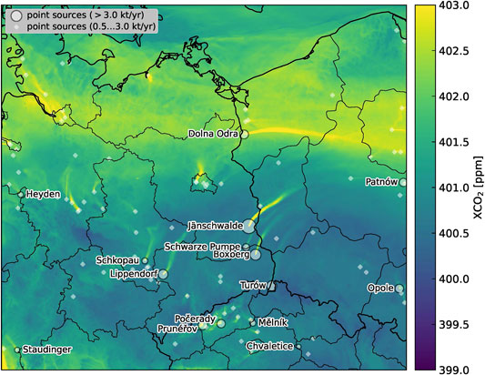
FIGURE 1. COSMO-GHG model domain with spatial distribution of the largest point sources (white dots). The image shows an example XCO2 model field on November 2, 2015.
Synthetic observations were then generated from the high resolution simulations for a hypothetical constellation of six CO2M satellites using orbit simulations and applying different levels of noise according to different precision requirements as specified by ESA. The satellites were assumed to fly in a sun-synchronous orbit with an overpass time of 11:30 local time. In each constellation, satellites were spaced with equal angular distance in a common orbit. As an example, Figure 2 shows a constellation of six satellites. Constellations of two or three satellites could then be composed, for example, of the satellites “a” and “d” or “a”, “c” and “e”, respectively.
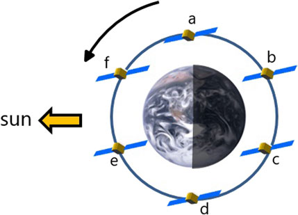
FIGURE 2. Sketch of a constellation of six CO2M satellites (a–f) equally spaced in a common sun-synchronous orbit.
To generate the synthetic observations of XCO2 and tropospheric columns of NO2, the simulated fields were sampled along the 250 km wide swath of the six orbits and mapped onto satellite pixels of the size of 2 km × 2 km. A low and high-noise instrument scenario was created for both the XCO2 and
2.2 CO2 and NOx Emissions of Point Sources
Plume detection and emission quantification was performed for the 15 largest point sources in the domain (all being power plants), which are labeled in Figure 1 by their names. Their annual mean CO2 and NOx emissions at satellite overpass time (10:30 UTC) as used in the simulations are listed in Table 1. The values are approximately 20% higher than true annual mean emissions due to the diurnal cycle of the emissions prescribed in the simulations and the CO2M overpass time. The three largest power plants have CO2 emissions comparable or larger than those of the city of Berlin with 20 Mt yr−1.
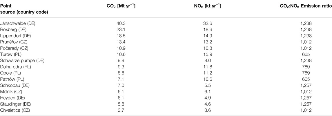
TABLE 1.
The CO2 and NOx emissions used in this study are based on the TNO/MACC-3 inventory for the year 2015. However, since 2017 a new EU regulation is in effect that requires a significant reduction of NOx emissions for large combustion plants (European Commission, 2017, Table 3). For lignite-fuelled power plants, the regulation requires new plants built after ratification of the regulation to reduce NOx concentrations in the flue gas to 50–85 mg m−3. Existing power plants need to reduce flue gas concentrations to <85–150 mg m−3 by 2021. NOX concentrations of up to 200 mg m−3 were allowed prior to the new regulation.
Based on reported NOx flue gas concentrations for German power plants (Tebert, 2017), we expect that for existing power plants NOx emissions will be reduced by 20–50% compared to the emissions assumed in our simulations. Power plants built after 2017 would have even lower emissions up to a third of the assumed levels. To study the influence of a future reduction of NOx emissions on our results, we scale anthropogenic NOx fields in the simulations with factors of 0.3, 0.5, and 0.8.
Since CO2 emissions are not affected by these regulations, CO2:NOX emission ratios will increase in the future. Table 1 shows that emission ratios (on a mass per mass basis) are considerably lower in the Czech Republic (CZ) and Poland (PL) than in Germany (DE), suggesting that stronger NOX reductions will be required in these countries to fulfill the new regulation. Supplementary Table S1 shows emission ratios for 2015 and 2017 based on self-reported emissions published in the E-PRTR database in 2019. For many power plants higher emission ratios are reported for 2017 compared to 2015 and also compared to the ratios used in our study, likely because operators already started strengthening emission reduction procedures. Note that emissions of point sources in the TNO/MACC-3 inventory can deviate somewhat from the E-PRTR database, because emissions from point sources were scaled in TNO/MACC-3 to resolve discrepancies between national totals and the totals of all individual point sources within a country (H. Denier van der Gon, personal communication).
2.3 Plume Detection Algorithm
A first version of our plume detection algorithm was presented in Kuhlmann et al. (2019a). The algorithm identifies coherent structures of satellite pixels of CO2 or NO2 that are significantly enhanced above background, and assigns these structures to a source. Emission plumes can either be detected from CO2 or from NO2 observations. With the first version of our algorithm we could demonstrate that CO2 emission plumes can be detected better from NO2 observations due to their higher signal-to-noise ratio and lower sensitivity to clouds (Kuhlmann et al., 2019a).
An important limitation of the first version was that the background within the plume was derived from a simulated background tracer. It thus relied on information that would not be available from real satellite observations. Furthermore, the algorithm required a large degree of fine-tuning and visual control. In order to overcome these limitations, an improved version was developed here, which does not depend on model simulated background fields anymore. Furthermore, the algorithm can now detect a predefined list of sources instead of a single source, and automatically recognizes overlapping plumes originating from multiple sources.
The improved algorithm consists of four steps described in the following. In the first step, pixels significantly enhanced above background are detected based on a statistical test applied to the following signal-to-noise ratio (SNR):
where
Instead of taking
In the first version of the algorithm, the background field was derived from a simulated background tracer. In the improved version, it is computed by applying a median filter to the satellite image. The filter computes the background as the local median in a 100 × 100 pixels window, assuming that the majority of pixels in the window consists of background pixels outside of the plume.
The random noise
The threshold
In the second step, the detected pixels are grouped into regions (plumes). A standard labeling algorithm is used for this purpose. Enhanced pixels are considered connected if they are horizontal, vertical or diagonal neighbors.
In the third step, a region of enhanced pixels is assigned to a point source, if the pixels overlap with a circle of radius 5 km surrounding the source. The improved version of the algorithm is now able to detect and flag plumes, that actually represent overlapping plumes originating from multiple sources. For this purpose we created a list of all point sources in the model domain that have NOx emissions larger than 3 kt yr−1 based on the TNO/MACC-3 inventory. Figure 1 shows a map of the XNO2 field simulated for November 3, 2015 and the location of the 15 largest sources.
In the fourth step, a centerline is fitted for each plume as a two-dimensional curve to the detected pixels. We include pixels outside of the plume within a distance of 5 km with low weight to make the fit more robust especially at the start and end of the plume. We also add the source location with high weight to force the centerline through that point. Finally, a polygon is drawn around the plume that follows the centerline and extends over the full width of the plume.
Figure 3 shows an example of the output of the algorithm. Longitude and latitude of the detected pixels are converted to a plume coordinate system consisting of arc length of the centerline from the source location and distance perpendicular to the centerline (see Kuhlmann et al., 2020a, for details). The width of the polygon corresponds to the maximum width of the detected plume rounded up to the next full 2 km. In along-plume direction, the polygon extends from the source to the end of the plume rounded up to the next full 5 km. The polygon is divided in 5 km wide sub-polygons in along-plume direction. In addition, a second polygon is drawn between 2 and 12 km upstream of the source that provides information about CO2 values upstream of the source. The different polygons and sub-polygons are required for the mass-balance method as described below.
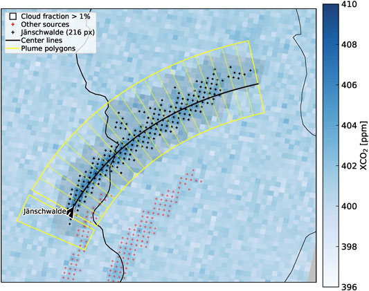
FIGURE 3. Sketch of detected CO2 plume with detected pixels, center line, and the polygon up- and downstream of the source.
2.4 Mass-Balance Approach
Emissions of a source can be estimated as the difference between the mass flux into and out of a volume containing the source. Here, fluxes out of the volume were computed as the fluxes through the sub-polygons determined by the plume detection algorithm downstream of the source. Under the assumption of steady-state conditions, this is equivalent to the emission, since the inflow upstream of the source is zero if we only consider enhancements above background. The only additional information that cannot be deduced from the satellite observations is an estimate of the wind speed inside the plume.
The fluxes are the product of line densities and wind speed. Line densities (units of kg m−1) are computed by integrating total column densities (units of kg m−2) perpendicular to the plume’s centerline. To obtain the column densities attributable to the source, the background field needs to be subtracted. The background was estimated from the pixels surrounding the plume assuming that it is a spatially smooth field. For this purpose, the detected pixels of the plume as well as other pixels marked as significantly enhanced above background by the plume detection algorithm were removed. The resulting gaps were then filled using normalized convolution with a Gaussian filter of width σ = 10 pixels. To have a consistent method for the estimation of CO2 and NOx emissions, we always compute the CO2 and NO2 background from the same detected pixels.
Note that the plume detection algorithm already required an estimation of the CO2 or NO2 background field. However, the background levels computed by that more simple algorithm were found to be generally overestimated (as compared to the true simulated background). Using that background would therefore result in an underestimation of the CO2 emissions.
After subtracting the background, line densities were computed by integrating the column densities in across-plume direction. To maximize the usage of information contained in the image, this was done for all sub-polygons every 5 km along the plume (Figure 3) by fitting a Gaussian curve
with total column density enhancement in the plume
To convert line densities into a flux, the effective transport wind speed u of the plume is required. This wind speed should correspond to the mean speed of horizontal transport of the tracer and therefore needs to account for different flow speeds at different altitudes. Since the vertical distribution of the mass of the emitted tracer cannot be deduced from the satellite observations and will usually not be known, simplified assumptions have to be made. Here, we assume that the distribution corresponds to the vertical emission profile for combustion in the energy sector (SNAP-1). This profile was used in the simulations for most power plants except for some of the largest ones (Boxberg, Jänschwalde, Lippendorf, Schwarze Pumpe, Turów, Patnów), for which plume rise was computed explicitly (Brunner et al., 2019). With this assumption, the wind speed was computed as the vertically averaged horizontal wind speed (from the COSMO-GHG model) at the source location and at the time of the overpass weighted by the SNAP-1 emission profile.
For
with
Equations 2, 3 were solved using the trust region reflective algorithm (Branch et al., 1999) implemented in the Python Scipy library (Version 1.4.1, Virtanen et al., 2020). The algorithm allows defining bounds for the fitting parameters, which was used to avoid negative line densities and emissions (see Supplementary Table S2 in the supplement).
Several checks have been implemented to avoid erroneous detection and correspondingly wrong emission estimates. The criteria have been chosen to be easily applicable to real observations and to avoid visual inspection of the results as much as possible. The checks are the following:
• Plumes are not used when they overlap more than one source.
• Plumes are not used when the direction of the center curve and the wind direction disagree by more than ± 45°.
• Plumes are not used when the “upstream polygon” contains more than five detected plume pixels. This criterion removes cases where the plume overlaps with an upstream source that is outside the swath or covered by clouds.
• Line densities are not computed for polygons that do not have valid satellite observations inside the detected plume every 5 km in across plume direction. The criterion removes misfits when observations near the plume center are missing.
• Line densities are not computed when the sub-polygon is not fully inside the swath.
• Line densities or fitted emissions are not used when the curve fit failed, because the number of observations/fluxes was too small or their uncertainties were too large.
2.5 Uncertainties
Uncertainties of the mass-balance approach are caused by instrument noise, uncertainties in the effective transport wind speed, uncertainties in estimating the background, and a general “methodological uncertainty” such as the assumption of steady-state conditions.
Since the number of successful estimates is relatively small and varies strongly between the sources, we tested and compared several different ways of estimating the systematic and random uncertainties. The first approach is based on comparing the estimated emissions to the true emissions, which are known in our synthetic model framework but would not be known in reality. Differences between estimated and true emissions were used to compute a median bias (MB) and standard deviation (SD). Relative values were computed by dividing by the mean emissions at satellite overpass time (10:30 UTC). Since the differences are not necessarily normally distributed, we computed the 16–84th percentile range (PR) and divided this range by two to be comparable with the standard deviation.
In a second approach, which is also applicable to real observations without knowledge of the true emissions, the uncertainty is computed by error propagation from the uncertainties in line density
Here,
Additional uncertainties due methodological and background errors are difficult to quantify. In order to provide a realistic estimate of the overall uncertainty, we add to the emission uncertainty described in Eq. 4 a constant factor m proportional to the emission strength and add an offset b, so that the overall uncertainty is consistent with the PRs estimated by the first approach. PRs are used because SDs overestimate the variance of the estimates due to outliers. The uncertainty is then given by
where Q is the
Estimating the uncertainty of the
2.6 Annual Emissions and Emission Ratios
The accuracy of an annual mean estimate derived from individual overpasses on a small number of days depends critically on how well the temporal variability of emissions is captured. In this study, the COSMO-GHG simulations used hourly emission fields as input, which were derived from annual emissions using fixed diurnal, weekly and seasonal time profiles (see Supplementary Figure S2) for the different source categories of the Selected Nomenclature for Air Pollution (SNAP) (Pouliot et al., 2012; Jähn et al., 2020). At satellite overpass, both
Annual emissions were obtained by fitting a low order C-spline to the individual estimates collected by all satellites present in a constellation of a given size. We used periodic boundary conditions to smoothly connect the end and the beginning of the year. The fitted curve is then integrated to obtain annual emissions. Their uncertainties are estimated by error propagation from the random uncertainties of the individual estimates. The low-order spline accounts for a seasonal cycle varying slowly with time but does not account for more rapid day-to-day variability.
Since CO2M is in a sun-synchronous orbit with fixed overpass time, individual estimates are only representative of emissions a few hours before the satellite overpass but not for the daily mean (Broquet et al., 2018). It is therefore necessary to apply a correction factor to obtain true annual mean emissions, which introduces an additional source of uncertainty. We assume here that a mean diurnal cycle can be obtained from electricity demand statistics or other observations (e.g., ground-based monitoring networks or geostationary satellites), while deviations from such a mean behavior need to be accounted for in the uncertainty budget.
Hill and Nassar (2019) analyzed the hour-to-hour and day-to-day variability of emissions for the 50 largest power plants in the United States. They found that after subtracting a mean seasonal and diurnal cycle, the remaining hour-to-hour
where
Note that we do not apply any sampling bias correction factor for the diurnal cycle but compare with the annual mean emissions at satellite overpass. Since our results (e.g., detection threshold and uncertainties) depend on the emission strength at overpass, this makes it easier to generalize our results in case diurnal cycles are different.
2.7 Quantitative Usage of NO2 Observations
Since
The emission ratio is used to convert the estimated annual
3 Results
3.1 Example of Individual CO2 and NOx Emission Estimates
Figure 4 shows examples of detected plumes from
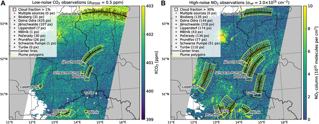
FIGURE 4. Comparing plume detection using (A) CO2 observations with low noise (
Figure 5 shows an example of the application of the mass-balance approach for the coal-fired power plant near Mělník (CZ). The true
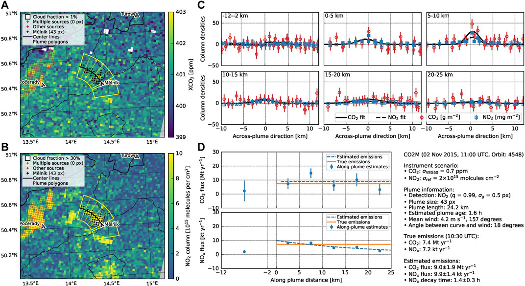
FIGURE 5. Exemplary application of the mass balance approach for the point source near Mělník (CZ). (A) CO2 and (B) NO2 satellite image with detected plumes and polygons for computing line densities. (C) Across plume CO2 and NO2 values for the six polygons and fitted Gaussian curves. (D) CO2 and NOx fluxes along the centerline and estimated CO2 and NOx emissions.
The centerline was fitted to the 43 satellite pixels of the detected
The plume length of 24 km allows drawing five polygons for subsequent mass balance analysis. Figure 5C shows
3.2 Number of Successful CO2 and NOx Emission Estimates
The number of successful
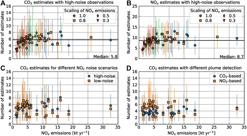
FIGURE 6. Number of successful (A)
Figure 6A shows the number of successful
For these weak
The number of successful
The number of successful estimates of
3.3 Uncertainty of Individual Emission Estimates
The total estimated random uncertainties were computed with Eq. 5. The median uncertainties obtained from the mass-balance algorithm
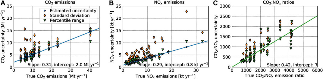
FIGURE 7. Random uncertainty of estimated (A)
For weak sources (<10 Mt yr–1), the total
For
Figure 7C shows SDs and PRs of the individual
The
3.4 Distribution of Emission Estimates Over the Year
How well annual mean emissions can be quantified depends on the number of individual estimates available during a year and on how well they capture temporal variability including the seasonal cycle of emissions. As an example, Figure 8 shows the time series of estimates of
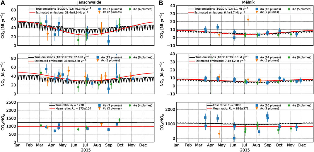
FIGURE 8. Time series of estimated
At Jänschwalde, 13 successful
As mentioned above, the annual mean emissions were computed by integrating the C-spline fitted to the individual estimates. At Mělník, the shape of the seasonal cycle is fitted well. The annual
3.5 Annual Emissions
Figure 9 compares annual mean estimates obtained for all 15 power plants with true annual emissions at satellite overpass (10:30 UTC) for high-noise
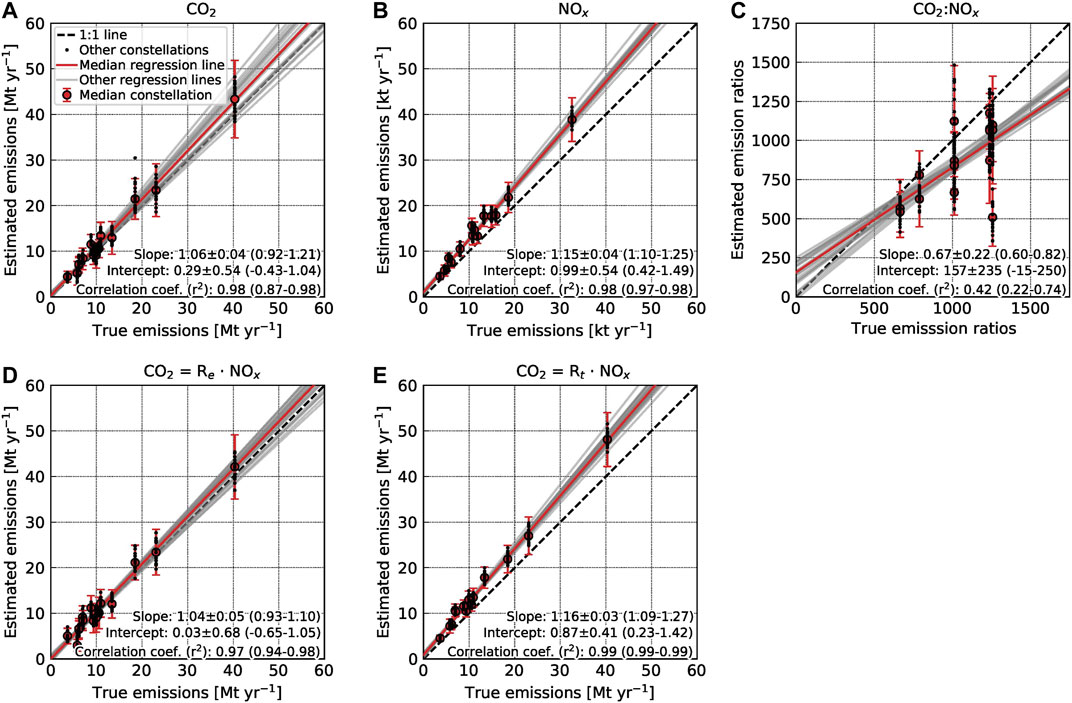
FIGURE 9. Annual estimates of (A)
The
Figure 9C compares the estimated annual mean ratios with the true emission ratios. The correlation between estimated and true emission ratios is quite low with
Figures 9D,E compare
Figure 10 shows the estimated uncertainty of annual
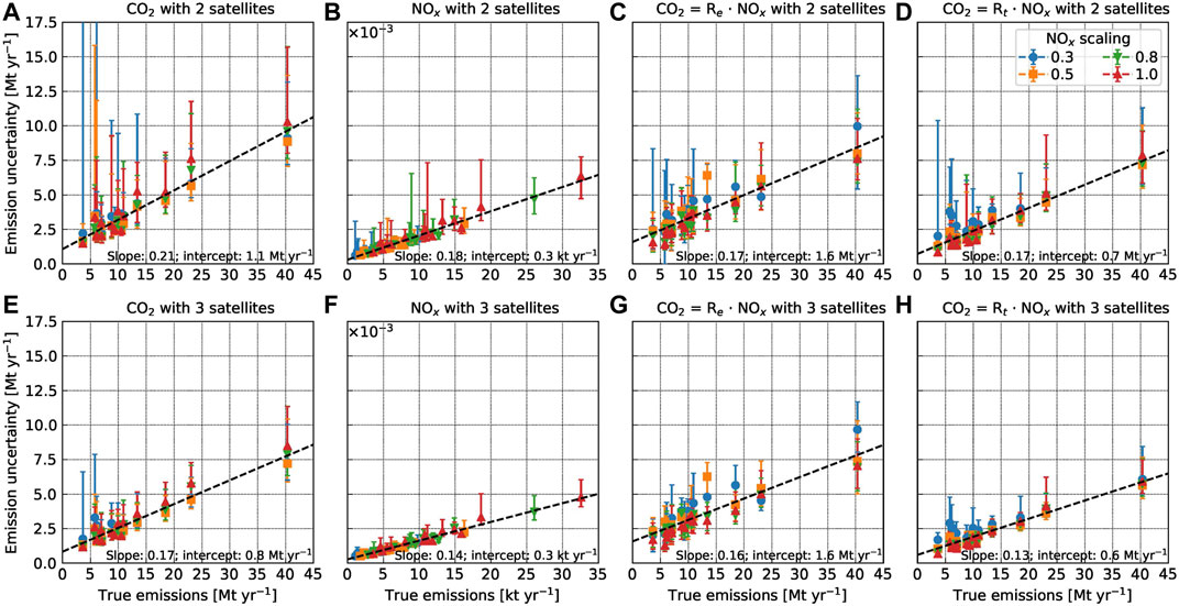
FIGURE 10. Estimated uncertainty of annual mean of emissions of (A)
Uncertainties range from 23–119% and 18–65% for CO2 emission estimates for two and three satellites, respectively, considering the future reduction of NOx emissions. For NOx emissions, uncertainties range from 16–73% and 13–52% for two and three satellites, respectively. In general, the uncertainty is proportional to the source strength Q and can be described by a regression line with slope m and intercept b. For
When
The median uncertainties are only slightly smaller for three satellites than for two, but the range between individual constellations is much smaller. A constellation of three satellites is thus less likely to produce highly uncertain results due to insufficient coverage than a constellation of two.
Figure 11A shows the number of annual
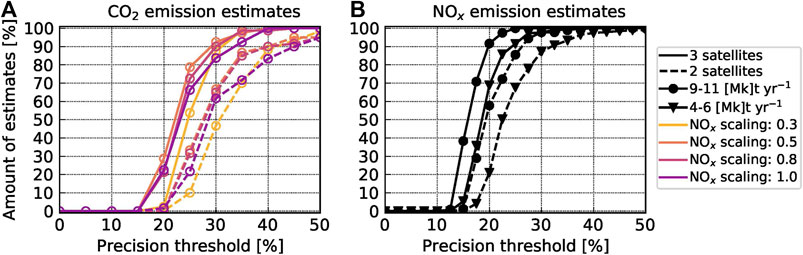
FIGURE 11. Number of successful (A)
In terms of annual
3.6 Global Application of the Mass-Balance Approach
The mass-balance approach can be applied globally, because it does not require any additional expensive atmospheric transport simulations, but solely relies on wind information that is available from global analysis and reanalysis products. A database of points sources is available through the global map of emissions clumps (Wang et al., 2019), which lists about 900 point sources with
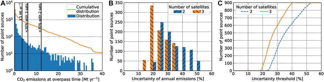
FIGURE 12. (A) Distribution of point sources based on
To upscale our results, we use the regression lines found for the uncertainties of annual emissions (Figures 10A,E) to calculate uncertainties of all point sources. We expect that our results are sufficiently representative for the sources in the database, because about 90% of them are located in the mid-latitudes (23.4°–66.5°) like our study area (50°N—55°N) and thus have a similar number of satellite overpasses ranging from 1.1 to 2.7 per 11 days repeat cycle compared to 1.7 in our study area.
Figure 12B shows the uncertainties of annual emissions computed for the 900 point sources for a constellation of two and three satellites showing that adding a third satellite reduces uncertainties from 35 to 28% on average. As a result, two satellites would be able to quantify annual emissions with an uncertainty <30% for only 300 point sources, while three satellites could quantify emissions for 600 point sources (Figure 12C). The 300 and 600 sources account for total emissions of 6,000 Mt yr–1 and 8,700 Mt yr–1, which are about 16 and 24% of global anthropogenic emissions.
Therefore, adding a third CO2M satellite has the potential to double the number of quantifiable point sources. Since our analysis used the regression lines in Figure 10, the numbers are likely overestimated, because some point sources are insufficiently covered by the satellites (Figure 11). However, this would especially affect a constellation of two satellites making it likely that we still underestimate the benefit of a third satellite here.
4 Discussion
In this study, we used synthetic CO2M satellite observations to investigate the potential of a constellation of
We have developed an advanced data-driven method to quantify point source emissions in a semi-automated way. The method identifies the location of power plant plumes using a plume detection algorithm and quantifies both
Individual
The uncertainties in our emission estimates are dominated by uncertainties in the
For a constellation of two satellites, annual CO2 and NOx emissions were estimated with an uncertainty of 23–119% and 16–73%, respectively. Adding a third CO2M satellite reduced uncertainties to 18–65% for CO2 and 13–52% for NOx emission estimates. The uncertainty includes an estimate of the uncertainty in the temporal variability of emissions that accounts for about 50% to the total uncertainty. Since annual
In our simulations, we assumed a constant
Our study shows that CO2M will likely be able to quantify
The mass-balance approach applied in this study has the advantage that it can be applied easily without expensive atmospheric transport simulations. However, the approach suffers from relatively high uncertainties of individual estimates for complex plumes and from uncertainties associated with the sparse temporal sampling of the varying emissions. Estimates could be significantly improved with additional information, for example, from atmospheric transport simulations, energy demand statistics and additional observations (e.g., ground-based networks and geostationary NO2 satellites). Such information will become available, for example, through the future Copernicus
Data Availability Statement
The original contributions presented in the study are included in the article/Supplementary Material, further inquiries can be directed to the corresponding author. The Python code used for detecting the plumes and quantifying the emissions is publicly available at: https://gitlab.com/empa503/remote-sensing/ddeq.
Author Contributions
GK developed, implemented, applied and evaluated the methods for estimating CO2 emissions, and wrote the manuscript with input from all co-authors. DB supervised and led the SMARTCARB-2 project. SH was member of the SMARTCARB-2 project team and contributed critical input to the manuscript. YM accompanied the study as ESA project officer and provided critical inputs and reviews during all phases of the project.
Funding
This study was conducted in the context of the project SMARTCARB funded by the European Space Agency (ESA) under contract no. 4000119599/16/NL/FF/mg and supported by the EU Horizon-2020 project CHE under grant no. 776186. The views expressed here can in no way be taken to reflect the official opinion of ESA. COSMO-GHG calculations were carried out at the Swiss National Supercomputing Center (CSCS) under project ID s862.
Conflict of Interest
The authors declare that the research was conducted in the absence of any commercial or financial relationships that could be construed as a potential conflict of interest.
Supplementary Material
The Supplementary Material for this article can be found online at: https://www.frontiersin.org/articles/10.3389/frsen.2021.689838/full#supplementary-material
References
Beirle, S., Boersma, K. F., Platt, U., Lawrence, M. G., and Wagner, T. (2011). Megacity Emissions and Lifetimes of Nitrogen Oxides Probed from Space. Science 333, 1737–1739. doi:10.1126/science.1207824
Bovensmann, H., Buchwitz, M., Burrows, J. P., Reuter, M., Krings, T., Gerilowski, K., et al. (2010). A Remote Sensing Technique for Global Monitoring of Power Plant CO2 Emissions from Space and Related Applications. Atmos. Meas. Tech. 3, 781–811. doi:10.5194/amt-3-781-2010
Branch, M. A., Coleman, T. F., and Li, Y. (1999). A Subspace, interior, and Conjugate Gradient Method for Large-Scale Bound-Constrained Minimization Problems. SIAM J. Sci. Comput. 21, 1–23. doi:10.1137/S1064827595289108
Broquet, G., Bréon, F.-M., Renault, E., Buchwitz, M., Reuter, M., Bovensmann, H., et al. (2018). The Potential of Satellite Spectro-Imagery for Monitoring CO2 Emissions from Large Cities. Atmos. Meas. Tech. 11, 681–708. doi:10.5194/amt-11-681-2018
Brunner, D., Kuhlmann, G., Marshall, J., Clément, V., Fuhrer, O., Broquet, G., et al. (2019). Accounting for the Vertical Distribution of Emissions in Atmospheric CO2 Simulations. Atmos. Chem. Phys. 19, 4541–4559. doi:10.5194/acp-19-4541-2019
Buchwitz, M., Reuter, M., Bovensmann, H., Pillai, D., Heymann, J., Schneising, O., et al. (2013). Carbon Monitoring Satellite (CarbonSat): Assessment of Atmospheric CO2 and CH4 Retrieval Errors by Error Parameterization. Atmos. Meas. Tech. 6, 3477–3500. doi:10.5194/amt-6-3477-2013
Ciais, P., Crisp, D., Gon, H. v. d., Engelen, R., Heimann, M., Janssens-Maenhout, G., et al. (2015). Towards a European Operational Observing System To Monitor Fossil CO2 Emissions - Final Report From the Expert Group. European Commission, Copernicus Climate Change Service. Report
Düring, I., Bächlin, W., Ketzel, M., Baum, A., Friedrich, U., and Wurzler, S. (2011). A New Simplified NO/NO2 Conversion Model under Consideration of Direct NO2-Emissions. metz 20, 67–73. doi:10.1127/0941-2948/2011/0491
ESA Earth and Mission Science Division, (2020). Tech. rep. Version 3.0. Copernicus CO2 Monitoring Mission Requirements Document (MRD), Available at: https://esamultimedia.esa.int/docs/EarthObservation/CO2M_MRD_v3.0_20201001_Issued.pdf. (access:1 October 2020)
European Commission (2017). Commission Implementing Decision (EU) 2017/1442 of 31 July 2017 Establishing Best Available Techniques (BAT) Conclusions, under Directive 2010/75/eu of the European Parliament and of the Council, for Large Combustion Plants (Notified under Document C(2017) 5225) (Text with EEA relevance.). Available at: https://eur-lex.europa.eu/eli/dec_impl/2017/1442/oj (Accessed July 31, 2017).
Fioletov, V. E., McLinden, C. A., Krotkov, N., and Li, C. (2015). Lifetimes and Emissions of SO2 from point Sources Estimated from OMI. Geophys. Res. Lett. 42, 1969–1976. doi:10.1002/2015GL063148
Hill, T., and Nassar, R. (2019). Pixel Size and Revisit Rate Requirements for Monitoring Power Plant CO2 Emissions from Space. Remote Sensing 11, 1608. doi:10.3390/rs11131608
Houweling, S., Landgraf, J., van Heck, H., Vlemmix, T., and Tao, W. (2019). AEROCARB – Study on Use of Aerosol Information for Estimating Fossil CO2 Emissions - Final Report: Synthesis and Recommendation of ESA Study RFP/3-14860/17./NL/FF/gp. Version 2.0 Tech. rep
Jähn, M., Kuhlmann, G., Mu, Q., Haussaire, J.-M., Ochsner, D., Osterried, K., et al. (2020). An Online Emission Module for Atmospheric Chemistry Transport Models: Implementation in COSMO-GHG v5.6a and COSMO-ART v5.1-3.1. Geosci. Model. Dev. 13, 2379–2392. doi:10.5194/gmd-13-2379-2020
Janssens-Maenhout, G., Pinty, B., Dowell, M., Zunker, H., Andersson, E., Balsamo, G., et al. (2020). Toward an Operational Anthropogenic CO2 Emissions Monitoring and Verification Support Capacity. Bull. Am. Meteorol. Soc. 101, E1439–E1451. doi:10.1175/BAMS-D-19-0017.1
Kuhlmann, G., Broquet, G., Marshall, J., Clément, V., Löscher, A., Meijer, Y., et al. (2019a). Detectability of CO2 Emission Plumes of Cities and Power Plants with the Copernicus Anthropogenic CO2 Monitoring (CO2M) mission. Atmos. Meas. Tech. 12, 6695–6719. doi:10.5194/amt-12-6695-2019
Kuhlmann, G., Brunner, D., Broquet, G., and Meijer, Y. (2020a). Quantifying CO2 Emissions of a City with the Copernicus Anthropogenic CO2 Monitoring Satellite mission. Atmos. Meas. Tech. 13, 6733–6754. doi:10.5194/amt-13-6733-2020
Kuhlmann, G., Clément, V., Marschall, J., Fuhrer, O., Broquet, G., Schnadt-Poberaj, C., et al. (2019b). SMARTCARB - Use of Satellite Measurements of Auxiliary Reactive Trace Gases for Fossil Fuel Carbon Dioxide Emission Estimation, Final Report of ESA Study Contract n°4000119599/16/NL/FF/mg. Tech. rep., Empa, Swiss Federal Laboratories for Materials Science and Technology. Switzerland: Dübendorf. doi:10.5281/zenodo.4034266
Kuhlmann, G., Clément, V., Marshall, J., Fuhrer, O., Broquet, G., Schnadt-Poberaj, C., et al. (2020b). Synthetic XCO2, CO and NO2 Observations for the CO2M and Sentinel-5 Satellites. doi:10.5281/zenodo.4048228
Kuhlmann, G., Henne, S., Löscher, A., Meijer, Y., and Brunner, D. (2021). SMARTCARB 2 – Use Of Satellite Measurements of Auxiliary Reactive Trace Gases for Fossil Fuel Carbon Dioxide Emission Estimation (Phase 2), Final Report Of ESA Study Contract n4000119599/16/NL/FF/mg. Tech. rep., Empa, Swiss Federal Laboratories for Materials Science and Technology. Switzerland: Dübendorf. doi:10.5281/zenodo.4674167
Lespinas, F., Wang, Y., Broquet, G., Bréon, F.-M., Buchwitz, M., Reuter, M., et al. (2020). The Potential of a Constellation of Low Earth Orbit Satellite Imagers to Monitor Worldwide Fossil Fuel CO2 Emissions from Large Cities and point Sources. Carbon Balance Manage 15, 1–12. doi:10.1186/s13021-020-00153-4
Lorente, A., Boersma, K. F., Eskes, H. J., Veefkind, J. P., Van Geffen, J. H. G. M., de Zeeuw, M. B., et al. (2019). Quantification of Nitrogen Oxides Emissions from Build-Up of Pollution over Paris with TROPOMI. Sci. Rep. 9, 1–10. doi:10.1038/s41598-019-56428-5
Martin, A., Weissmann, M., Reitebuch, O., Rennie, M., Geiß, A., and Cress, A. (2021). Validation of Aeolus Winds Using Radiosonde Observations and Numerical Weather Prediction Model Equivalents. Atmos. Meas. Tech. 14, 2167–2183. doi:10.5194/amt-14-2167-2021
Nassar, R., Hill, T. G., McLinden, C. A., Wunch, D., Jones, D. B. A., and Crisp, D. (2017). Quantifying CO2 Emissions from Individual Power Plants from Space. Geophys. Res. Lett. 44 (10), 917–933. doi:10.1002/2017GL074702
Nassar, R., Napier-Linton, L., Gurney, K. R., Andres, R. J., Oda, T., Vogel, F. R., et al. (2013). Improving the Temporal and Spatial Distribution of CO2 Emissions from Global Fossil Fuel Emission Data Sets. J. Geophys. Res. Atmos. 118, 917–933. doi:10.1029/2012JD018196
Pillai, D., Buchwitz, M., Gerbig, C., Koch, T., Reuter, M., Bovensmann, H., et al. (2016). Tracking City CO2 Emissions from Space Using a High-Resolution Inverse Modelling Approach: a Case Study for Berlin, Germany. Atmos. Chem. Phys. 16, 9591–9610. doi:10.5194/acp-16-9591-2016
Pinty, B., Janssens-Maenhout, G., Dowell, M., Zunker, H., Brunhe, T., Ciais, P., et al. (2018). An Operational Anthropogenic CO2 Emissions Monitoring & Verification Support Capacity - Baseline Requirements, Model Components And Functional Architecture. Report. doi:10.2760/39384
Pouliot, G., Pierce, T., Denier van der Gon, H., Schaap, M., Moran, M., and Nopmongcol, U. (2012). Comparing Emission Inventories and Model-Ready Emission Datasets between Europe and North America for the AQMEII Project. Atmos. Environ., 53, 4–14. doi:10.1016/j.atmosenv.2011.12.041
Reum, F., and Houweling, S. (2020). Impact of Urban Aerosols on Satellite-Retrieved CO2, CHE Project, Deliverable 2.7 Tech. Rep. Available at:https://www.che-project.eu/sites/default/files/2020-12/CHE-D2-7-V1-0.pdf (access: May 20, 2021).
Reuter, M., Buchwitz, M., Hilboll, A., Richter, A., Schneising, O., Hilker, M., et al. (2014). Decreasing Emissions of NOx Relative to CO2 in East Asia Inferred from Satellite Observations. Nat. Geosci 7, 792–795. doi:10.1038/ngeo2257
Reuter, M., Buchwitz, M., Schneising, O., Krautwurst, S., O'Dell, C. W., Richter, A., et al. (2019). Towards Monitoring Localized CO2 Emissions from Space: Co-located Regional CO2 and NO2 Enhancements Observed by the OCO-2 and S5P Satellites. Atmos. Chem. Phys. 19, 9371–9383. doi:10.5194/acp-19-9371-2019
Rockström, J., Gaffney, O., Rogelj, J., Meinshausen, M., Nakicenovic, N., and Schellnhuber, H. J. (2017). A Roadmap for Rapid Decarbonization. Science 355, 1269–1271. doi:10.1126/science.aah3443
Rusli, S. P., Hasekamp, O., aan de Brugh, J., Fu, G., Meijer, Y., and Landgraf, J. (2021). Anthropogenic CO2 Monitoring Satellite mission: the Need for Multi-Angle Polarimetric Observations. Atmos. Meas. Tech. 14, 1167–1190. doi:10.5194/amt-14-1167-2021
Sierk, B., Bézy, J.-L., Löscher, A., and Meijer, Y. (2019). The European CO2 Monitoring Mission: Observing Anthropogenic Greenhouse Gas Emissions from Space 11180. Proceedings, International Conference on Space Optics — ICSO 2018. 12 July 2019. Chania, Greece. 111800M. doi:10.1117/12.2535941
Super, I., Dellaert, S. N. C., Visschedijk, A. J. H., and Denier van der Gon, H. A. C. (2020). Uncertainty Analysis of a European High-Resolution Emission Inventory of CO2 and CO to Support Inverse Modelling and Network Design. Atmos. Chem. Phys. 20, 1795–1816. doi:10.5194/acp-20-1795-2020
Tebert, C. (2017). Stickstoffoxid-Emissionen aus Kohlekraftwerken: Minderungspotenzial auf Basis von Messdaten der Jahre 2016 und 2017,Tech. rep. Auftraggeber: Bund für Umwelt und Naturschutz Deutschland e.V. (BUND) und Klima-Allianz Deutschland. Available at: https://www.bund.net/fileadmin/user_upload_bund/publikationen/kohle/kohle_stickoxid_emissionen_gutachten.pdf (access:September 2, 2020).
UNFCCC (2015). Paris Agreement, FCCC/CP/2015/L.9/Rev1. Available at: http://unfccc.int/resource/docs/2015/cop21/eng/l09r01.pdf.
Varon, D. J., Jacob, D. J., McKeever, J., Jervis, D., Durak, B. O. A., Xia, Y., et al. (2018). Quantifying Methane point Sources from fine-scale Satellite Observations of Atmospheric Methane Plumes. Atmos. Meas. Tech. 11, 5673–5686. doi:10.5194/amt-11-5673-2018
Virtanen, P., Gommers, R., Gommers, R., Oliphant, T. E., Haberland, M., Reddy, T., et al. (2020). SciPy 1.0: Fundamental Algorithms for Scientific Computing in Python. Nat. Methods 17, 261–272. doi:10.1038/s41592-019-0686-2
Wang, Y., Broquet, G., Bréon, F.-M., Lespinas, F., Buchwitz, M., Reuter, M., et al. (2020). PMIF v1.0: Assessing the Potential of Satellite Observations to Constrain CO2 Emissions from Large Cities and point Sources over the globe Using Synthetic Data. Geosci. Model. Dev. 13, 5813–5831. doi:10.5194/gmd-13-5813-2020
Wang, Y., Ciais, P., Broquet, G., Bréon, F.-M., Oda, T., Lespinas, F., et al. (2019). A Global Map of Emission Clumps for Future Monitoring of Fossil Fuel CO2 Emissions from Space. Earth Syst. Sci. Data 11, 687–703. doi:10.5194/essd-11-687-2019
Wolff, S., Ehret, G., Kiemle, C., Amediek, A., Quatrevalet, M., Wirth, M., et al. (2020). Determination of the Emission Rates of CO2 Point Sources with Airborne Lidar. Atmos. Meas. Tech. Discuss. 2020, 1–28. doi:10.5194/amt-2020-390
Wu, D., Lin, J. C., Oda, T., and Kort, E. A. (2020). Space-based Quantification of Per Capita CO2 Emissions from Cities. Environ. Res. Lett. 15, 035004. doi:10.1088/1748-9326/ab68eb
Keywords: CO2M, CO2, NO2, emission quantification, mass-balance approach, plume detection, coal power plants, imaging remote sensing
Citation: Kuhlmann G, Henne S, Meijer Y and Brunner D (2021) Quantifying CO2 Emissions of Power Plants With CO2 and NO2 Imaging Satellites. Front. Remote Sens. 2:689838. doi: 10.3389/frsen.2021.689838
Received: 01 April 2021; Accepted: 17 June 2021;
Published: 06 July 2021.
Edited by:
Jing Li, Peking University, ChinaReviewed by:
Xin Ma, Wuhan University, ChinaHusi Letu, Institute of Remote Sensing and Digital Earth (CAS), China
Copyright © 2021 Kuhlmann, Henne, Meijer and Brunner. This is an open-access article distributed under the terms of the Creative Commons Attribution License (CC BY). The use, distribution or reproduction in other forums is permitted, provided the original author(s) and the copyright owner(s) are credited and that the original publication in this journal is cited, in accordance with accepted academic practice. No use, distribution or reproduction is permitted which does not comply with these terms.
*Correspondence: Gerrit Kuhlmann, gerrit.kuhlmann@empa.ch