Abstract
In electrophysiology, many methods have been proposed for the analysis of action potential firing frequencies. The aim of this study was to present an algorithm developed for a continuous wavelet transform that enables the filtering out of frequencies contributing to the shapes of action potentials (spikes), whilst retaining the frequencies that encode the periodicity of spike trains. The continuous wavelet transform allows us to decompose a signal into its constituent frequencies. A signal with a single event, such as a spike, is composed of frequencies that characterize the shape of the spike. A signal with two spikes will also be composed of frequencies characterizing the shape of the action potential, but in addition will include a substantial portion of its power at the frequency corresponding to the time-difference between the two spikes. This is achieved by clipping peaks from the wavelet amplitudes that are narrower than a given minimum number of phase cycles. We present some application examples in both synthetic signals and electrophysiological recordings. This new approach can provide a major new analytical tool for analysis of electrophysiological signals.
1. Introduction
In electrophysiology, non-stationary quasiperiodic time series signals are common. The continuous wavelet transform (Mallat, 2008) is a useful tool for analysing such signals. It decomposes a time domain signal x(t) into the time-scale domain w(t, s), by cross-correlating x(t) with a wavelet function ψs(t) that contains an intrinsic frequency fs inversely proportional to scale s and localized about time t = 0. Intuitively, w(t, s) is a measure of the strength of oscillation of x(t) at a frequency fs within a neighborhood at time t of duration proportional to s.
The wavelet transform is ideally suited to measuring the time-varying frequencies of smoothly oscillating signals. However, in many cases, signals could be described as more “spiky” than “smooth.” A spiky signal is characterized by short-duration changes in amplitude separated by much longer quiescent periods, where each short-duration change is considered an event of interest and referred to as a “spike.” For such signals, even though the wavelet transform does capture the frequency at which the spikes occur, it also produces harmonic artifacts that capture the higher frequency changes characterizing the shape of each individual spike.
The conventional approach for measuring the frequency of spiky events is to identify the events via peak-detection (e.g., Nenadic and Burdick, 2005) and report the intervals between adjacent-in-time events. The main advantage of such an approach is that the precise locations-in-time of each event are found, and so the precise intervals between events can be obtained. In some application domains, such as spike sorting (Lewicki, 1998), event times as well as the event shapes need to be identified so that the signal can be decomposed into its additive component signals based on the shapes of events, and then the event frequencies calculated for each signal separately. Precise event times also allow for the inference of parameters of non-periodic activity, for example, the instantaneous rate of a Poisson point process (Adams et al., 2009). In such cases, the algorithm presented in this paper would be of limited use.
The algorithm presented here (in Algorithm 1), which we call “mesaclip,” does not identify individual events. Rather it clips amplitudes from the time-scale representation of a signal that span a period of time too short to contribute to multiple events. This is done by removing amplitudes from the result of a wavelet transform that are shorter than k cycles, where k is the algorithm's only parameter and k = 2 is an excellent default.
It should be noted that the purpose is not to remove spike data from the original time-domain signal, such as described in Ehrentreich and Sümmchen (2001) or Veneri et al. (2011). Retaining the spikes is essential to recovering the frequency of those events. An input spike event will have a transient “peaked” response at higher frequencies, and it is this response that is clipped, while the event's contribution to lower frequencies is retained, exposing the frequency of a train of such events.
A motivation for using the wavelet transform in conjunction with mesaclip, over peak detection, is the ability to reveal multiple simultaneous frequencies in a signal, such as the frequency of recurring bouts of events. Also, the phase of the signal at each frequency is retained, allowing for the phase-difference to be calculated against a second signal via the cross wavelet transform, a technique useful for computing interactions between two or more signals (Torrence and Webster, 1999; Bloomfield et al., 2004; Grinsted et al., 2004).
A recent approach, called de-shape, for removing the influence of the wave-shape from the time-frequency response is presented in Lin et al. (2018). It appears to have similar qualitative results to the algorithm presented in this paper. There, the short-time Fourier transform (STFT) is multiplied by the inverse short-time cepstral transform (iSTCT). The STFT contains the harmonic series, that is, integer multiples of the fundamental frequency, and the iSTCT contains a sub-harmonic series, which are integer divisions of the fundamental frequency. Multiplying the two removes the harmonics and retains the fundamental frequency.
This paper is organized as follows: section 2 gives a brief overview of the wavelet transform, section 3 describes the mesaclip algorithm that is the main contribution of this paper, section 4 presents results on real and synthetic signals, section 5 is a discussion of the results, limitations, and advantages, and section 6 concludes the paper.
2. Wavelet Transform
The wavelet transform converts a signal from the time-domain to the time-frequency domain, such that for each point in time there is a decomposition of the signal around that point in time into its constituent frequencies. More precisely, the transform converts to a time-scale domain, but appropriate mapping from scale to frequency can be chosen.
For computing the wavelet transform on an input signal x(t) ∈ ℝ, we choose a wavelet basis function ψ(t) ∈ ℂ and set of positive time scales S = {s1, …sL}. An admissible wavelet function is one which has zero mean and its Fourier transform is continuously differentiable (Farge, 1992), with an extra desirable property that it be localized in both time and frequency. For each scale, a wavelet is constructed by effectively stretching in time the wavelet basis function by that scale, while normalizing to unit energy (1).
To compute the transform, for each scale s ∈ S, we compute the cross-correlation of the signal with the wavelet (2). A finite set of scales is explicitly chosen here, since the algorithm presented in this paper operates on each scale independently, and to formalize this we've moved the scale argument into a subscript w(t, s) → ws(t). The resulting output is a time-scale representation of the signal, which can be mapped to a time-frequency representation by the reciprocal function f = c/s, for frequency f, scale s, and a ψ-dependent constant factor c. See Torrence and Compo (1998) or Mallat (2008) for an introduction to wavelet analysis.
Another way to map from scales to frequencies is via synchrosqueezing (Daubechies et al., 2011). Synchrosqueezing calculates the frequency not as a function of the scale but by redistributing the wavelet amplitudes based on the time-derivative of the phase (i.e., instantaneous frequency). This approach is included in the examples presented in this paper, although it is applied as a post-process to the mesaclip algorithm, that is, the redistribution of amplitudes occurs after they have been clipped.
3. MesaClip
The result of the wavelet transform, for a scale s ∈ S, can be written in polar-form as w(t) = r(t)eiϕ(t) for some time-varying amplitude r ∈ ℝ≥0 and phase ϕ ∈ ℝ (omitting explicit scale identification for brevity). An unwrapped phase ϕ is assumed, and that ϕ is non-decreasing . If the phase is not non-decreasing, then we set negative instantaneous frequencies to 0, thereby enforcing monotonicity.
A difference in phase from time t1 to time t2 of ϕ(t2)−ϕ(t1) = 2πk means there are k cycles over that time interval in the signal at the given scale s. A substantially high peak in r over this time-range suggests a substantially strong oscillation. If the width of such a peak is localized over a short phase-range, ϕ(t2)−ϕ(t1) <2πk, then the peak spans fewer than k cycles. If we clip the amplitude of all peaks that are narrower-in-phase than some given constant 2πk, down to an amplitude such that the tops of resulting plateaus are of width 2πk, then we will have effectively removed amplitudes contributing to oscillations shorter than k cycles.
To illustrate the idea of clipping formally, consider a function g(φ) = r(ϕ−1(φ)) that maps from phases to amplitudes1. We can wrap additional scaffolding around g with
which, for a given phase φ, finds the largest h such that there exists at least one non-empty phase interval [a, b] containing φ and where the amplitude at all elements of [a, b] is no less than h. Although (3) appears redundant, it allows us to now append the extra condition b−a≥κ, which specifies a minimum width κ for each interval, resulting in the function
For κ = 2πk, the function g2πk(φ) corresponds to one where the tops of narrow high peaks have been clipped away leaving lower plateaus of width no less than k cycles. Note, it is the peaks in the wavelet amplitudes that are clipped, not the spikes in the original time-domain signal.
A critical component of the algorithm is an appropriate choice of wavelet function. We use the Morse wavelet, which generalizes many conventional wavelet functions (Lilly and Olhede, 2012), and remains analytic even for highly time-localized instances. It admits two parameters, β and γ. We use a value of γ = 3 as it results in wavelets that are symmetric in frequency space and has a small Heisenberg area (Lilly and Olhede, 2009). We choose the value β = β* heuristically, where the value β* = 1.58174 minimizes (practically zeroes) the amplitude of the first harmonic of the wavelet transform of a Dirac comb, halfway between two successive Dirac delta functions. Since the discrete-time Fourier transform of a Dirac delta function is 1, then β* can be calculated (5) by numerically minimizing, at the middle time sample n = N/2, the absolute value of the inverse discrete Fourier transform of the frequency-domain Morse wavelet basis function Ψβ, γ scaled to a peak frequency of 2Hz,
where ω represents an array of N frequencies from 0 to 2π(N−1) radians. Figure 1 shows the amplitude in (5) for β ranging from 0.5 to 16, with a clear minimum at β = 1.58174.
Figure 1
Now that a general description of the desired effect has been outlined, the following introduces the algorithm in detail. Mesaclip takes two real-valued arrays r and ϕ, and a real-valued scalar parameter κ. In the context of our problem domain, the parameter will be set to κ = 2πk, where k represents a number of cycles. The array r contains the wavelet amplitudes and ϕ contains their unwrapped non-decreasing phases, for any given scale. The algorithm works by iterating over peaks in r, and for each peak expanding a range of indexes represented by the pair of inclusive end-indexes (a, b), reinitialized each time we advance to a new peak index. Either the range expands to a sufficient width, ϕ[b]−ϕ[a]≥κ, such that it can be clipped with r[a…b]←min(r[a], r[b]), or a trough is reached at one of the range's ends in which case either the range can be combined with a previous range or it is pushed onto a stack of previous ranges for later combination. Once all peaks have been processed in this way, the peaks located at any remaining ranges on the stack are clipped. See Algorithm 1 for extra detail including edge cases. The time-complexity of mesaclip is O(n), and it has practically negligible impact on the performance of the overall wavelet analysis.
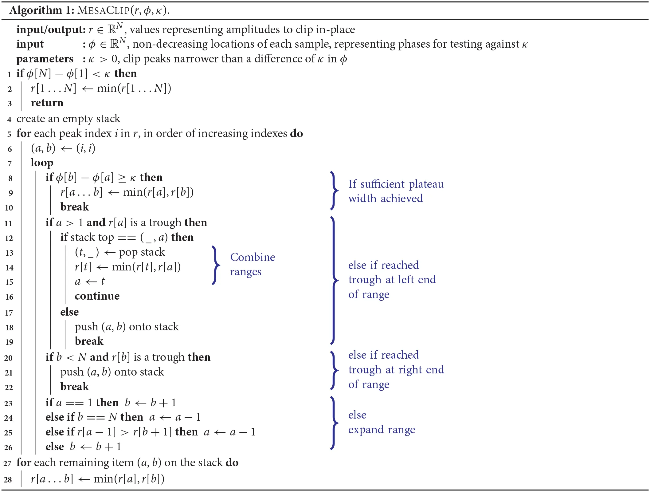
Figure 2 depicts some key moments in the execution of mesaclip, where the values of ϕ are uniformly increasing for the purpose of simplifying the illustration, but in practice they would correspond to a non-uniformly increasing phase.
Figure 2
4. Results
To illustrate the effect of the mesaclip approach compared to a conventional wavelet transform approach, Figure 3 shows three artificial signals (a-c) and one real EMG signal recorded from smooth-muscle (d). A Python implementation is available at https://github.com/lwiklendt/mesaclip.
Figure 3
We also compared the mesaclip approach to simple spike-detection based on threshold crossing, which we refer to as “peak.” The peak method works by first deciding on a threshold voltage level. Each interval of time with contiguous samples above the threshold is considered a peak. The spike time is given by the time of the maximum voltage within that peak interval. Figure 4 shows a comparison between these two approaches applied to EMG data recorded from rodent smooth muscle.
Figure 4
To explore how the mesaclip approach compares to the peak approach, we simulated signals of varying degrees of signal-to-noise ratio (SNR) and spike regularity. To generate each signal, we randomly sampled spike trains where the inverse of each inter-spike-interval (ISI) was drawn from the log-normal distribution with μ = log2(8) and . Each spike train was then rasterized into a signal with 0 where no spike occurred and 1 where a spike occurred. The signal was then Gaussian-smoothed with a width of σ = 0.01 to simulate membrane potential bumps, and a single time-sample spike was added with a noisy height drawn from 1/(1+ex) with to simulate spike-height variability. Pink noise (1/f) was added with varying degrees of SNR. For each level of regularity and SNR, 1,000 spike train signals were generated. The second and third rows of Figure 5 show examples of the spike trains and the generated signals, with the top row showing the histogram of inverse ISIs from all spike trains.
Figure 5
For each signal, the mesaclip algorithm was run and the global wavelet spectrum calculated by averaging the squared amplitudes over time. Although k = 2 is recommended, k = 4 and k = 8 have also been shown. Concurrently, the peak approach for 3-levels of threshold (with proportions 0.3, 0.5, and 0.7) between the signal's mean and its maximum were calculated, and the histogram of the inverse ISIs calculated over the same frequency domain as for the mesaclip approach. Figure 5 shows examples of the spike signals and the two frequency estimation approaches, and Figure 6 shows a comparison of errors in the frequency estimation.
Figure 6
5. Discussion
The mesaclip algorithm depends on the highly time-localized wavelet described in section 3, which results in a necessarily poorer frequency localization due to Heisenberg uncertainty (Mallat, 2008). This limitation should be taken into account with regard to the characteristics of the signal to be analyzed when deciding whether to use mesaclip, or if using mesaclip whether to apply a post-processing step to refine the frequency distribution. An analogy would be if one were to average inter-spike-intervals (ISIs) over successive time-blocks. Fewer but longer blocks would result in a tighter distribution of average ISIs, whereas a greater number of shorter blocks would result in a wider distribution of average ISIs. One could use a post-processing step to combine multiple smaller blocks to refine the averages. However, such a refinement algorithm is not covered in this paper.
The results in section 4 show how well the proposed mesaclip approach works on a variety of signals without any parameter tuning, compared to the peak approach which is highly dependent on the arbitrary choice of threshold. In particular, Figure 5 shows that the mesaclip approach works well on various signal-to-noise ratios and does not suffer from the subharmonic artifacts that the peak approach does on the simulated data. The subharmonic artifacts are due to noisy spike heights randomly falling below the chosen threshold.
Since phases are retained in the mesaclip approach, one can compute the phase-difference between two signals. Another potential approach for detecting phase-differences between two spike trains is to apply cross-correlation. However, cross-correlation is a global measure that can reveal phase-differences only in stationary signals. To apply to non-stationary signals a windowing function and choice of window size is needed. An appropriate window size depends on estimating the time scale at which the stationarity breaks down. Also, consider that phase-differences can be frequency dependent. That is, two spike trains may be offset by some phase and occur in bursts offset by a different phase that could even have opposite sign. Additionally, both subharmonic and harmonic artifacts are present in auto and cross-correlations. Accounting for all these problems and free parameters leads to a cumbersome and potentially error-prone use of cross-correlation.
The principle difference between the mesaclip and peak approaches is that the mesaclip approach is essentially an amplitude-integrated or area-under-the-curve (AUC) approach and the peak approach is an amplitude-threshold approach. The AUC of any particular spike is particularly small, and so the spikes themselves have a small contribution to the result, and we rely on the underlying membrane-potential to inform the frequencies. If the underlying membrane-potential is a poor representation of the activity one wishes to observe, for example, if there is a relatively low-amplitude but high-powered oscillating artifact together with high-amplitude but low-powered spikes, then with the mesaclip approach the oscillating artifact will drown-out the spikes. In this case, if the oscillating artifact cannot be filtered out then a peak approach should be considered instead. If the spikes are very clear (as in Figure 3D), then the peak approach is simpler and may be sufficient.
6. Conclusion
An algorithm for the removal of high-frequency artifacts from the amplitudes of a wavelet transform was presented. The artifacts are a result of non-sinusoidal oscillations characterized as spikes of short duration or sharp edges, separated by longer intervals. The algorithm removes these artifacts by inspecting the phase differences of wavelet amplitudes and clipping their amplitudes when the phase differences are shorter than a specified number of cycles. This results in a considerable proportion of the remaining amplitudes pertaining to the intervals between spikes, allowing clearer identification of the frequencies at which events occur.
The proposed approach: (1) contains no free parameters beyond k which is application-dependent, recording-independent, and due to the excellent default k = 2 could be considered to have no free parameters; (2) allows one to obtain phase differences at each frequency; (3) the time-window over which the signal's instantaneous information is integrated is optimal for each frequency; (4) is not susceptible to subharmonic artifacts; (5) the potential problem of harmonic artifacts have now been solved with the presented mesaclip algorithm.
Statements
Data availability statement
The datasets generated for this study are available on request to the corresponding author.
Ethics statement
The animal study was reviewed and approved by Animal Welfare Committee of Flinders University #861-13.
Author contributions
LW wrote the entire software development, the manuscript, and devised the methodology. LT performed the experiments and selected the pertinent recordings. All the other authors helped to write and review, and establish the concepts presented.
Conflict of interest
The authors declare that the research was conducted in the absence of any commercial or financial relationships that could be construed as a potential conflict of interest.
Footnotes
1.^Such a mapping does not exist in general due to instantaneous frequencies of 0, but we can work around this by treating ϕ(φ′) as a fiber and later replacing r(ϕ(φ′))≥h with {t ∈ ϕ(φ′) | r(t)≥h}≠∅.
References
1
AdamsR. P.MurrayI.MacKayD. J. (2009). Tractable nonparametric bayesian inference in poisson processes with gaussian process intensities, in Proceedings of the 26th Annual International Conference on Machine Learning (Montreal, QC: ACM), 9–16. 10.1145/1553374.1553376
2
BloomfieldD. S.McAteerR. J.LitesB. W.JudgeP. G.MathioudakisM.KeenanF. P. (2004). Wavelet phase coherence analysis: application to a quiet-sun magnetic element. Astrophys. J. 617:623. 10.1086/425300
3
DaubechiesI.LuJ.WuH. T. (2011). Synchrosqueezed wavelet transforms: an empirical mode decomposition-like tool. Appl. Comput. Harmon. Anal. 30, 243–261. 10.1016/j.acha.2010.08.002
4
EhrentreichF.SümmchenL. (2001). Spike removal and denoising of raman spectra by wavelet transform methods. Anal. Chem. 73, 4364–4373. 10.1021/ac0013756
5
FargeM. (1992). Wavelet transforms and their applications to turbulence. Annu. Rev. Fluid Mech. 24, 395–458. 10.1146/annurev.fl.24.010192.002143
6
GrinstedA.MooreJ. C.JevrejevaS. (2004). Application of the cross wavelet transform and wavelet coherence to geophysical time series. Nonlin. Process. Geophys. 11, 561–566. 10.5194/npg-11-561-2004
7
LewickiM. S. (1998). A review of methods for spike sorting: the detection and classification of neural action potentials. Netw. Comput. Neural Syst. 9, R53–R78. 10.1088/0954-898X_9_4_001
8
LillyJ. M.OlhedeS. C. (2009). Higher-order properties of analytic wavelets. IEEE Trans. Signal Process. 57, 146–160. 10.1109/TSP.2008.2007607
9
LillyJ. M.OlhedeS. C. (2012). Generalized morse wavelets as a superfamily of analytic wavelets. IEEE Trans. Signal Process. 60, 6036–6041. 10.1109/TSP.2012.2210890
10
LinC. Y.SuL.WuH. T. (2018). Wave-shape function analysis. J. Fourier Anal. Appl.24, 451–505. 10.1007/s00041-017-9523-0
11
MallatS. (2008). A Wavelet Tour of Signal Processing: The Sparse Way. Montreal, QC: Academic Press.
12
NenadicZ.BurdickJ. W. (2005). Spike detection using the continuous wavelet transform. IEEE Trans. Biomed. Eng. 52, 74–87. 10.1109/TBME.2004.839800
13
TorrenceC.CompoG. P. (1998). A practical guide to wavelet analysis. Bull. Am. Meteorol. Soc. 79, 61–78. 10.1175/1520-0477(1998)079<0061:APGTWA>2.0.CO;2
14
TorrenceC.WebsterP. J. (1999). Interdecadal changes in the enso-monsoon system. J. Clim. 12, 2679–2690. 10.1175/1520-0442(1999)012<2679:ICITEM>2.0.CO;2
15
VeneriG.FederighiP.RosiniF.FedericoA.RufaA. (2011). Spike removal through multiscale wavelet and entropy analysis of ocular motor noise: a case study in patients with cerebellar disease. J. Neurosci. Methods196, 318–326. 10.1016/j.jneumeth.2011.01.006
Summary
Keywords
artifact removal, non-harmonic model, action potential, wavelet transform, time-frequency analysis
Citation
Wiklendt L, Brookes SJH, Costa M, Travis L, Spencer NJ and Dinning PG (2020) A Novel Method for Electrophysiological Analysis of EMG Signals Using MesaClip. Front. Physiol. 11:484. doi: 10.3389/fphys.2020.00484
Received
12 November 2019
Accepted
20 April 2020
Published
09 June 2020
Volume
11 - 2020
Edited by
Felix Viana, Institute of Neurosciences of Alicante (IN), Spain
Reviewed by
Alex Reyes, New York University, United States; Salvador Sala, Universidad Miguel Hernández de Elche, Spain
Updates
Copyright
© 2020 Wiklendt, Brookes, Costa, Travis, Spencer and Dinning.
This is an open-access article distributed under the terms of the Creative Commons Attribution License (CC BY). The use, distribution or reproduction in other forums is permitted, provided the original author(s) and the copyright owner(s) are credited and that the original publication in this journal is cited, in accordance with accepted academic practice. No use, distribution or reproduction is permitted which does not comply with these terms.
*Correspondence: Lukasz Wiklendt lukasz.wiklendt@flinders.edu.au
This article was submitted to Autonomic Neuroscience, a section of the journal Frontiers in Physiology
Disclaimer
All claims expressed in this article are solely those of the authors and do not necessarily represent those of their affiliated organizations, or those of the publisher, the editors and the reviewers. Any product that may be evaluated in this article or claim that may be made by its manufacturer is not guaranteed or endorsed by the publisher.