 Sansao A. Pedro1
 Frank T. Ndjomatchoua2
 Peter Jentsch3,4
 Jean M. Tchuenche5
 Madhur Anand3
 Chris T. Bauch4*
- 1Departamento de Matemática e Informática, Universidade Eduardo Mondlane, Maputo, Mozambique
- 2Sustainable Impact Platform, Geospatial Science and Modelling Cluster, International Rice Research Institute, Metro Manila, Philippines
- 3School of Environmental Sciences, University of Guelph, Guelph, ON, Canada
- 4Department of Applied Mathematics, University of Waterloo, Waterloo, ON, Canada
- 5Avenir Health, Glastonbury, CT, United States
In May 2020, many jurisdictions around the world began lifting physical distancing restrictions against the spread of severe acute respiratory syndrome coronavirus 2 (SARS-CoV-2). This gave rise to concerns about a possible second wave of coronavirus disease 2019 (COVID-19). These restrictions were imposed in response to the presence of COVID-19 in populations, usually with the broad support of affected populations. However, the lifting of restrictions is also a population response to the accumulating socio-economic impacts of restrictions, and lifting of restrictions is expected to increase the number of COVID-19 cases, in turn. This suggests that the COVID-19 pandemic exemplifies a coupled behavior-disease system where disease dynamics and social dynamics are locked in a mutual feedback loop. Here we develop a minimal mathematical model of the interaction between social support for school and workplace closure and the transmission dynamics of SARS-CoV-2. We find that a second wave of COVID-19 occurs across a broad range of plausible model input parameters governing epidemiological and social conditions, on account of instabilities generated by behavior-disease interactions. The second wave tends to have a higher peak than the first wave when the efficacy of restrictions is greater than 40% and when the basic reproduction number R0 is less than 2.4. Surprisingly, we also found that a lower R0 value makes a second wave more likely, on account of behavioral feedback (although a lower R0 does not necessarily cause more infections, in total). We conclude that second waves of COVID-19 can be interpreted as the outcome of non-linear interactions between disease dynamics and social behavior. We also suggest that further development of mathematical models exploring behavior-disease interactions could help us better understand how social and epidemiological conditions together determine how pandemics unfold.
1. Introduction
The COVID-19 pandemic has given rise to an “epidemic of models” [1]. Diverse mathematical models of SARS-CoV-2 transmission (the virus that causes COVID-19 disease) have been instrumental in capturing infection dynamics and informing public health control efforts to mitigate the COVID-19 pandemic and reduce the mortality rate. The concept of “flattening the curve” comes from model outputs that show how reducing the transmission rate through efforts such as contact tracing and physical distancing can lower and delay the epidemic peak [2].
On account of limited options for pharmaceutical interventions such as vaccines, and inadequate testing capacity in many jurisdictions, the COVID-19 pandemic has also been characterized by large-scale physical distancing efforts–including school and workplace closure–being adopted by entire populations despite heavy economic costs. Mathematical models of SARS-CoV-2 transmission and control show that physical distancing can mitigate the pandemic [2–5] and this has subsequently been backed up by empirical analyses of case notification data. These analyses show how mitigation measures have reduced the effective reproduction number of SARS-CoV-2 below one, meaning that each infected case infects less than one person on average [6–8]. However, the population's willingness to support school and workplace closures could wane over time, as the economic costs of closure accumulate [9]. This has given rise to the possibility of a second wave of COVID-19 in many populations.
The large role played by physical distancing during the COVID-19 pandemic exemplifies a coupled behavior-disease system, in which human behavior influences infectious disease transmission and vice versa [10–16]. These systems are part of a broader class of pervasive systems in which human behavior both influences, and responds to, the dynamics of our environment. Hence, one might better speak of a single, coupled human-environment system, instead of just human systems or environmental systems in isolation from one another [17–19].
The interactions between disease dynamics and behavioral dynamics in COVID-19 are emphasized by research showing that the perceived risk of SARS-CoV-2 infection is a predictor of adherence to physical distancing measures [20] and moreover that individuals respond to the presence of COVID-19 cases in their population by increasing their physical distancing efforts [21]. In turn, physical distancing has been shown to reduce the number of cases [6], completing the loop of coupled behavior-disease dynamics. Some models have already begun exploring this interaction between disease dynamics and individual behavior and/or public health policy decision-making for COVID-19 [5, 16, 22–26]. The emergence of a second wave of COVID-19 on account of population attitudes to physical distancing has also been explored in mathematical models [27].
The social aspects of behavior-disease interactions seem to be relevant for COVID-19 decision-making. Individuals do not necessarily make the best possible (most rational) response to the presence of COVID-19 cases in their population. Instead, it has been found that political leaders can be influential in convincing individuals to change their physical distancing efforts [23]. Additionally, jurisdictions experiencing outbreaks that start relatively late appear to learn from the experiences of jurisdictions that were affected earlier [28]. Meanwhile, other research emphasizes a need for more work on the socio-economic aspects of the pandemic [29]. These findings suggest that imitation and social learning processes are important for understanding interactions between disease dynamics and decision-making for COVID-19, which ultimately determine the epidemic curve.
Here we model the coupled behavior-disease dynamics of SARS-CoV-2 transmission and population support for school and workplace closure, using a simplified theoretical model. We opted for a simple model that avoids heterogeneities because our objective is to gain insights into potential interactions between social and behavioral dynamics. Public opinion evolves according to social learning rules [10, 18], and public opinion in support of closure depends both on COVID-19 case incidence and accumulated socio-economic losses due to school and workplace closure. A central decision-maker chooses a time to initially close schools and workplaces when the outbreak begins, but may subsequently open and close them again depending on how public opinion ebbs and flows. Meanwhile, disease dynamics are described by a compartmental epidemic model [30]. The details of our mathematical model are described in the section 2. We analyze the model to characterize the conditions that give rise to a second wave of COVID-19 in the population.
2. Methods
2.1. Model Equations
Transmission dynamics are given by an SEIR model, modified to take physical distancing into account,
where S is the proportion of susceptible individuals (“susceptible”), E is the proportion of individuals who have been infected but are not yet infectious (“exposed”), I is the proportion of individuals who are both infected and infectious (“infectious”), and R is the proportion of individuals who are no longer infectious (“removed”). The time-varying parameter C(t) captures the impact of school and workplace closure on the transmission of SARS-CoV-2. β is the baseline transmission rate in the absence of school/workplace closure, σ is the time rate at which an exposed person becomes infections, and γ is the time rate at which an infectious person recovers. We use an SEIR model since they are appropriate for population-level modeling epidemics of acute, self-limiting infections that confer natural immunity [30, 31]. Since our focus is on physical distancing and lockdown, we do not include compartments for testing, contact tracing and asymptomatic transmission.
The decision-maker decides to “turn on” closure at some time tclose, and then decides to “turn off” closure when population support for closure, x(t) drops below 50%. Hence C(t) is given by:
where C0 is a combined measure of how many workplaces are closed (the remainder being essential workplaces such as hospitals) as well as the effectiveness of physical distancing in those workplaces that remain open.
Approaches to modeling human opinions and decision-making vary greatly and include agent-based network models based on complex systems science [32–34], evolutionary game theory (imitation dynamics) [10, 11, 13], mathematical models based on psychological theory [35] and other approaches. For our study system, the imitation dynamic approach is suitable because (1) imitation dynamics are sufficient to describe the population-level opinion dynamics when individuals learn from one another and response to changes in their utility functions, as epidemic and socio-economic conditions evolve [36]; (2) differential equations are usually easier to analyze (either rigorously or through numerical analysis) than agent-based models. The percentage of the population that supports school and workplace closure, x, evolves according to an imitation dynamic as:
where κ is the social learning rate, ω is sensitivity to infection prevalence, and ϵ is sensitivity to accumulated socio-economic losses L. Support for closure goes up when the prevalence of infection goes up, but it declines when the accumulated socio-economic losses, L, become too large. The quadratic term x(1 − x) represents a social learning dynamics where individuals sample others at some rate, and they change opinion based on the utility difference ωI − ϵL (A full derivation of this type of differential equation appears in [18]). The social learning rate κ represents how often individuals discuss opinions about lockdown. The parameter ω control how the population opinion about lockdown reacts to the prevalence of infection, and it is influenced by the perceived risk of the severity of infection (frequency of severe cases, hospitalizations, and deaths). The parameter ϵ controls how population opinion about lockdown reacts to socio-economic losses and is influenced by the perception of how severe the socio-economic losses as a function of media coverage, for instance.
We can absorb ω into κ, yielding:
and then, setting κ′ = κω and ϵ′ = ϵ/ω and dropping the primes for simplicity we obtain
Finally, the variable L is a phenomenological representation of accumulated socio-economic losses obeying
where α controls the rate at which school and workplace closure impacts socio-economic health of the population, and δ is a decay rate that represents adjustment to baseline losses. These two parameters represent the sum effect of multiple processes. For instance, α is influenced by what proportion of workers are affected by lockdown through loss of employment or working hours; household savings and debt; and economic stimulus packages. Similarly, δ is determined by economic discounting, the ability of individuals to adjust to new economic circumstances (for instance by offering new products and services to meet demand in a pandemic market), and other factors.
2.2. Parameterization
A full list of parameter definitions, baseline values, and literature sources appears in Table 1. The transition rates σ and γ, were set based on COVID-19 epidemiological literature [37–39, 44, 45], while the transmission rate β was estimated. Note that the last compartment of the model, R, does not correspond to a stage of illness preceding recovery but rather a stage of infectiousness [31], which wanes quickly after the imposition of case isolation, in addition to the decline in viral shedding after the first 5 days [46]. Moreover, the infectious stages is preceded by a latent stage in which the virus is still replicating inside its new host until it can reach a level where the host can transmit the infection to others. These features of COVID-19 disease history guided our choice of γ and σ. Since the prevalence I(t) as used in the model is different from case incidence as appears in daily lab-confirmed case reports, a new state variable denoting daily infection incidence, Ii was defined as the difference between accumulated health outcomes. That is, Ii(t) = H(t) − H(t − 1), where H(t) is the cumulative number of cases at time t:
The state variable Ii(t) was used when fitting the model to daily case notifications was required.
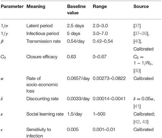
Table 1. Parameter values, baseline values, and literature sources.
Because ϵ, κ, and α and ω encapsulate many different factors, we take the approach of inferring parameter values by fitting the model to data. (We also explore the impact of variation in these parameter values in sensitivity analysis through parameter planes). To avoid over-fitting, δ is fixed based on commonly used discounting rates. The social parameters κ and ϵ were calibrated. While κ dictates how quickly population opinion changes, ϵ dictates how sensitive the population is to changes in case reports relative to socio-economic losses. κ was estimated from behavior early in the epidemic when socio-economic losses are small as dx/dt ≈ κx(1 − x)I. We derived I(t) from reports of confirmed positive cases from the early stages of the United States epidemic, adjusted by a case under-ascertainment factor of 8.7 in the United States [42]. We used 21 January 2020 as the initial date of the epidemic, when the first case of COVID-19 was reported in the United States. Most populations rapidly adopted physical distancing measures against COVID-19. Gallup polls indicate that 59%/79%/92% of the United States public avoided going to events with large crowds, as of 13-15 March/16-18 March/20-22 March 2020 respectively [43]. Similarly, 30%/54%/72% avoided public places, and 23/46/68% avoided small gatherings [43]. Taking the average of these responses across the three question types, we obtain that x(52) = 0.373, x(59) = 0.597, x(66) = 0.773 where time is measured in days since January 21. Finally, we shifted these points forward 14 days as physical distancing at time t will not be reflected in infection data until t + 14 due to the delays in testing and symptom recognition. We assumed x(0) = 0.25 when fitting to these three data points using least-squares error minimization for the κ estimation.
To estimate β we used least-squares error minimization to fit the modeled Ii(t) to lab-confirmed daily case reports in the United States from the early epidemic [40]. The fitted infection trajectory, Ii is in good agreement with reported cases in the US during the initial phase of the epidemic leading up to 4 April 2020 (Supplementary Figure 1b). Our inferred estimate β = 0.54/day yields a basic reproduction number R0 ≈ β/γ = 2.7 [30], which agrees well with published estimates of R0 for SARS-CoV-2 [47]. For the special case where there is an absence of any control measures, the model predicts that about 80% of the population becomes infected by the end of the outbreak (Supplementary Figure 1a).
The remaining two parameters, ϵ and α, were calibrated to obtain the result that x remains high after the initial surge in support for closure, but begins to drop after 2 months. This period of time was based on the observation that 2 months that have elapsed since the declaration of the national emergency in the United States on 13 March 2020, and the process of re-opening state economies that has unfolded over the month of May 2020. These two parameters control the timescale of lifting school and workplace closure based on its socio-economic impacts. Finally, the parameter δ was set such that δ = 0.05α on the basis of commonly used discounting rates in economics and assuming that economic losses accumulated through the αC(t) term would be discounted at a rate of 5% per year [41].
In order to illustrate curve flattening and show that the model has the expected response to reduction in the transmission rate due to closure, we generated model timeseries of I(t) for the special case where closure is applied throughout the entire outbreak. The epidemic curve for different values of the closure efficacy C0 is shown, ranging from C0 = 0 (no intervention) to C0 = 0.6 (Supplementary Figure 1c). The timeseries show that the epidemic curve is flattened and delayed as closure becomes more efficacious, which reduces peak demand for intensive care beds and buys time for developing pharmaceutical interventions like vaccines and antiviral drugs, improving testing capacity, and establishing novel approaches to patient care. For the remainder of our analysis, to determine C0 it was assumed that C0 should be large enough to bring the effective reproduction number Reff below 1, reflecting the observed success in multiple jurisdictions where physical distancing and closure have maintained Reff < 1 [6–8]. Hence we chose C0 = 1 − 1/R0 based on the elimination threshold for the SEIR model [30]. We also assumed tclose = 20 days but in practice, our second requirement that x ≥ 50% was not reached until after 20 days in all of the model simulations. We analyzed numerical simulations of our model to determine the conditions where one or more waves of SARS-CoV-2 infections could occur. A wave was defined as a local maximum in the prevalence I(t), and the simulation time horizon was 730 days (2 years).
3. Results
3.1. Mechanisms Causing a Second Wave
At our baseline parameter values, time series of infection prevalence I(t) and support for closure x(t) exhibit non-trivial time evolution, including a second wave of COVID-19 infections (Figure 1). These results illustrate the basic mechanisms underlying the model dynamics. As infection prevalence grows, support for closure rises and eventually crosses the 50% threshold by t = 80 days. After this, infection prevalence peaks and begins to decline. Support remains at a high plateau for a period of 2 months. After this period, infection prevalence remains small while the socio-economic impacts of lockdown continued to mount. This causes waning of support for lockdown, and hence restrictions are lifted by t = 160 days. Shortly thereafter, prevalence begins to rise again. Support for closure correspondingly rises again, but not quickly enough to prevent a second wave of COVID-19 with a peak at t = 240 days that is higher than the peak of the first wave.
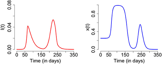
Figure 1. Second wave of COVID-19: time series plot of the number of infected individuals (left) and proportion of individuals practicing physical distancing (right). The results are obtained for C0 = 0.63, R0 = 2.675, 1/σ = 2.5, γ = 1/5, κ = 5, ϵ = 0.008, α = 1.0*24/365, and δ = 0.05*24.0/365 and initial conditions S(0) = 1 − 1/1000000, E(0) = 0, I(0) = 1/1000000, R(0) = 0, x(0) = 0.25, L(0) = 0, and H(0) = 0.
3.2. Epidemiological Conditions for a Second Wave
Our goal was to gain insight into the conditions that generate a second wave of COVID-19, and to test the robustness of the predicted result at our baseline parameter values illustrate in Figure 1. Hence we explored the model dynamics in the neighborhood of our baseline parameter values (Table 1) using parameter planes that show how the dynamical regimes of the model vary with changes in two model parameters (one on each axis) around the baseline values. We explored two dynamical outcomes: the number of waves in the course of the entire pandemic, and the ratio of the peak height of the second wave to the peak height of the first wave.
We start by exploring the effects of variation in the epidemiological parameters β (transmission rate) and γ (inverse of the average duration of infectiousness) in Figure 2, while keeping the rest of the parameters at baseline values. The results show that one, two, or three waves are possible under variation in these parameter values. A second wave characterizes most of the β − γ plane, however. A third wave appears when 1/γ is between 5 and 7 days and β is up to 0.4/day, corresponding to R0 < 2 (we note that most estimates place R0 > 2 for SARS-CoV-2 [47, 48]). The second peak may be higher or lower than the first peak, depending on the β and γ parameter combinations. For R0 > 2.4, the second peak tends to be lower than the first, while for R0 < 2.4 is higher.
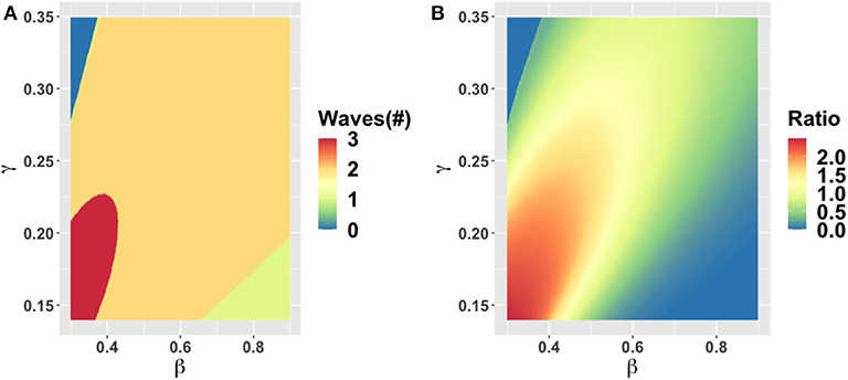
Figure 2. Parameter plane showing model dynamics as they vary with changes in the transmission rate β and the rate γ at which the infectious period ends, for the number of COVID-19 waves (A) and the ratio of peak height of the second wave to the first wave peak (B). Other parameters are at baseline values (Table 1).
The increase in the number of waves with a decrease in β (or equivalently, a decrease in the basic reproduction number R0) is notable and surprising. The classical SEIR model without behavior shows the opposite effect: increasing R0 when the endemic equilibrium is stable causes damped oscillations to be sustained for a longer period before the oscillations die down. Our model shows different dynamics than the classical SEIR model on account of strong behavioral feedback. When R0 is sufficiently high, the infection can pass through the population rapidly and cause a large amount of herd immunity to build up before the population response causes a late dampening of the epidemic curve. As a result of herd immunity, a second wave is not possible. But when R0 is smaller, the spread of SARS-CoV-2 is slow enough to allow a timely population response that flattens the curve and ends the first wave. After the first wave, cases are low, but so is herd immunity. In the meantime, the economic consequences of lockdown continue to build, causing a waning of support for continued lockdown, which in turns sparks a second wave among the remaining susceptible individuals. This process can be repeated in third and subsequent waves for some parameter values. But we emphasize that multiple waves do not necessarily correspond to more COVID-19 cases overall.
Changes in the duration of infectiousness 1/γ and the duration of the latent stage 1/σ around baseline values do not change the number of peaks: a second wave is still observed across the range we explored (Supplementary Figure 2). However, the second peak is higher than the first when 1/γ is between 3 to 5 days, while out of this range the second peak is lower. The lack of dependence of dynamics on σ is expected. When 1/γ < 3 days, the second peak is less severe because R0 drops below levels that are feasible for continued transmission in the population. In contrast, when 1/γ > 5 days the second peak is less severe because a heightened R0 causes rapid build-up of herd immunity in the first wave of infection.
3.3. Socio-Economic and Intervention Conditions for a Second Wave
Next we explored the effect of variation in intervention, economic and social parameters. The parameter plane for α, the rate at which economic losses due to closure accumulate, and δ, the discounting rate for losses, shows little variation in these values across the ranges we explored (Supplementary Figure 3). Two waves are predicted and the peak of the second wave is higher than the first wave for almost all parameter combinations. The only exception is that when α is very small, only a single wave occurs because the population is willing to tolerate economic losses indefinitely. As a result, x remains high over the entire time horizon of the simulation and COVID-19 is effectively controlled throughout this period.
The behavioral parameter κ is a measure of how quickly novel social behavior spreads through a population as disease cases are reported. It has a large influence on the model dynamics, as represented in the κ − α, κ − ϵ, and κ − C0 parameter planes (Figures 3–5). Higher values of κ indicate that individuals imitate more quickly. At our baseline value κ = 5/day, we observe a second wave. As the value of κ increases from this baseline value, the number of waves increases from two to six or seven in all three parameter planes, unless the effectiveness of closure (C0) is so low that the population experiences a single large epidemic that rapidly confers herd immunity to everyone (Figures 3–5). As κ is reduced sufficiently from its baseline value, the second wave is lost as expected, since we enter a parameter regime where the population responds with an unrealistic slowness to the presence of COVID-19, and it experiences a single, rapid pandemic wave that rapidly confers herd immunity. The second peak is higher than the first peak in all three parameter planes, except again when C0 is too low to effectively flatten the curve, and a single large outbreak results. Some examples of model outcomes for three or more waves are shown in Supplementary Figure 4. In these extreme scenarios, the second wave can either dominate the first and third waves, or it is also possible that the peaks of successive epidemic waves increase over time until it reaches a maximum peak in the fourth wave.
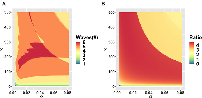
Figure 3. Parameter plane showing model dynamics as they vary with changes in the rate α at which socio-economic losses accrue and the rate κ that controls the social learning rate, for the number of COVID-19 waves (A) and the ratio of peak height of the second wave to the first wave peak (B). Other parameters are at baseline values (Table 1).
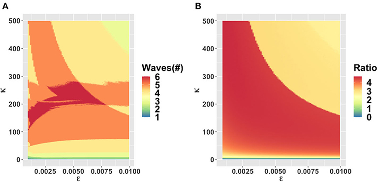
Figure 4. Parameter plane showing model dynamics as they vary with changes in the rate κ that controls the social learning rate and the parameter ϵ which controls how sensitive the population is to economic losses relative to infection prevalence, for the number of COVID-19 waves (A) and the ratio of peak height of the second wave to the first wave peak (B). Other parameters are at baseline values (Table 1).
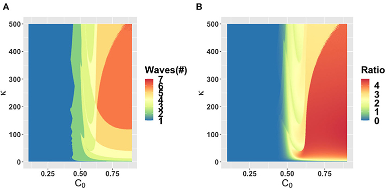
Figure 5. Parameter plane showing model dynamics as they vary with changes in the rate κ that controls the social learning rate and the parameter C0 which controls how effective closure is, for the number of COVID-19 waves (A) and the ratio of peak height of the second wave to the first wave peak (B). Other parameters are at baseline values (Table 1).
4. Discussion
A second wave of COVID-19 is widely feared in 2020 as many jurisdictions around the world begin lifting restrictions that have held viral transmission in check. To address this issue, we analyzed a simple theoretical model of the interplay between SARS-CoV-2 transmission dynamics and social dynamics concerning public support for physical distancing and school and workplace closure. We found that a second wave of COVID-19 (and sometimes also a third wave) was likely across a broad range of epidemiological and behavioral parameters. In some cases, the second peak was higher than the first peak, while for other parameter combinations it was lower.
Our prediction of a second wave driven by behavior-disease interactions is plausible, given past and recent experience with novel emerging pathogens. One of the first affected countries in the COVID-19 pandemic (Iran) is now experiencing a large second wave on account of lifting restrictions in April 2020 [49]. During the 2003 SARS-CoV-1 epidemic in Toronto, premature relaxation of control measures resulted in a second outbreak that was as large as the first outbreak [50]. Finally, behavioral responses to disease dynamics appear to have played a role in shaping the three waves that some populations experienced during the “Spanish flu” pandemic in 1918 [51].
Our model makes simplifying assumptions that could influence its projections. For instance, our model assumes that populations respond to infection prevalence I(t) but in fact, populations observe reported cases and deaths, both of which are delayed compared to time of actual infection. Time delays tend to destabilize dynamics in epidemic models [31] and hence we suspect that a model extension including a response to lagged outcomes like reported cases and deaths would exacerbate the severity of second waves in our model.
On the other hand, adding real-world spatial and demographic heterogeneities to our model could stabilize the dynamics and make the predicted oscillations less extreme, even if they do not remove them completely [52–56]. Similarly, on the behavioral modeling side, we suggest that the extreme oscillations observed in this model could also be stabilized if individuals use past and/or projected future states in their decision-making, instead of just the current prevalence, as we assumed [57, 58]. Alternatively, if individuals learn socially from other populations at differing stages of COVID-19 outbreaks [28], and not just their local population, this might also dampen the oscillations we observed in the model.
In summary, we speculate that incorporating social and spatial heterogeneities into the model would not completely remove the possibility of a second wave, although it could dampen the cycles [52–56] and give rise to epidemic curves more closely resembling that observed in the second wave in Iran [49]. Moreover, our prediction of a second wave was relatively robust across parameter space. Hence, we conclude that a second wave of COVID-19 on account of the coupled behavior-disease feedbacks we explore in this model will characterize many populations. Because interactions between the dynamics of disease spread and social processes will play a major role in shaping the pandemic, more effort in transmission modeling of COVID-19 should be devoted to accounting for them.
Data Availability Statement
The original contributions presented in the study are included in the article/Supplementary Material, further inquiries can be directed to the corresponding author/s.
Author Contributions
CB, MA, and JT conceived the study. SP and FN conducted the research. All authors developed the model and analysis and wrote the manuscript.
Funding
This research was funded by NSERC Discovery Grants and an Ontario Ministry of College and Universities grant to CB and MA. SP was partially supported by Program UEM-SIDA 2017-2022 under the Subprogramme Nr 1.4.2: Capacity Building in Mathematics, Statistics and Its Applications.
Conflict of Interest
The authors declare that the research was conducted in the absence of any commercial or financial relationships that could be construed as a potential conflict of interest.
Acknowledgments
The authors are grateful to comments from two reviewers. This manuscript has been released as a pre-print at medRxiv [59].
Supplementary Material
The Supplementary Material for this article can be found online at: https://www.frontiersin.org/articles/10.3389/fphy.2020.574514/full#supplementary-material
References
1. Yan P. Non-identifiables and invariant quantities in infectious disease models. In: Mathematical Understanding of Infectious Disease Dynamics. Singapore: World Scientific (2009). p. 167-229. doi: 10.1142/9789812834836_0005
2. Tuite AR, Fisman DN, Greer AL. Mathematical modelling of COVID-19 transmission and mitigation strategies in the population of Ontario, Canada. CMAJ. (2020) 192:E497–505. doi: 10.1101/2020.03.24.20042705
3. Kucharski AJ, Klepac P, Conlan A, Kissler SM, Tang M, Fry H, et al. Effectiveness of isolation, testing, contact tracing and physical distancing on reducing transmission of SARS-CoV-2 in different settings. medRxiv [Preprint]. (2020). doi: 10.1101/2020.04.23.20077024
4. Roosa K, Lee Y, Luo R, Kirpich A, Rothenberg R, Hyman J, et al. Real-time forecasts of the COVID-19 epidemic in China from February 5th to February 24th, 2020. Infect Dis Modell. (2020) 5:256–63. doi: 10.1016/j.idm.2020.02.002
5. Karatayev VA, Anand M, Bauch CT. “Local lockdowns outperform global lockdown on the far side of the COVID-19 epidemic curve.” In Proceedings of the National Academy of Sciences. (2020)
6. Dreher N, Spiera Z, McAuley FM, Kuohn L, Durbin JR, Marayati NF, et al. Impact of policy interventions and social distancing on SARS-CoV-2 transmission in the United States. medRxiv [Preprint]. (2020). doi: 10.1101/2020.05.01.20088179
7. McGrail DJ, Dai J, McAndrews KM, Kalluri R. Enacting national social distancing policies corresponds with dramatic reduction in COVID-19 infection rates. medRxiv. (2020) 15:e0236619. doi: 10.1101/2020.04.23.20077271
8. Anderson SC, Edwards AM, Yerlanov M, Mulberry N, Stockdale J, Iyaniwura SA, et al. Estimating the impact of COVID-19 control measures using a Bayesian model of physical distancing. medRxiv [Preprint]. (2020). doi: 10.1101/2020.04.17.20070086
9. Brodeur A, Clark AE, Fléche S, Powdthavee N. COVID-19, Lockdowns and Well-Being: Evidence from Google Trends. Institute of Labor Economics (IZA) (2020).
10. Bauch CT. Imitation dynamics predict vaccinating behaviour. Proc R Soc B Biol Sci. (2005) 272:1669–75. doi: 10.1098/rspb.2005.3153
11. Reluga TC. Game theory of social distancing in response to an epidemic. PLoS Comput Biol. (2010) 6:e1000793. doi: 10.1371/journal.pcbi.1000793
12. Funk S, Salathé M, Jansen VA. Modelling the influence of human behaviour on the spread of infectious diseases: a review. J R Soc Interface. (2010) 7:1247–56. doi: 10.1098/rsif.2010.0142
13. Fu F, Rosenbloom DI, Wang L, Nowak MA. Imitation dynamics of vaccination behaviour on social networks. Proc R Soc B Biol Sci. (2011) 278:42–9. doi: 10.1098/rspb.2010.1107
14. Mbah MLN, Liu J, Bauch CT, Tekel YI, Medlock J, Meyers LA, et al. The impact of imitation on vaccination behavior in social contact networks. PLoS Comput Biol. (2012) 8:e1002469. doi: 10.1371/journal.pcbi.1002469
15. Bauch CT, Galvani AP. Social factors in epidemiology. Science. (2013) 342:47–9. doi: 10.1126/science.1244492
16. Zhao S, Stone L, Gao D, Musa SS, Chong MK, He D, et al. Imitation dynamics in the mitigation of the novel coronavirus disease (COVID-19) outbreak in Wuhan, China from 2019 to 2020. Ann Transl Med. (2020) 8:448. doi: 10.21037/atm.2020.03.168
17. Turner BL, Matson PA, McCarthy JJ, Corell RW, Christensen L, Eckley N, et al. Illustrating the coupled human-environment system for vulnerability analysis: three case studies. Proc Natl Acad Sci USA. (2003) 100:8080–5. doi: 10.1073/pnas.1231334100
18. Thampi VA, Anand M, Bauch CT. Socio-ecological dynamics of Caribbean coral reef ecosystems and conservation opinion propagation. Sci Rep. (2018) 8:1–11. doi: 10.1038/s41598-018-33573-x
19. Henderson KA, Bauch CT, Anand M. Alternative stable states and the sustainability of forests, grasslands, and agriculture. Proc Natl Acad Sci USA. (2016) 113:14552–9. doi: 10.1073/pnas.1604987113
20. Pollak Y, Dayan H, Shoham R, Berger I. Predictors of adherence to public health instructions during the COVID-19 pandemic. medRxiv [Preprint]. (2020). doi: 10.1101/2020.04.24.20076620
21. Yan Y, Malik AA, Bayham J, Fenichel EP, Couzens C, Omer SB. Measuring voluntary social distancing behavior during the COVID-19 pandemic. medRxiv [Preprint]. (2020). doi: 10.1101/2020.05.01.20087874
22. Rossberg AG, Knell RJ. How will this continue? Modelling interactions between the COVID-19 pandemic and policy responses. medRxiv [Preprint]. (2020). doi: 10.1101/2020.03.30.20047597
23. Ajzenman N, Cavalcanti T, Da Mata D. More than words: leaders? Speech and risky behavior during a pandemic. SSRN. (2020). doi: 10.2139/ssrn.3582908. [Epub ahead of print].
24. Kochańczyk M, Grabowski F, Lipniacki T. Dynamics of COVID-19 pandemic at constant and time-dependent contact rates. Math Modell Nat Phenomena. (2020) 15:28. doi: 10.1051/mmnp/2020011
25. Rowlett J, Karlsson CJ. Decisions and disease: the evolution of cooperation in a pandemic. arXiv[Preprint].arXiv:200412446. (2020) doi: 10.1038/s41598-020-69546-2
26. Steinegger B, Arenas A, Gómez-Gardenes J, Granell C. Pulsating campaigns of human prophylaxis driven by risk perception palliate oscillations of direct contact transmitted diseases. Phys Rev Res. (2020) 2:023181. doi: 10.1103/PhysRevResearch.2.023181
27. Johnston MD, Pell B. A dynamical framework for modeling fear of infection and frustration with social distancing in COVID-19 spread. arXiv[Preprint].arXiv:200806023. (2020).
28. Tellis GJ, Sood N, Sood A. Why did US governors delay lockdowns against COVID-19? Disease Science vs Learning, Cascades, and Political Polarization. SSRN. (2020). doi: 10.2139/ssrn.3575004. [Epub ahead of print].
29. Hossain MM. Current status of global research on novel coronavirus disease (COVID-19): a bibliometric analysis and knowledge mapping. SSRN. (2020). doi: 10.2139/ssrn.3547824. [Epub ahead of print].
30. Hethcote HW. The mathematics of infectious diseases. SIAM Rev. (2000) 42:599–653. doi: 10.1137/S0036144500371907
31. Anderson RM, May RM. Infectious Diseases of Humans: Dynamics and Control. Oxford: Oxford University Press (1992).
32. Gao C, Liu J. Modeling and restraining mobile virus propagation. IEEE Trans. Mobile Comput. (2012) 12:529–41. doi: 10.1109/TMC.2012.29
33. Gao C, Liu J. Network-based modeling for characterizing human collective behaviors during extreme events. IEEE Trans. Syst. Man Cybernet. Syst. (2016) 47:171–83. doi: 10.1109/TSMC.2016.2608658
34. Wang Z, Bauch CT, Bhattacharyya S, d'Onofrio A, Manfredi P, Perc M, et al. Statistical physics of vaccination. Phys Rep. (2016) 664:1–13. doi: 10.1016/j.physrep.2016.10.006
35. Beckage B, Gross LJ, Lacasse K, Carr E, Metcalf SS, Winter JM, et al. Linking models of human behaviour and climate alters projected climate change. Nat Clim Change. (2018) 8:79–84. doi: 10.1038/s41558-017-0031-7
36. Bauch CT, Bhattacharyya S. Evolutionary game theory and social learning can determine how vaccine scares unfold. PLoS Comput Biol. (2012) 8:e1002452. doi: 10.1371/journal.pcbi.1002452
37. Linton NM, Kobayashi T, Yang Y, Hayashi K, Akhmetzhanov AR, Jung Sm, et al. Incubation period and other epidemiological characteristics of 2019 novel coronavirus infections with right truncation: a statistical analysis of publicly available case data. J Clin Med. (2020) 9:538. doi: 10.3390/jcm9020538
38. Kucharski AJ, Russell TW, Diamond C, Liu Y, Edmunds J, Funk S, et al. Early dynamics of transmission and control of COVID-19: a mathematical modelling study. Lancet Infect Dis. (2020) 20:553–8. doi: 10.1101/2020.01.31.20019901
39. Li Q, Guan X, Wu P, Wang X, Zhou L, Tong Y, et al. Early transmission dynamics in Wuhan, China, of novel coronavirus-infected pneumonia. N Engl J Med. (2020) 382:1199-207. doi: 10.1056/NEJMoa2001316
40. Dong E, Du H, Gardner L. An interactive web-based dashboard to track COVID-19 in real time. Lancet Infect Dis. (2020) 20:533–4. doi: 10.1016/S1473-3099(20)30120-1
41. Hjelmgren J, Berggren F, Andersson F. Health economic guidelines, similarities, differences and some implications. Value Health. (2001) 4:225–50. doi: 10.1046/j.1524-4733.2001.43040.x
42. Lachmann A. Correcting under-reported COVID-19 case numbers. medRxiv [Preprint]. (2020). doi: 10.1101/2020.03.14.20036178
43. Saad L. Americans Step Up Their Social Distancing Even Further (2020). Available from: https://news.gallup.com/opinion/gallup/298310/americans-step-social-distancing-even-further.aspx
44. Park SW, Cornforth DM, Dushoff J, Weitz JS. The time scale of asymptomatic transmission affects estimates of epidemic potential in the COVID-19 outbreak. medRxiv. (2020). doi: 10.1101/2020.03.09.20033514
45. Hellewell J, Abbott S, Gimma A, Bosse NI, Jarvis CI, Russell TW, et al. Feasibility of controlling COVID-19 outbreaks by isolation of cases and contacts. Lancet Global Health. (2020). doi: 10.1101/2020.02.08.20021162
46. He X, Lau EH, Wu P, Deng X, Wang J, Hao X, et al. Temporal dynamics in viral shedding and transmissibility of COVID-19. Nat Med. (2020) 26:672–5. doi: 10.1038/s41591-020-1016-z
47. Liu Y, Gayle AA, Wilder-Smith A, Rocklöv J. The reproductive number of COVID-19 is higher compared to SARS coronavirus. J. Travel Med. (2020) 27:taaa021. doi: 10.1093/jtm/taaa021
48. Hilton J, Keeling MJ. Estimation of country-level basic reproductive ratios for novel Coronavirus (COVID-19) using synthetic contact matrices. medRxiv [Preprint]. (2020). doi: 10.1101/2020.02.26.20028167
49. Johns Hopkins Coronavirus Resource Center. (2020). Available online at: https://coronavirus.jhu.edu/ (accessed May 21, 2020).
50. News From the Centers for Disease Control and Prevention. Update: severe acute respiratory syndrome-Toronto, Canada, 2003. MMWR Morbid Mortal Weekly Rep. (2003) 52:547.
51. He D, Dushoff J, Day T, Ma J, Earn DJ. Inferring the causes of the three waves of the 1918 influenza pandemic in England and Wales. Proc R Soc B Biol Sci. (2013) 280:20131345. doi: 10.1098/rspb.2013.1345
52. Grenfell BT, Kleczkowski A, Gilligan C, Bolker B. Spatial heterogeneity, nonlinear dynamics and chaos in infectious diseases. Stat Methods Med Res. (1995) 4:160–183. doi: 10.1177/096228029500400205
53. Lloyd AL, May RM. Spatial heterogeneity in epidemic models. J Theor Biol. (1996) 179:1–11. doi: 10.1006/jtbi.1996.0042
54. Earn DJ, Rohani P, Grenfell BT. Persistence, chaos and synchrony in ecology and epidemiology. Proc R Soc Lond Ser B Biol Sci. (1998) 265:7–10. doi: 10.1098/rspb.1998.0256
55. Viboud C, Bjornstad ON, Smith DL, Simonsen L, Miller MA, Grenfell BT. Synchrony, waves, and spatial hierarchies in the spread of influenza. Science. (2006) 312:447–51. doi: 10.1126/science.1125237
56. Metcalf CJE, Hampson K, Tatem AJ, Grenfell BT, Bjornstad ON. Persistence in epidemic metapopulations: quantifying the rescue effects for measles, mumps, rubella and whooping cough. PLoS ONE. (2013) 8:e74696. doi: 10.1371/journal.pone.0074696
57. Wells CR, Bauch CT. The impact of personal experiences with infection and vaccination on behaviour-incidence dynamics of seasonal influenza. Epidemics. (2012) 4:139–51. doi: 10.1016/j.epidem.2012.06.002
58. Bury TM, Bauch CT, Anand M. Charting pathways to climate change mitigation in a coupled socio-climate model. PLoS Comput Biol. (2019) 15:e1007000. doi: 10.1371/journal.pcbi.1007000
Keywords: COVID-19, epidemic model, behavioral fatigue, coupled behavior-disease system, SARS-CoV-2, evolutionary game theory, imitation dynamics, social learning
Citation: Pedro SA, Ndjomatchoua FT, Jentsch P, Tchuenche JM, Anand M and Bauch CT (2020) Conditions for a Second Wave of COVID-19 Due to Interactions Between Disease Dynamics and Social Processes. Front. Phys. 8:574514. doi: 10.3389/fphy.2020.574514
Received: 20 June 2020; Accepted: 27 August 2020;
Published: 09 October 2020.
Edited by:
Zhanwei Du, University of Texas at Austin, United StatesCopyright © 2020 Pedro, Ndjomatchoua, Jentsch, Tchuenche, Anand and Bauch. This is an open-access article distributed under the terms of the Creative Commons Attribution License (CC BY). The use, distribution or reproduction in other forums is permitted, provided the original author(s) and the copyright owner(s) are credited and that the original publication in this journal is cited, in accordance with accepted academic practice. No use, distribution or reproduction is permitted which does not comply with these terms.
*Correspondence: Chris T. Bauch, Y2JhdWNoQHV3YXRlcmxvby5jYQ==