 Aaron Held
- Theoretical Physics, Blackett Laboratory, Imperial College London, London, United Kingdom
Effective field theory provides a new perspective on the predictive power of Renormalization Group fixed points. Critical trajectories between different fixed points confine the regions of UV-complete, IR-complete, as well as conformal theories. The associated boundary surfaces cannot be crossed by the Renormalization Group flow of any effective field theory. We delineate cases in which the boundary surface acts as an infrared attractor for generic effective field theories. Gauge-Yukawa theories serve as an example that is both perturbative and of direct phenomenological interest. We identify additional matter fields such that all the observed coupling values of the Standard Model, apart from the Abelian hypercharge, lie within the conformal region. We define a quantitative measure of the predictivity of effective asymptotic safety and demonstrate phenomenological constraints for the associated beyond Standard-Model Yukawa couplings.
1. Motivation
Effective field theory (EFT) describes all of high-energy physics remarkably well—see [1] for a review of Standard Model (SM) EFT, and [2] for a well-defined EFT of gravity below the Planck scale. EFTs are solely governed by their field content and symmetries (both global and local). The theory space of all possible realizations of an EFT is spanned by the couplings associated with the (infinite) set of all independent symmetry invariants. A specific realization is characterized by its coupling values at some Renormalization Group (RG) scale. Despite the infinitely many couplings, perturbative and local EFTs are predictive toward the infrared (IR) since the infinite tower of higher-order interactions permitted by symmetries and field content is suppressed by powers of the ratio between experimentally accessible scales and the cutoff scale, i.e., by the RG structure around the free fixed point. A sufficiently high cutoff scale thus gives retrospective insight into the success of perturbatively renormalizable gauge-Yukawa theories such as the SM.
On the other hand, it has been of paramount interest to identify fundamental, i.e., ultraviolet (UV) complete, quantum field theories in which the cutoff can be removed—first asymptotically free [3–21], and more recently, asymptotically safe [22–43] gauge-Yukawa theories. See also [44–58] (with potential caveats discussed in [59–61]) for asymptotically safe gauge-Yukawa theories from resummation at a large number of matter fields and [62] for a recent review including lattice results.
The RG flow of asymptotically free theories emanates from a fixed point at which all interactions vanish and the theory exhibits classical scale invariance. Asymptotic safety [63] generalizes asymptotic freedom to include UV-complete theories that emanate from (partially) interacting fixed points at which some of the couplings remain finite and the fixed-point theory exhibits quantum not classical scale invariance, cf. [64].
Quantum scale invariance of asymptotically safe theories (including the special case of classical scale invariance of asymptotically free theories) can entail enhanced predictivity. Close to a fixed point, this predictivity can be quantified by the eigenvalues of the linearized RG flow, i.e., by the number of IR-attractive opposed to IR-repulsive directions in theory space, cf. e.g., [65] for an introduction. Toward the IR, the RG flow can emanate from the fixed point only along IR-repulsive directions. Hence, the subset of EFTs emanating from the fixed point, referred to as its UV-critical hypersurface, is spanned only by the subset of IR-repulsive directions. On the contrary, IR-attractive directions become predictions of such fundamental theories because their coupling values have to remain fixed to the UV-critical hypersurface. A fundamental theory is predictive whenever the UV-critical surface is finite-dimensional. All perturbative fixed points—both free and interacting—are automatically predictive because perturbative quantum fluctuations are (by definition) too weak to cause classically irrelevant couplings to become IR-repulsive.
The present work is limited to non-gravitational theories. Concerning gravity, a considerable body of evidence, pioneered by [66], suggests the existence of an interacting fixed point for Euclidean quantum gravity, cf. [67–69] for introductory texts. If present, such a fixed point could extend EFTs beyond the Planck scale ΛPlanck. Here, we will only be concerned with perturbative EFTs at energies below ΛPlanck. Nevertheless, the Planck scale plays a crucial role. Most conservatively, it is to be regarded as the unavoidable cutoff scale for any non-gravitational theory. Hence, phenomenological implications of (non-gravitational) asymptotic safety should be discussed in the framework of an EFT that is valid only between ΛPlanck and the scale ΛNP at which the new physics decouples. Assuming that new physics below the electroweak scale Λew is excluded by collider experiments1, the EFTs of interest are therefore valid over at most 17 orders of magnitude in energy scales, i.e.,
This motivates us to explore effective asymptotic safety, i.e., the predictivity of RG fixed points over a finite range of scales, cf. also [65, 70–72]. Moreover, we are interested in the global RG structure encompassing all fixed points available in perturbation theory. Effective—in comparison to fundamental—asymptotic safety can alter conclusions about phenomenology as well as about the exclusion of specific models. To put the results of this paper in a wider context, we make the following simple observation about the RG flow in the theory space of perturbative gauge-Yukawa theories:
The respective boundaries of the set of all UV-complete, IR-complete, and both UV- and IR-complete theories constitute hypersurfaces in theory space that cannot be crossed by the RG flow of any EFT. With respect to other directions orthogonal to such a boundary hypersurface, the latter inherits the IR-attractive properties of the fixed points by which it is delimited. In these cases, the entire boundary surface, not just the fixed point, can constitute an IR-attractor and generic EFTs tend to cluster close to it2.
Possible proof of this claim in more general settings is beyond the scope of this work and might be provided elsewhere in the future. Besides its potential importance for a structural understanding of the behavior of RG flows, it can have phenomenological implications which, in our opinion, deserve more attention. In the following, we will demonstrate this observation for the case of gauge-Yukawa theories. These make for a particularly suitable example because (i) their fixed-point structure is both rich enough and perturbatively well-controlled [34, 36, 38, 39, 42, 73] and (ii) they are of direct phenomenological significance as possible extensions of the SM [37, 40, 41, 43].
1.1. Synopsis of Results
• In section 2, we review the different phases, i.e., the possible perturbative fixed-point structures, of simple gauge-Yukawa theories identified in [22, 73]. This discussion allows us to delineate how the above observation is realized. Readers who are familiar with the fixed-point structure of gauge-Yukawa theories and are not interested in a respective discussion of effective asymptotic safety may want to skip this section.
• In section 3, we look at each simple SM subgroup by itself which leads to a transparent understanding of why within perturbation theory: (i) additional matter fields can induce fully IR-attractive interacting fixed points for the non-Abelian SM subgroups, while (ii) interacting fixed points with UV-attractive directions are not available, and (iii) Abelian subgroups will always remain trivial.
• Turning to phenomenological implications, we introduce a novel quantitative measure for the global predictivity of EFTs in section 4. This effective notion of predictivity applies to (finite-dimensional truncations of) perturbative as well as non-perturbative EFTs, more widely.
• In section 5, the SM serves as a first example to demonstrate the predictivity measure. Here, we also conclude that whenever the non-Abelian sectors remain perturbative, the Abelian Landau pole of the SM remains safely beyond the Planck scale.
• In section 6, we discuss phenomenological conclusions of effective asymptotic safety for extensions of the SM by additional matter fields along the lines of [22]. We identify specific BSM matter for which all the SM coupling values (apart from the Abelian hypercharge coupling) lie within the conformal region.
We conclude in section 7. Throughout this analysis, we work with well-established perturbative beta functions. The respective collection of NLO and NNLO beta-functions required for this work, cf. [3–5, 74–103] for original references, is relegated into Appendices.
2. RG Structure of Gauge-Yukawa Theories: An EFT Point of View
Before explicitly discussing the SM and its possible extensions, we briefly review the available fixed-point structures of simple gauge-Yukawa theories previously discussed in [22, 73]. This serves as a specific example to characterize the global RG structure, effective asymptotic safety and their significance for generic EFTs. For the purpose of this section, we focus on a simple gauge group for which we denote the squared gauge coupling by , cf. [34] for a generalization to semi-simple gauge groups.
Weyl-consistency conditions suggest that the RG equations of gauge-Yukawa theories should be obtained in hierarchical schemes [38, 104–108]. In particular, Yukawa couplings contribute to gauge couplings only at 2nd loop order. Quartic couplings contribute to Yukawa and gauge couplings only at 2nd and 3rd loop order, respectively. Therefore, included loop orders of gauge, Yukawa, and quartic couplings should relate as (n + 2, n + 1, n), respectively. Throughout this paper, we will neglect quartic couplings for simplicity and work in the (2, 1, 0)-scheme (subsequently referred to as NLO). We check that fixed points remain perturbatively well-controlled by extending to the (3, 2, 0)-scheme (subsequently referred to as NNLO)3. In the notation of [38], what we call NLO (NNLO) is referred to as NLO′′ (2NLO′′). The explicit RG equations of the latter are discussed in Appendices since they merely serve to ensure perturbative control. Following [73], the beta-function of general Yukawa couplings , suppressing indices, takes the form
where E and F are matrices qubic and linear in the Yukawa-coupling matrices Y, respectively. Therefore, besides a trivial fixed point at Y* = 0, additional non-trivial (partial) Yukawa fixed-points exist. The latter depend parametrically on αg [73], i.e.,
where the C is independent of the gauge coupling, cf. [73]. These partial fixed points (also referred to as Yukawa-nullcline) always exist and occur at positive (but not necessarily perturbative) values of the Yukawa couplings. Under the RG flow, they focus the values of Yukawa couplings toward a small IR interval, as for instance in the SM. We will see in section 6 that they are of phenomenological importance, cf. also [109–111]. Evaluating the (2-loop) running of the gauge coupling αg by use of the above partial fixed-point solution results in
The scalar coefficients B, C, and D are purely group-theoretic and can be found in [73]. B and C arise from gauge-coupling contributions, while D arises from Yukawa couplings at their partial fixed point. Since , the fixed points for g* are physical, i.e., real, only if αg* ⩾ 0. While D ⩾ 0 (D = 0 for the vanishing Yukawa fixed point), the signs of B and C depend on the matter content of the theory4. Defining C′ = C − 2D (note that C′ < C, always), one can fully classify the general theory by two types of interacting fixed points, cf. [22, 73]: one with vanishing and one with non-vanishing Yukawa couplings, i.e.,
respectively. Depending on which of these are physical, i.e., occur at αg* ⩾ 0, [73] have classified the five possible phases, i.e., perturbative fixed-point structures, of simple gauge-Yukawa theories. These are summarized in Table 1 and depicted schematically in Figure 1.
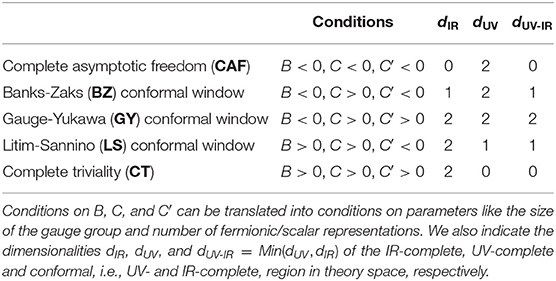
Table 1. Different perturbative Renormalization Group phases for simple gauge-Yukawa theories.
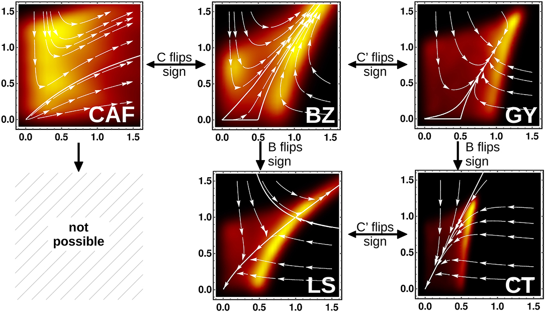
Figure 1. Possible RG structures, cf. [73] (see main text for further discussion), of simple gauge Yukawa-theories, depending on the signs of one- and two-loop coefficients B, C, and C′ of the gauge coupling β-function, cf. Equation (4) and in turn on the gauge group and matter content of the theory. The x-axis (y-axis) shows the gauge coupling αg (Yukawa coupling αy). Thick white lines indicate the boundary surface of the UV-complete, IR-complete, or conformal regions in theory space. White flow lines (arrows) point toward the IR. The heat maps in the background indicate how a set of random EFTs, uniformly distributed over the full depicted range of couplings, is focused toward the boundary surface. Lighter areas indicate a high density of theories one order of magnitude below the cutoff scale. The explicit β-function coefficients, cf. Equation (4), required to obtain the plots have been chosen as: CAF: B = C = C′ = E = F/2 = 1/10; BZ: 2B = −C = 2C′ = 2E = F = 1; GY: 2B = −C = −2C′ = 2E = 2F = 1; LS: −2B = −C = 2C′ = 2E = 2F = 1; CT: −2B = −C = −2C′ = 2E = 2F = 1.
Preceding the EFT discussion of these phases, it is important to distinguish the following terminology. A set of gauge-Yukawa theories is determined by its gauge group and matter content, parameterized, for instance, by the number of fermionic representations NF. To agree with previous literature [112], we refer to the possible values of NF which realize certain gauge-Yukawa phases as “windows.” This is distinct from a particular realization within a set of gauge-Yukawa theories. The latter is further parameterized by coupling values, i.e., by a choice of RG trajectory. When referring to possible values of the couplings, we talk about “regions.” In particular, we say that the set of all UV-complete trajectories makes up the UV-complete region, the set of all IR-complete trajectories makes up the IR-complete region, and the set of all UV- and IR-complete trajectories makes up the “conformal” region. Crucially, the terminology “conformal window” and “conformal region” are to be distinguished.
2.1. Complete Asymptotic Freedom (CAF)
For antiscreening B > 0 as well as C > 0, the only physical fixed point is the Gaußian one, cf. left-hand upper panel in Figure 1. The former is completely asymptotically free when approached from below the Yukawa nullcline, i.e., whenever Y < Y*(αg). This case also encompasses asymptotic freedom of Yang-Mills theory without Yukawa couplings, cf. the RG flow along the x-axis in the left-hand upper panel of Figure 1. The UV-complete region is 2-dimensional and extends to infinite coupling values (or more accurately beyond perturbative control) although it is partially bound by the Yukawa-nullcline (white line). This boundary surface inherits the IR-attractive property of the free fixed point along the Yukawa direction (y-axis) and is hence IR-attractive from above, i.e., for Y > Y*. This entails that generic UV-incomplete EFTs will be attracted to the boundary. The IR-complete (and thus also the conformal) region is reduced to the trivial theory. All other theories eventually escape perturbative control toward the IR.
2.2. Banks-Zaks (BZ) Conformal Window
Scalar, as well as fermionic matter, adds screening fluctuations and modifies the running of non-Abelian gauge couplings. This can flip the signs of C, C′, and B. Independent of the specific matter representation, the sign of C is always flipped first and the theory (with vanishing Yukawa couplings) enters the so-called conformal window [112], cf. upper panel in the middle of Figure 1. As C flips sign (but before C′ or B do so), the Banks-Zaks fixed point becomes physical. For vanishing Yukawa coupling and 0 < αg < αg*, BZ, the theory is now both UV- and IR-complete. In fact, since the IR-complete and thus the conformal region is still only one-dimensional, the RG-scale can be mapped directly to a unique gauge-coupling value. Put differently, there only exists a single conformal theory. The gauge-Yukawa fixed point is still not physical and thus every theory with non-vanishing Yukawa coupling will eventually diverge in the IR. This is a consequence of the Banks-Zaks fixed point being IR-attractive in the direction of the gauge coupling but IR-repulsive in the direction of the Yukawa coupling. To distinguish this situation, we refer to this as the “BZ conformal window.” However, the UV-complete region is still two-dimensional. Its boundary inherits the partial IR-attractive nature of the two fixed points. (The free fixed point is IR-attractive in the Yukawa-coupling direction and the Banks-Zaks fixed point is IR-attractive along the gauge-coupling direction). The corresponding sections of the boundary surface act as an IR-attractor, in particular for EFTs outside of the UV-complete region. We emphasize that it is the boundary and not a single fixed point which is IR-attractive.
Adding further matter representations can flip the sign of C′ or B first. Therefore, there are now two distinct phases that can occur when further matter is added. Which of these is realized depends on the ratio of scalar and fermionic matter and on the set of possible Yukawa interactions.
2.3. Gauge-Yukawa (GY) Conformal Window
Whenever C′ turns negative before B does, the theory develops a fully IR-attractive gauge-Yukawa fixed point, cf. right-hand upper panel in Figure 1. As C′ is varied, the fixed point formally enters from infinity (or from outside the perturbative regime) along the direction in which the two nullclines of the BZ phase join. The gauge-Yukawa fixed point serves as an endpoint of the two nullclines and delimits the two-dimensional UV-complete region, which is now also IR-complete. As a consequence, there is now a two-dimensional region of distinct conformal theories. In correspondence to the “BZ conformal window,” we refer to this as the “gauge-Yukawa (GY) conformal window.” This case is particularly predictive. If realized only over a finite range of scales, e.g., due to the decoupling of massive modes, this realizes effective asymptotic safety. All EFTs are attracted first to the boundary of the “gauge-Yukawa conformal window” and eventually into the gauge-Yukawa fixed point.
2.4. Litim-Sannino (LS) Conformal Window
If, on the other hand, B turns negative before C′ does, a Litim-Sannino fixed point [22] becomes available, while the Banks-Zaks fixed point [112] disappears (formally it escapes the perturbative regime in direction of increasing gauge coupling) and the free fixed point becomes fully IR-attractive, cf. lower panel in the middle of Figure 1. It is now the IR-complete region which is two-dimensional. However, the UV-complete region and hence the set of conformal theories, is just one-dimensional. The latter is delimited by the free and the Litim-Sannino fixed point, while the former also extends beyond the Litim-Sannino fixed point and corresponds to its UV-critical hypersurface. Concerning generic EFTs, the conformal theory which splits the IR-complete region, i.e., the separatrix between the Litim-Sannino and the free fixed point, acts as an IR-attractor because it inherits this property from the shared IR-attractive direction of both its delimiting fixed points. The boundary of the IR-complete region, however, is not IR attractive since it inherits the IR-repulsive direction of the Litim-Sannino fixed point. Again, generic EFTs tend to cluster close to the UV-complete theories, i.e., exhibit effective asymptotic safety.
2.5. Complete Triviality (CT)
The final possibility occurs if all three signs are flipped, i.e., B < 0 and C < C′ < 0. Since all contributions have now turned screening, the theory remains only with the free fixed point. The latter is now fully IR-attractive. This phase occurs for the perturbative range of any Abelian gauge group, cf. section 3.2. Formally, the UV-complete and conformal regions reduce to the trivial theory to which all EFTs are attracted. The IR-complete region now covers all of the theory space. The triviality problem can therefore be seen as a consequence of “effective asymptotic freedom.”
This concludes the review of all possible fixed-point structures [73] which can occur due to different cancelations at NLO in simple gauge-Yukawa theories. One can schematically think of semi-simple cases, such as the SM, as the higher-dimensional combinations of these phases, cf. [34] for an explicit discussion. In the following, we will always check whether potential fixed points persist at NNLO. We present our formal definition of perturbativity in section 4. Before doing so, we provide insight into the single gauge groups of the SM which is sufficient to qualitatively understand the available fixed points that we identify in the coupled system in section 6. In all phases, some form of IR-attractor dominates the RG flow.
3. Available Phases for the Simple Standard-Model Subgroups
Following [22], we remain focused on a simple gauge group with NF copies of a single type of fermionic representation RF and uncharged scalars to allow for Yukawa couplings, cf. Appendix A or [22] for the explicit Lagrangian. In this case, the Yukawa-coupling matrices E(Y) and F(Y) in Equation (2) reduce to scalar coefficients E and F of a single Yukawa coupling y for which we introduce . The NLO coefficients that determine the interacting fixed-points, cf. Equations (5) and (6) and the resulting RG-structure are given by, cf. [73],
Here, and dadj refer to the second Casimir and the dimension of the adjoint representation, respectively. Similarly, and denote the same for the fermionic representation5.
Naively, there are two ways to achieve perturbativity of the possible fixed points and , i.e., either by (i) making B small, or by (ii) making C or C′ large. It is typically not possible to achieve the latter (as a function of NC and NF for instance) without invalidating perturbation theory at higher orders. The subsequent discussion of the U(1) in section 3.2 will serve as an explicit example. On the contrary, non-Abelian gauge groups can allow for perturbatively small B without invalidating perturbation theory [22]. A dedicated 3-loop analysis of a simple SU(N) gauge group with fermions in the fundamental representation [38] provides strong indications that perturbative yet interacting gauge-Yukawa fixed points are only possible for NC ⩾ 5. However, this does not necessarily imply that the same conclusions hold for arbitrary representations. For extensions of the SM, this has been tested by an explicit grid search for a single type of BSM representation in [40]. Before extending such a grid search to multiple different types of BSM representation, we discuss each of the simple SM subgroups on its own. This provides a good intuition of why certain phases, cf. Figure 1, are possible and others are not.
3.1. The Non-Abelian Subgroups of the SM
Which of the gauge-Yukawa phases is accessible in perturbation theory depends on the sign of C′ in the region close to a sign-change of B, cf. Figure 1. Note that the sign of C is always fixed close to a sign change of B, cf. [73]. The sign of C′, in turn, depends on the specific gauge group and matter representations. In particular, additional fermionic representations without (or with negligibly small) Yukawa couplings result in additional screening contributions to B and C, while they do not contribute to (C′ − C) since they do not participate in Yukawa interactions. Hence, charged fermions without Yukawa couplings will influence which phases are available.
The latter also occurs in the SM where there are 32 light Weyl degrees of freedom with negligibly small Yukawa couplings6. We explicitly visualize their significance for the existence of gauge-Yukawa fixed points in the case of SU(2) and SU(3) in Figure 2. Without the SM fermions, there exist BSM representations [such as the d2 = 3 dimensional for SU(2) and the d3 = 8 dimensional for SU(3)] for which, with growing number NF of BSM fermions, B changes sign before C′ does. As a function of NF one moves from complete asymptotic freedom to the Banks-Zaks phase and into the Litim-Sannino phase, i.e., through the chain CAF → BZ → LS, cf. first and third panel in Figure 2. In particular, one enters the LS phase via a sign change in B, i.e., in the region in which the interacting fixed points can be perturbatively controlled. Inclusion of the SM fermions prohibits the realization of this chain, i.e., there is no possible BSM representation for which B changes sign before C′ does. When adding additional BSM representations one therefore always follows a different chain with growing NF: starting from complete asymptotic freedom and moving through the Banks-Zaks phase, one instead enters the gauge-Yukawa and ends up in the completely trivial phase, i.e., this realizes the chain CAF → BZ → GY → CT. For most BSM representations which can be added to the SM case, the BZ and GY phase only occur at non-integer values of NF such that this formal chain is effectively reduced to CAF → GY → CT or CAF → CT, cf. Figure 2. Formally, this chain can be prolonged and the LS phase can still be entered from the CT phase, cf. upper-right area of the second panel in Figure 2. The minimal (but quite large) number of BSM fermions identified in [37] realizes this formal window of the LS phase. While this can occur at small values of the couplings if C′ ≫ B ≫ 1, the latter invalidates perturbation theory and such fixed points are lost at NNLO, cf. also [40].
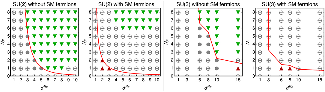
Figure 2. Different phases, i.e., LS (▾), GY (▴), BZ (●), CAF (⊕), and CT (⊖), of SU(2) and SU(3) gauge groups depending on the number NF and dimension (cf. Equations 30–31) of the included BSM representations and on whether the SM matter fields are included or not. The thick red curve highlights where the 1-loop contribution vanishes, i.e., B = 0. Interacting fixed points can only be controlled perturbatively if they lie in the vicinity of this line. The LS phase recedes from the perturbatively accessible region whenever the SM fields, i.e., charged matter without or with neglibily small, Yukawa couplings are included.
Regarding extensions of the SM, we can conclude that the SM fermions with negligibly small Yukawa couplings prohibit from entering the LS phase, i.e., no perturbatively controlled, interacting fixed points with UV-attractive directions are possible. On the contrary, fully IR-attractive interacting gauge-Yukawa fixed points in the GY phase remain possible for special dimension and number of BSM representations, cf. red upward triangles in Figure 2. As we shall see in section 6, both conclusions persist for the full SM gauge group. The GY phase realizes effective asymptotic safety if the theory space is extended to include mass terms or scalar vacuum expectation values. In this case, the theory departs from (close to) the otherwise fully IR-attractive fixed point at RG scales below this mass threshold.
3.2. Persistence of Abelian Triviality
Despite the complete asymptotic freedom of both non-Abelian subgroups, the SM is not UV-complete, i.e., it eventually breaks down at a transplanckian but finite energy scale. Due to the lack of antiscreening self-interactions in the U(1) gauge group, matter fluctuations dominate and screen the associated Abelian gauge coupling. At ~ 1041 GeV, the latter grows beyond perturbative control and eventually results in a perturbative divergence—the Landau pole [113]. Beyond perturbation theory, the U(1) triviality problem has been confirmed by different non-perturbative methods [114–116], but so far only in the absence of Yukawa couplings.
Indeed, the presence of a Yukawa coupling formally places an Abelian gauge group in the Litim-Sannino phase, cf. section 2. Unfortunately, the corresponding interacting pseudo-fixed-point cannot occur within the perturbatively controlled regime. Since we found no explicit discussion of the latter statement in the literature, we will provide it in the following.
In principle, every U(1) gauge group with NF fermions of charge Y and associated scalars to facilitate Yukawa couplings is in the LS phase which would indicate the presence of an interacting UV fixed point for the gauge coupling at
The explicit NLO and NNLO β-functions are presented in Appendix C. It would seem as if this fixed point becomes more perturbative for large Y2 and large NF but this ignores the accompanying growth of higher-loop contributions and the resulting breakdown of perturbation theory. To properly analyze the above fixed point, one has to introduce a t'Hooft-like rescaling of the couplings. More specifically, one has to rescale the couplings αg and αy such that all higher-loop contributions either vanish or at least converge to finite values at large NF and large Y2. In the present case, the minimal rescaling that suppresses all higher-loop contributions with growing NF and Y2 is given by
The correspondingly rescaled β-functions reveal that (in contrast to the non-Abelian case in [22]) only the trivial fixed point persists in the perturbative large-charge–large-NF limit. We have explicitly confirmed that for any combination of integer NF ⩾ 0 and arbitrary Y2, the absolute value of the NNLO contributions is larger than that of the NLO contributions when evaluated at the fiducial fixed point in Equation (10)—a clear sign that perturbation theory is not valid anymore.
The physical mechanism through which the Litim-Sannino fixed point arises, i.e., the balance of screening contributions from fermionic fluctuations against antiscreening contributions from Yukawa couplings, is present nevertheless. Thus, it might be worthwhile to conduct a non-perturbative analysis of this fixed-point mechanism in Abelian theories with Yukawa couplings in the future. However, for the present perturbative analysis, we conclude that the Abelian gauge group of the SM will always remain trivial.
4. A Quantitative Measure of Predictivity
For a given gauge-Yukawa theory with fixed gauge group and matter content, we define the perturbative range of coupling values αi by the condition that all NNLO contributions remain smaller than the respective NLO contributions, i.e.,
The factor is included such as to avoid the regime of novel fiducial fixed points arising at NNLO. Another reason for the inclusion of this factor is the U(1) Landau pole, as will become clear below. This perturbativity condition is rather non-conservative, meaning that perturbation theory may break down earlier. The resulting set of perturbative EFTs encloses a finite volume in the (truncated) theory space of all couplings7. More explicitly, we use the volume of the convex hull obtained from a Delauney-triangulation of a large enough random set of points in theory space which fulfill the perturbativity criterion8. We ensure convergence of this discrete volume measure by averaging over several individual random sets of perturbative EFTs and making sure that the statistical error is subleading.
The theory-space volume depends on the definition of couplings: for instance, a simple rescaling of couplings will also rescale . It is thus certainly a scheme-dependent statement. However, ratios of such volumes at different scales measure something like an overall critical exponent and should, therefore, capture scheme-independent effects9. Taking such ratios allows us to define a quantitative measure of predictivity. The theory-space volume can be evolved by following the RG flow to the IR. Given the initial volume Λ at the cutoff scale Λ, and its evolution following the RG flow, i.e., k, at RG scale k, we define predictivity (k) by
We call EFTs predictive (non-predictive), whenever their theory-space volume decreases (increases) along the flow. Non-predictive EFTs tend to formally result in (k) → ∞ at finite k < Λ which signals that they have diverged beyond perturbative control. In the predictive case, however, (k) provides a quantitative measure of how predictive the EFT is. We caution that, at present, we are not able to provide proof that the predictivity measure constitutes a scheme-independent statement. We hope to sharpen the scheme-independence of this definition in future work.
It will also prove useful to exclude specific couplings, e.g., the measured SM couplings, from the predictivity measure and instead match them to their experimentally known values at a specified low-energy scale, e.g., at Λew < Λ. The resulting can measure partial predictivity, even if the overall EFT is classified as non-predictive.
Both, the predictivity and the partial predictivity measure do not necessarily rely on perturbation theory and can be applied to (sufficiently converged) non-perturbative truncations of theory space as well. However, they do require to define an initial volume in theory space in which the present truncation is sufficiently converged, i.e., a non-perturbative analog of Equation (12). Whenever such an initial volume in theory space can be defined, its evolution under the RG flow allows us to quantify the predictivity of effective asymptotic safety via the measure in Equation (13). In particular, this applies to truncations of the Reuter universality class [66], see [67–69] for introductory texts and [65, 70–72] for previous discussions in the effective asymptotic safety context. We leave such an analysis for future work.
To exemplify the above definitions, we will discuss the heavy gauge-Yukawa sector of the SM in section 5 before adding new matter degrees of freedom in section 6.
5. The Heavy-Top Limit of the Standard Model
We focus on the heavy gauge-Yukawa sector of the SM, i.e., on the three gauge couplings α1,2,3 and the top-Yukawa coupling αt. It is a very good approximation to assume all other fermions as being massless, i.e., to set their Yukawa couplings to zero. Similarly, we neglect contributions from the quartic coupling λ4 which is also negligible with regards to the gauge-Yukawa sector, as long as all couplings remain within the perturbative regime because it only arises at 2-loop and 3-loop order for Yukawa and gauge couplings, respectively. Supplementary conditions implied by stability conditions of the Higgs potential [24, 38] are deferred to future studies.
5.1. Partial Predictivity Within the Standard Model
The heavy SM is non-predictive, i.e., (k) quickly diverges below the cutoff scale. This is a result of the antiscreening nature of the non-Abelian gauge couplings realizing the CAF phase, cf. section 2 in the SM. Coupling values at the cutoff scale that lie close to the edge of the perturbative regime will quickly be driven to values beyond perturbative control toward the IR.
On the other hand, if one excludes the non-Abelian gauge couplings from the predictivity measure and instead fixes them to their known experimental values at the electroweak scale, the SM is partially predictive in the remaining theory space. This is a consequence of the screening nature of both the top-Yukawa and the U(1) gauge coupling. When excluding also the U(1) gauge coupling from the predictivity measure, the resulting partial predictivity reflects the pre-Tevatron situation in which all the gauge couplings had already been experimentally measured, while the top-Yukawa coupling αt remained unknown. Figure 3 shows the evolution of along the RG flow. In this simple one-dimensional slice of theory space, the predictivity measure simply amounts to the normalized evolution of the full perturbative range of top-Yukawa values below ΛPlanck. Hence, enforcing a perturbative origin at ΛPlanck bounds the top quark to be lighter than Mt ≲ 210GeV. The underlying reason is the associated partial IR fixed point for Yukawa couplings in gauge-Yukawa theories previously uncovered in [109–111], cf. also Equation (3).
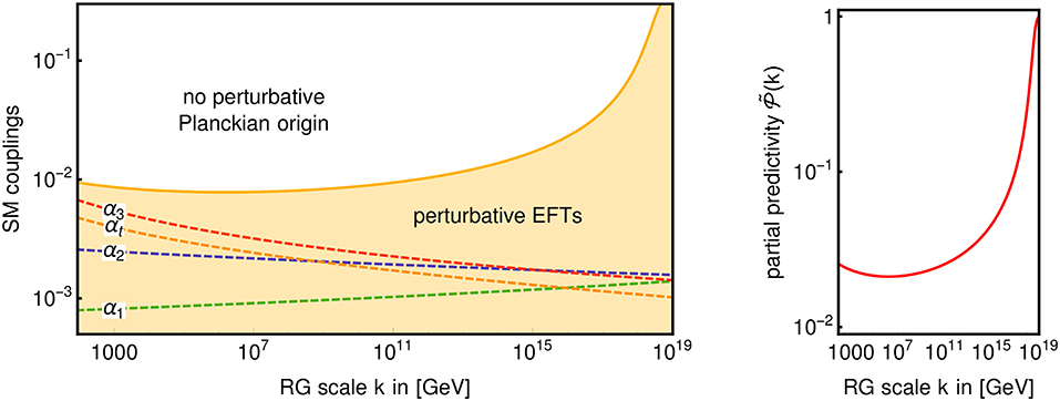
Figure 3. (Left) RG flow of the SM gauge-Yukawa theory. The shaded region indicates values for αt which can originate from a perturbative EFT at the cutoff scale ΛPlanck. The focusing of this region toward the lower scales exemplifies the partial predictive power of the SM as an EFT. The dashed trajectories indicate the RG flow of α3, α2, α1, and αt, matching observed values at the electroweak scale. (Right) Evolution of the partial predictivity measure with the RG flow.
5.2. The Landau Pole Remains Transplanckian
As discussed in section 3.2, the triviality of the U(1) hypercharge cannot be cured within perturbation theory. On the other hand, the associated Landau pole remains above the Planck scale as long as the other SM couplings remain within the perturbative regime (and no BSM representations with hypercharges are added).
Even in the absence of any new states with hypercharge, NLO and NNLO contributions from the non-Abelian gauge and top-Yukawa couplings in a modified BSM RG flow can potentially further screen the U(1) gauge coupling and therefore result in a lowered Landau pole, cf. also [37]. However, for any perturbative extension of the SM that still matches the measured electroweak-scale value for α1, the Landau pole remains at transplanckian energies. One can numerically determine that α3 ≲ 0.15, α2 ≲ 0.09, and αt ≲ 0.53 is required to conform to the perturbativity criterion in Equation (12), i.e., to . These maximal values have been determined by a grid search at random α1. We then fix the non-Abelian gauge couplings and the top Yukawa coupling to these maximal values. By definition, any RG flow within the perturbative regime cannot outgrow these values. Numerical integration of the resulting RG flow of the U(1) coupling shows that the U(1)-Landau pole remains safely beyond the Planck scale.
The left panel in Figure 4 shows the RG-flow of the Abelian gauge coupling matching to the observed electroweak-scale value for a random set of fixed values of the other heavy-SM couplings satisfying the perturbativity criterion. Subplanckian Landau poles are not present. Loosening the perturbativity criterion in Equation (12) to |β(NNLO)| < |β(NLO)| allows for rare cases at the edge of the redefined perturbative regime for which the Landau pole is shifted slightly below the Planck scale, cf. right panel in Figure 4. In any case, all the perturbative BSM fixed points discussed in section 6 are much more perturbative than any of the above bounds.
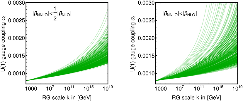
Figure 4. RG-flow of the U(1) gauge coupling matched to the observed electroweak value for arbitrary non-Abelian gauge and top-Yukawa couplings within the perturbative regime. (Left) perturbativity defined by , cf. Equation (12). (Right) Perturbativity defined by .
We conclude that the persistence of a U(1)-Landau pole—at least in any of the subsequently important BSM scenarios in which the BSM representations do not carry hypercharge—is no meaningful criterion in the search for physically interesting fixed points in the framework of perturbative EFTs below the Planck scale. Instead, one should merely verify that the Landau pole remains transplanckian. In this aspect, we advocate a different point of view, than, e.g., [40].
6. New Matter Degrees of Freedom
In the following, we allow for additional fermionic matter in arbitrary representations (as well as for the associated uncharged scalars to facilitate Yukawa couplings). We have seen that, within perturbation theory, any U(1) factor will remain trivial. Therefore, we do not attempt to modify the RG flow of the U(1) gauge coupling and thus only add BSM fermions which are uncharged under the U(1). We allow for an arbitrary number of different representations of BSM fermions, i.e., fermions in the -dimensional representation of SU(2) and SU(3), respectively. The Lagrangian (see Equation 25) and the β-functions for the three gauge couplings, the top-Yukawa coupling, as well as additional BSM Yukawa couplings, i.e., for
are generalized from [40] and collected in Appendix B. We emphasize that while the BSM scalars are uncharged, fluctuations of the charged SM Higgs scalar are always included.
With the intuition from the results in section 2 for simple non-Abelian gauge groups, we anticipate that, also in the semi-simple case, the non-Abelian subgroups cannot admit perturbatively controllable Litim-Sannino fixed points with an IR-repulsive (UV-attractive) direction. We confirm this expectation in the following explicit analysis. Fully IR-attractive gauge-Yukawa fixed points, on the other hand, can exist. From the viewpoint of effective asymptotic safety, these are the most predictive and in that sense most interesting fixed points, anyhow.
The larger the dimension of the BSM representations, the greater their screening effect on the 1-loop coefficient of the associated non-Abelian gauge coupling. Thus, there exists an upper dimension and beyond which even a single additional BSM representation will always push the associated non-Abelian SM gauge group into the completely trivial phase. Hence, the set of possible BSM representations for which perturbative non-vanishing gauge-Yukawa fixed points might exist is limited and easily tractable. With the help of computer algebra [117], we simply scan through all possibilities and identify those for which the NLO beta-functions exhibit a fixed point with
We subsequently test the perturbativity of each of the resulting fixed points by initializing a numerical root search in the NNLO beta-functions at the NLO fixed-point values. If the latter converges, we compare whether the signs of the critical exponents of the NLO and NNLO fixed points match. (If the root search does not converge, we discard the NLO fixed point). Thereby we can identify perturbative fixed points for which NNLO corrections are subleading10.
Irrespective of the specific representation and the number of copies , we find that a single type of BSM representation R1 is insufficient to generate a fixed point at which both α2* ≠ 0 and α3* ≠ 0. IR-attractive gauge-Yukawa fixed points at which only one of the non-Abelian gauge couplings is non-vanishing are available in perturbation theory and have been identified in [40].
Proceeding to two different types of representations, i.e., R1 and R2, we are able to identify a single combination of BSM representations for which a fixed point as in Equation (15) is possible, i.e.,
Having specified the above representations, the respective BSM Lagrangian follows from Equation (25 in Appendix B). For this specific combination of BSM representations, both non-Abelian gauge groups are in the GY phase. Hence, all possible combinations of gauge-Yukawa fixed points exist. In particular, this includes a fully IR-attractive fixed point at
The fixed point persists at NNLO order.
To summarize, we find that by adding suitable matter content to the SM, the non-Abelian gauge-Yukawa sector of the SM can transition from the CAF-phase to the GY-phase, and of course to the CT-phase. The explicit study supports that neither the BZ-phase nor the LS-phase is possible, cf. section 3. Within perturbation theory, the U(1) always remains in the CT-phase.
6.1. Predictivity Below the Planck Scale
For simple gauge-Yukawa theories in the CAF phase (BZ phase), the IR-complete region is reduced to the free theory (one-dimensional conformal window for vanishing Yukawa coupling), cf. Figure 1. Hence, these phases develop IR divergences for initial conditions that lie close to the edge of perturbativity at the cutoff scale. Put differently, they are non-predictive (as defined in section 4). On the contrary, the IR-complete region of theories in the GY or CT phase (and the LS) phase is two dimensional and covers all (or most) of the perturbative regime. Hence, these phases are predictive.
In Equation (16), we have identified a combination of BSM representations to push the non-Abelian SM subgroups into the predictive GY but not yet trivial phase. The two right-hand panels in Figure 5 depict the associated decreasing volume in theory space as a function of the RG-flow toward the IR in two slices of the overall 6-dimensional theory space. The left-hand panel shows the corresponding evolution of the predictivity measure (k). Specifying to , the theory-space volume is reduced by a factor of between ΛPlanck and ΛNP.
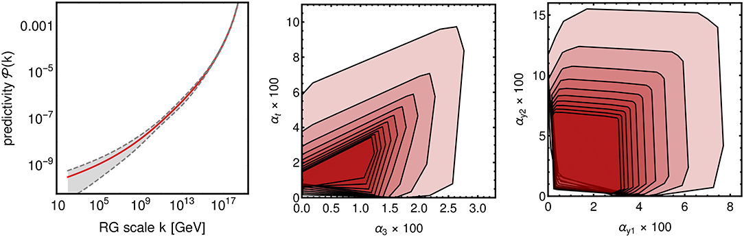
Figure 5. In the left panel we show the predictivity of the BSM model identified in Equation (16), averaged over 10 sets of perturbative but otherwise random initial EFTs. The gray-dashed region indicates the statistical error. The other two panels show projections of the evolving theory-space volume [onto the α3-αt-plane (middle) and onto the --plane (right)]. We plot its convex hull at each order of magnitude below ΛPlanck with increasingly darker-red shading toward the IR.
Despite fixed-point values that depart significantly, i.e., by several 100%, from the measured SM values, predictivity is insufficient to exclude the BSM extension from matching to the SM electroweak scale. Put differently, the observed SM-coupling values lie within the “conformal” region of UV- and IR-complete theories (apart from the non-vanishing value of the Abelian gauge coupling, cf. section 3.2).
6.2. Partial Predictivity Below the Planck Scale
A phenomenologically more relevant question is that of partial predictivity under the condition of matching all the observed SM couplings, i.e., α1, α2, α3, and αt, to their measured electroweak-scale values. The resulting partial predictivity for the BSM Yukawa couplings—especially in αy1—is quite strong. Figure 6 shows how the RG flow strongly focuses the BSM Yukawa couplings toward the IR, all the while enforcing that the SM couplings match to their electro-weak scale values. The full range of perturbative EFT values at ΛPlanck is mapped to values below the partial fixed point, i.e., αy1(k = Λew) ≲ 0.0165 and αy2(k = Λew) ≲ 0.0083. These values do not precisely match with the fixed-point values in Equation (17) because the SM couplings are matched to their electro-weak scale values, instead.
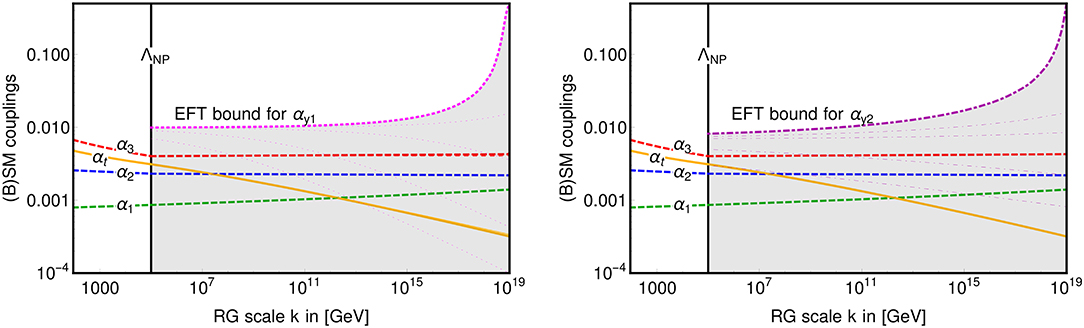
Figure 6. Partial predictivity for the BSM theory identified in Equation (16). The plots show RG trajectories that match the observed values of SM couplings in the heavy-top limit, i.e., α1, α2, α3 (dashed), and αt (continuous). At energies below (above) ΛNP, the BSM degrees of freedom decouple (are active). The BSM RG flow focuses arbitrary perturbative initial conditions for the BSM Yukawa couplings αy1 (left) and αy2 (right) at the Planck scale to the gray-shaded regions at lower scales. We also indicate (thin lines) several trajectories to exemplify the behavior of different RG trajectories within the conformal region.
In general, any RG trajectory for the BSM Yukawa couplings in the gray region of Figure 6 is possible. However, typical initial conditions, i.e., those which are not fine-tuned to values very close to zero, are all mapped to values very close to the partial fixed-point value, cf. thin lines in Figure 6. This is a result of the power-law scaling toward the interacting fixed point in Equation (17) (more specifically, toward its partial counterpart). Quantitatively, the RG flow maps initial conditions within the perturbative but “natural” range of coupling values at the Planck scale to a very narrow window at the electroweak scale, i.e., to . Assuming that the BSM Yukawa couplings should take such “natural,” i.e., (1), values at the Planck scale, therefore predicts . We caution that a correct matching to the SM values of αt requires the latter to have an “unnatural” Planck scale value ~10−5, thereby questioning the use of the above naturalness assumption. Similar arguments also apply to αy2, although partial predictivity is less pronounced, cf. Figure 6.
The above partial predictivity does not rely on the existence of a gauge-Yukawa fixed point like the one found in Equation (17). It is merely a consequence of the partial IR fixed-point for the BSM Yukawa couplings, cf. Equation (3). We list some explicit examples of BSM matter content to realize the CAF, GY, and CT phase (for both non-Abelian gauge groups) along with predictivity and partial predictivity in Table 2. It can be concluded that while only theories in the GY and the CT phase are predictive, partial predictivity persists in all models. In particular, the partial predictivity in the absence of a gauge-Yukawa fixed point can outgrow the partial predictivity in the presence of one.
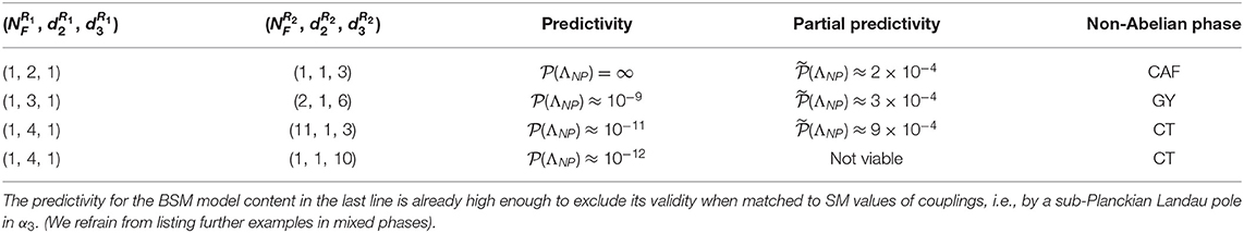
Table 2. Preditictivity (ΛNP) and partial predictivity at a new-physics scale for some selected BSM models in the three available phases characterized by their BSM matter content in the first two columns, see main text for further discussion.
7. Discussion
We have analyzed the fixed points of gauge-Yukawa theories and, in particular, the SM gauge group in the context of EFTs below the Planck scale. For the SM gauge groups, we have clarified why gauge-Yukawa fixed points with UV-attractive directions cannot occur within the perturbatively controlled regime. However, additional matter fields can result in a perturbative and fully IR-attractive gauge-Yukawa fixed point which realizes effective asymptotic safety. We have introduced a novel quantitative measure for the predictivity of general EFTs and have applied it to gauge-Yukawa BSM extensions. Concerning concrete BSM phenomenology, this allows us to make the following conclusions:
• The results highlight that the presence of an (Abelian) Landau pole, as long as it occurs at trans-Planckian scales, does not pose a strict no-go criterion in the search of perturbative interacting fixed points in non-gravitational and hence necessarily effective theories with a Planckian cutoff.
• We have identified a fully IR-attractive and (apart from the Abelian gauge coupling) fully interacting fixed point if suitable vector-like fermions without hypercharge, i.e., one SU(3) singlet in the three-dimensional representation of SU(2) and two SU(2) singlets in the six-dimensional representation of SU(3), are added to the SM, cf. Equations (16) and (25 in Appendix B) for the corresponding BSM Lagrangian. This particular theory is predictive along the RG flow toward the IR. We have quantified its predictive power and compared it to other BSM models without interacting fixed points. For all these models, partial predictivity restricts the range of coupling values of the BSM Yukawa couplings in dependence on the ratio between the BSM scale and the cutoff scale.
• In general, the predictive power of subplanckian effective asymptotic safety of gauge-Yukawa theories can be estimated by a simple argument: Let ϵ≪1 be the perturbative parameter. For simple gauge-Yukawa theories, ϵ ≲ 0.1 has been found in [22] as the indicated regime of perturbative control. Perturbative fixed points that come about by the balance of loop orders will necessarily result in critical exponents θ proportional to some power of ϵ, i.e., θ ≲ ϵ. Extrapolating the linearized regime around the fixed point, one therefore expects (α(ΛIR) − α*)/(α(ΛUV) − α*) = ϵlog(ΛIR/ΛUV) for the associated coupling α. For the phenomenologically important case of , predictivity is thus expected to be limited to shrinking the allowed region of all perturbative coupling values by one or two orders of magnitude. This simple argument also motivates that predictivity can be further increased (i) for non-perturbative fixed points—as e.g., tentatively suggested in a toy model in [118]—because θ need not be small and (ii) for potential fixed points including gravitational fluctuations, see e.g., [119–122] since ΛUV can be extended beyond the Planck scale.
More generally, the example of gauge-Yukawa theories suggests that the boundaries of all UV-complete and/or IR-complete theories constitute special hypersurfaces in the theory space. In particular, we have made the following observations.
• The boundary hypersurfaces separate theories on both sides. Whenever one is confident that such a boundary exists and one knows that experimentally observed values lie either inside or outside, one can exclude that the observed IR physics originates from UV physics on the other side of the boundary.
• Moreover, the boundary surfaces can inherit the IR-attractive properties of their delimiting fixed point. In such cases, generic EFTs at the cutoff scale—both UV complete and not UV complete—will converge to realize coupling values closer to the boundary surface toward the IR. This is a first step to generalize the local notion of fixed points to global IR-attractors in theory space.
These two points highlight that knowledge about such boundary surfaces can be of great value whenever one tries to relate theories at different scales. Of course, having all the information to exactly reconstruct the boundary surface amounts to knowing about all RG flows in its vicinity. One might, therefore, object that with this information one could directly evolve a theory between different scales and obtain its counterpart at other scales. However, this is true only if one knows about all the coupling values at a given scale which is typically not the case in the search for new physics. The constraints on BSM Yukawa couplings, that partial predictivity and perturbativity up to the Planck scale entail, provide for an example to emphasize this more general point.
Data Availability Statement
The raw data supporting the conclusions of this article will be made available by the authors, without undue reservation.
Author Contributions
The author confirms being the sole contributor of this work and has approved it for publication.
Funding
This manuscript was supported by the Royal Society International Newton Fellowship NIF\R1\191008. The author also acknowledges open-access funding by the Imperial Open Access Fund.
Conflict of Interest
The author declares that the research was conducted in the absence of any commercial or financial relationships that could be construed as a potential conflict of interest.
Acknowledgments
The author is grateful to A. Eichhorn for many valuable discussions and comments on the manuscript as well as to C. Nieto for valuable discussion on [40].
Supplementary Material
The Supplementary Material for this article can be found online at: https://www.frontiersin.org/articles/10.3389/fphy.2020.00341/full#supplementary-material
Footnotes
1. ^This assumption can be circumvented by very weakly coupled particles, in which case the new-physics scale may lie below the electroweak scale. We will not discuss these cases here.
2. ^We caution that these observations require a truncation of the perturbative series or any other expansion which is sufficiently converged to have revealed all physical fixed points. Otherwise, the statement still applies to the truncated RG flow but might lose its phenomenological significance.
3. ^Given this setup, we are only able to make statements about those non-vanishing fixed points that potentially arise from a balance between leading order (LO) and NLO contributions. In principle, there could be further fixed points for which NNLO (or even higher) loop orders are required. However, one should then always be careful to test their nature by confirming that (at least) they persist upon inclusion of the subsequent higher-loop order. Since 3NLO contributions are not available at present, such an analysis cannot reliably be made.
4. ^We have chosen the signs to reflect the antiscreening non-Abelian case without matter content. Note that this choice agrees with [112] but differs from [22].
5. ^Either of the latter group-theoretic invariants can be traded for the Dynkin index
but note that the latter is defined only up to a constant and varying conventions are used in the literature. Here, we use the dimension and the second Casimir.
6. ^This counting excludes the top quark since its Yukawa coupling is not negligibly small. It also excludes potential right-handed neutrinos which are SM singlets anyway.
7. ^Since we work in the perturbative regime, all higher-order couplings will necessarily remain irrelevant. Hence, the UV-complete region does not extend in any of these directions and its volume, if finite in truncated theory space, remains finite in full theory space. Technically, this is not necessarily true for the overall EFT volume in the theory-space volume which permits an extension in any higher-order direction of the full theory space. We restrict to truncated theory space in the following.
8. ^One can easily see that the convex hull is not always a good approximation to the theory-space volume enclosed by the separatrices between fixed points, cf. upper right-hand panel in Figure 1. However, it is (to our knowledge) the only mathematically well-defined discrete notion of such a volume. It certainly suffices to quantify the statements of this study.
9. ^In case of a single fixed point and a purely linear flow, the ratio of theory-space volumes is indeed directly related to the critical exponents.
10. ^One might be able to construct more elaborate search algorithms and thereby potentially identify additional gauge-Yukawa BSM theories with perturbatively controlled interacting fixed points and we do not claim completeness.
References
1. Brivio I, Trott M. The standard model as an effective field theory. Phys Rept. (2019) 793:1–98. doi: 10.1016/j.physrep.2018.11.002
2. Donoghue JF. General relativity as an effective field theory: the leading quantum corrections. Phys Rev D. (1994) 50:3874–88. doi: 10.1103/PhysRevD.50.3874
3. Gross DJ, Wilczek F. Ultraviolet behavior of nonabelian gauge theories. Phys Rev Lett. (1973) 30:1343–6. doi: 10.1103/PhysRevLett.30.1343
4. Politzer HD. Reliable perturbative results for strong interactions? Phys Rev Lett. (1973) 30:1346–9. doi: 10.1103/PhysRevLett.30.1346
5. Cheng TP, Eichten E, Li LF. Higgs phenomena in asymptotically free gauge theories. Phys Rev D. (1974) 9:2259. doi: 10.1103/PhysRevD.9.2259
6. Kalashnikov OK. Asymptotically free SU(2) x SU(2) x SU(4) model of unified interaction. Phys Lett. (1977) 72B:65–9. doi: 10.1016/0370-2693(77)90064-8
7. Oehme R, Zimmermann W. Relation between effective couplings for asymptotically free models. Commun Math Phys. (1985) 97:569. doi: 10.1007/BF01221218
8. Kubo J, Sibold K, Zimmermann W. Higgs and top mass from reduction of couplings. Nucl Phys. (1985) B259:331–50. doi: 10.1016/0550-3213(85)90639-X
9. Kubo J, Sibold K, Zimmermann W. New results in the reduction of the standard model. Phys Lett B. (1989) 220:185–90. doi: 10.1016/0370-2693(89)90034-8
10. Zimmermann W. Scheme independence of the reduction principle and asymptotic freedom in several couplings. Commun Math Phys. (2001) 219:221–45. doi: 10.1007/s002200100396
11. Giudice GF, Isidori G, Salvio A, Strumia A. Softened gravity and the extension of the standard model up to infinite energy. J High Energy Phys. (2015) 02:137. doi: 10.1007/JHEP02(2015)137
12. Holdom B, Ren J, Zhang C. Stable asymptotically free extensions (SAFEs) of the standard model. J High Energy Phys. (2015) 03:028. doi: 10.1007/JHEP03(2015)028
13. Pelaggi GM, Strumia A, Vignali S. Totally asymptotically free trinification. J High Energy Phys. (2015) 08:130. doi: 10.1007/JHEP08(2015)130
14. Gies H, Zambelli L. Asymptotically free scaling solutions in non-Abelian Higgs models. Phys Rev D. (2015) 92:025016. doi: 10.1103/PhysRevD.92.025016
15. Pica C, Ryttov TA, Sannino F. Conformal phase diagram of complete asymptotically free theories. Phys Rev D. (2017) 96:074015. doi: 10.1103/PhysRevD.96.074015
16. Gies H, Zambelli L. Non-Abelian Higgs models: paving the way for asymptotic freedom. Phys Rev D. (2017) 96:025003. doi: 10.1103/PhysRevD.96.025003
17. Einhorn MB, Jones DRT. Asymptotic freedom in certain SO(N) and SU(N) models. Phys Rev D. (2017) 96:055035. doi: 10.1103/PhysRevD.96.055035
18. Hansen FF, Janowski T, Langãçble K, Mann RB, Sannino F, Steele TG, et al. Phase structure of complete asymptotically free SU(Nc) theories with quarks and scalar quarks. Phys Rev D. (2018) 97:065014. doi: 10.1103/PhysRevD.97.065014
19. Badziak M, Harigaya K. Asymptotically free natural supersymmetric twin higgs model. Phys Rev Lett. (2018) 120:211803. doi: 10.1103/PhysRevLett.120.211803
20. Gies H, Sondenheimer R, Ugolotti A, Zambelli L. Asymptotic freedom in ℤ2 -Yukawa-QCD models. Eur Phys J C. (2019) 79:101. doi: 10.1140/epjc/s10052-019-6604-z
21. Gies H, Sondenheimer R, Ugolotti A, Zambelli L. Scheme dependence of asymptotically free solutions. Eur Phys J C. (2019) 79:463. doi: 10.1140/epjc/s10052-019-6956-4
22. Litim DF, Sannino F. Asymptotic safety guaranteed. J High Energy Phys. (2014) 12:178. doi: 10.1007/JHEP12(2014)178
23. Sannino F, Shoemaker IM. Asymptotically safe dark matter. Phys Rev D. (2015) 92:043518. doi: 10.1103/PhysRevD.92.043518
24. Litim DF, Mojaza M, Sannino F. Vacuum stability of asymptotically safe gauge-Yukawa theories. J High Energy Phys. (2016) 01:081. doi: 10.1007/JHEP01(2016)081
25. Nielsen NG, Sannino F, Svendsen O. Inflation from asymptotically safe theories. Phys Rev D. (2015) 91:103521. doi: 10.1103/PhysRevD.91.103521
26. Rischke DH, Sannino F. Thermodynamics of asymptotically safe theories. Phys Rev D. (2015) 92:065014. doi: 10.1103/PhysRevD.92.065014
27. Intriligator K, Sannino F. Supersymmetric asymptotic safety is not guaranteed. J High Energy Phys. (2015) 11:023. doi: 10.1007/JHEP11(2015)023
28. Esbensen JK, Ryttov TA, Sannino F. Quantum critical behavior of semisimple gauge theories. Phys Rev D. (2016) 93:045009. doi: 10.1103/PhysRevD.93.045009
29. Mølgaard E, Sannino F. Asymptotically safe and free chiral theories with and without scalars. Phys Rev D. (2017) 96:056004. doi: 10.1103/PhysRevD.96.056004
30. Bajc B, Sannino F. Asymptotically safe grand unification. J High Energy Phys. (2016) 12:141. doi: 10.1007/JHEP12(2016)141
31. Pelaggi GM, Sannino F, Strumia A, Vigiani E. Naturalness of asymptotically safe Higgs. Front Phys. (2017) 5:49. doi: 10.3389/fphy.2017.00049
32. Abel S, Sannino F. Radiative symmetry breaking from interacting UV fixed points. Phys Rev D. (2017) 96:056028. doi: 10.1103/PhysRevD.96.056028
33. Christiansen N, Eichhorn A, Held A. Is scale-invariance in gauge-Yukawa systems compatible with the graviton? Phys Rev D. (2017) 96:084021. doi: 10.1103/PhysRevD.96.084021
34. Bond AD, Litim DF. More asymptotic safety guaranteed. Phys Rev D. (2018) 97:085008. doi: 10.1103/PhysRevD.97.085008
35. Abel S, Sannino F. Framework for an asymptotically safe Standard Model via dynamical breaking. Phys Rev D. (2017) 96:055021. doi: 10.1103/PhysRevD.96.055021
36. Bond AD, Litim DF. Asymptotic safety guaranteed in supersymmetry. Phys Rev Lett. (2017) 119:211601. doi: 10.1103/PhysRevLett.119.211601
37. Bond AD, Hiller G, Kowalska K, Litim DF. Directions for model building from asymptotic safety. J High Energy Phys. (2017) 08:004. doi: 10.1007/JHEP08(2017)004
38. Bond AD, Litim DF, Medina Vazquez G, Steudtner T. UV conformal window for asymptotic safety. Phys Rev D. (2018) 97:036019. doi: 10.1103/PhysRevD.97.036019
39. Bond AD, Litim DF. Price of asymptotic safety. Phys Rev Lett. (2019) 122:211601. doi: 10.1103/PhysRevLett.122.211601
40. Barducci D, Fabbrichesi M, Nieto CM, Percacci R, Skrinjar V. In search of a UV completion of the standard model–378,000 models that don't work. J High Energy Phys. (2018) 11:057. doi: 10.1007/JHEP11(2018)057
41. Hiller G, Hormigos-Feliu C, Litim DF, Steudtner T. Anomalous magnetic moments from asymptotic safety. arXiv[Preprint].arXiv:1910.14062 (2019).
42. Bond AD, Litim DF, Steudtner T. Asymptotic safety with Majorana fermions and new large N equivalences. Phys Rev D. (2020) 101:045006. doi: 10.1103/PhysRevD.101.045006
43. Hiller G, Hormigos-Feliu C, Litim DF, Steudtner T. Asymptotically safe extensions of the Standard Model with flavour phenomenology. In: 54th Rencontres de Moriond on Electroweak Interactions and Unified Theories (Moriond EW 2019). La Thuile (2019).
44. Mann R, Meffe J, Sannino F, Steele T, Wang ZW, Zhang C. Asymptotically safe standard model via vector-like fermions. Phys Rev Lett. (2017) 119:261802. doi: 10.1103/PhysRevLett.119.261802
45. Pelaggi GM, Plascencia AD, Salvio A, Sannino F, Smirnov J, Strumia A. Asymptotically safe standard model extensions? Phys Rev D. (2018) 97:095013. doi: 10.1103/PhysRevD.97.095013
46. Antipin O, Sannino F. Conformal window 2.0: the large Nf safe story. Phys Rev D. (2018) 97:116007. doi: 10.1103/PhysRevD.97.116007
47. Bajc B, Dondi NA, Sannino F. Safe SUSY. J High Energy Phys. (2018) 03:005. doi: 10.1007/JHEP03(2018)005
48. Sannino F, Skrinjar V. Instantons in asymptotically safe and free quantum field theories. Phys Rev D. (2019) 99:085010. doi: 10.1103/PhysRevD.99.085010
49. Molinaro E, Sannino F, Wang ZW. Asymptotically safe Pati-Salam theory. Phys Rev D. (2018) 98:115007. doi: 10.1103/PhysRevD.98.115007
50. Cacciapaglia G, Vatani S, Ma T, Wu Y. Towards a fundamental safe theory of composite Higgs and Dark Matter. arXiv[Preprint].arXiv:1812.04005 (2018).
51. Abel S, Mølgaard E, Sannino F. Complete asymptotically safe embedding of the standard model. Phys Rev D. (2019) 99:035030. doi: 10.1103/PhysRevD.99.035030
52. Wang ZW, Al Balushi A, Mann R, Jiang HM. Safe trinification. Phys Rev D. (2019) 99:115017. doi: 10.1103/PhysRevD.99.115017
53. Ryttov TA, Tuominen K. Safe glueballs and baryons. J High Energy Phys. (2019) 04:173. doi: 10.1007/JHEP04(2019)173
54. Orlando D, Reffert S, Sannino F. A safe CFT at large charge. J High Energy Phys. (2019) 08:164. doi: 10.1007/JHEP08(2019)164
55. Sannino F, Smirnov J, Wang ZW. Asymptotically safe clockwork mechanism. Phys Rev D. (2019) 100:075009. doi: 10.1103/PhysRevD.100.075009
56. Cai C, Zhang HH. Minimal asymptotically safe dark matter. Phys Lett B. (2019) 798:134947. doi: 10.1016/j.physletb.2019.134947
58. Bajc B, Lugo A, Sannino F. Safe Hologram. (2019). Available online at: https://arxiv.org/abs/1910.07354
59. Holdom B. Large N flavor beta-functions: a recap. Phys Lett B. (2011) 694:74–9. doi: 10.1016/j.physletb.2010.09.037
60. Alanne T, Blasi S, Dondi NA. Critical look at β -function singularities at large N. Phys Rev Lett. (2019) 123:131602. doi: 10.1103/PhysRevLett.123.131602
61. Sannino F, Wang ZW. Comment on “A critical look at β-function singularities at large N” by Alanne, Blasi and Dondi. (2019). Available online at: https://arxiv.org/abs/1909.08636
62. Cacciapaglia G, Pica C, Sannino F. Fundamental composite dynamics: a review. arXiv[Preprint].arXiv:2002.04914 (2020). doi: 10.1016/j.physrep.2020.07.002
63. Weinberg S. Ultraviolet divergences in quantum theories of gravitation. In: Hawking SW, Israel KW, editors. General Relativity: An Einstein Centenary Survey. (1980). p. 790–831.
65. Eichhorn A. An asymptotically safe guide to quantum gravity and matter. Front Astron Space Sci. (2019) 5:47. doi: 10.3389/fspas.2018.00047
66. Reuter M. Nonperturbative evolution equation for quantum gravity. Phys Rev D. (1998) 57:971–85. doi: 10.1103/PhysRevD.57.971
67. Percacci R. An Introduction to Covariant Quantum Gravity and Asymptotic Safety. Vol. 3 of 100 Years of General Relativity. World Scientific (2017). doi: 10.1142/10369
68. Reuter M, Saueressig F. Quantum Gravity and the Functional Renormalization Group. Cambridge: Cambridge University Press. (2019). Available online at: https://www.cambridge.org/academic/subjects/physics/theoretical-physics-and-mathematical-physics/quantum-gravity-and-functional-renormalization-group-road-towards-asymptotic-safety?format=HB&isbn=9781107107328
69. Eichhorn A. Asymptotically safe gravity. In: 57th International School of Subnuclear Physics: In Search for the Unexpected (ISSP 2019). Erice (2019).
70. Percacci R, Vacca GP. Asymptotic safety, emergence and minimal length. Class Quant Grav. (2010) 27:245026. doi: 10.1088/0264-9381/27/24/245026
71. Eichhorn A, Held A. Viability of quantum-gravity induced ultraviolet completions for matter. Phys Rev D. (2017) 96:086025. doi: 10.1103/PhysRevD.96.086025
72. de Alwis S, Eichhorn A, Held A, Pawlowski JM, Schiffer M, Versteegen F. Asymptotic safety, string theory and the weak gravity conjecture. Phys Lett B. (2019) 798:134991. doi: 10.1016/j.physletb.2019.134991
73. Bond AD, Litim DF. Theorems for asymptotic safety of gauge theories. Eur Phys J C. (2017) 77:429. doi: 10.1140/epjc/s10052-017-4976-5
74. Caswell WE. Asymptotic behavior of nonabelian gauge theories to two loop order. Phys Rev Lett. (1974) 33:244. doi: 10.1103/PhysRevLett.33.244
75. Jones DRT. Two loop diagrams in yang-mills theory. Nucl Phys B. (1974) 75:531. doi: 10.1016/0550-3213(74)90093-5
76. Tarasov OV, Vladimirov AA. Two loop renormalization of the yang-mills theory in an arbitrary gauge. Sov J Nucl Phys. (1977) 25:585.
77. Jones DRT. The two loop beta function for a G(1) x G(2) gauge theory. Phys Rev D. (1982) 25:581. doi: 10.1103/PhysRevD.25.581
78. Fischler M, Oliensis J. Two loop corrections to the evolution of the Higgs-Yukawa coupling constant. Phys Lett. (1982) 119B:385. doi: 10.1016/0370-2693(82)90695-5
79. Machacek ME, Vaughn MT. Two loop renormalization group equations in a general quantum field theory. 1. Wave function renormalization. Nucl Phys B. (1983) 222:83–103. doi: 10.1016/0550-3213(83)90610-7
80. Machacek ME, Vaughn MT. Two loop renormalization group equations in a general quantum field theory. 2. Yukawa couplings. Nucl Phys B. (1984) 236:221–32. doi: 10.1016/0550-3213(84)90533-9
81. Jack I, Osborn H. Background field calculations in curved space-time. 1. general formalism and application to scalar fields. Nucl Phys B. (1984) 234:331–64. doi: 10.1016/0550-3213(84)90067-1
82. Curtright T. Three loop charge renormalization effects due to quartic scalar selfinteractions. Phys Rev D. (1980) 21:1543. doi: 10.1103/PhysRevD.21.1543
83. Arason H, Castano DJ, Keszthelyi B, Mikaelian S, Piard EJ, Ramond P, et al. Renormalization group study of the standard model and its extensions. 1. The Standard model. Phys Rev D. (1992) 46:3945–65. doi: 10.1103/PhysRevD.46.3945
84. Pickering AGM, Gracey JA, Jones DRT. Three loop gauge beta function for the most general single gauge coupling theory. Phys Lett B. (2001) 510:347–54. doi: 10.1016/S0370-2693(01)00624-4
85. Luo Mx, Wang Hw, Xiao Y. Two loop renormalization group equations in general gauge field theories. Phys Rev D. (2003) 67:065019. doi: 10.1103/PhysRevD.67.065019
86. Luo Mx, Xiao Y. Two loop renormalization group equations in the standard model. Phys Rev Lett. (2003) 90:011601. doi: 10.1103/PhysRevLett.90.011601
87. Mihaila LN, Salomon J, Steinhauser M. Gauge coupling beta functions in the standard model to three loops. Phys Rev Lett. (2012) 108:151602. doi: 10.1103/PhysRevLett.108.151602
88. Chetyrkin KG, Zoller MF. Three-loop β-functions for top-Yukawa and the Higgs self-interaction in the Standard Model. J High Energy Phys. (2012) 06:033. doi: 10.1007/JHEP06(2012)033
89. Bednyakov AV, Pikelner AF, Velizhanin VN. Yukawa coupling beta-functions in the Standard Model at three loops. Phys Lett B. (2013) 722:336–40. doi: 10.1016/j.physletb.2013.04.038
90. Bednyakov AV, Pikelner AF, Velizhanin VN. Higgs self-coupling beta-function in the Standard Model at three loops. Nucl Phys B. (2013) 875:552–65. doi: 10.1016/j.nuclphysb.2013.07.015
91. Mihaila L. Three-loop gauge beta function in non-simple gauge groups. PoS. (2013) RADCOR2013:060. doi: 10.22323/1.197.0060
92. Schienbein I, Staub F, Steudtner T, Svirina K. Revisiting RGEs for general gauge theories. Nucl Phys B. (2019) 939:1–48. doi: 10.1016/j.nuclphysb.2018.12.001
93. Steudtner T. General scalar renormalisation group equations at three-loop order. arXiv[Preprint].arXiv:2007.06591 (2020).
94. del Aguila F, Coughlan GD, Quiros M. Gauge coupling renormalization with several U(1) factors. Nucl Phys B. (1988) 307:633. doi: 10.1016/0550-3213(88)90266-0
95. del Aguila F, Gonzalez JA, Quiros M. Renormalization group analysis of extended electroweak models from the heterotic string. Nucl Phys B. (1988) 307:571–632. doi: 10.1016/0550-3213(88)90265-9
96. Davies J, Herren F, Poole C, Steinhauser M, Thomsen AE. Gauge coupling β functions to four-loop order in the standard model. Phys Rev Lett. (2020) 124:071803. doi: 10.1103/PhysRevLett.124.071803
97. Baikov PA, Chetyrkin KG, Kühn JH. Five-loop running of the QCD coupling constant. Phys Rev Lett. (2017) 118:082002. doi: 10.1103/PhysRevLett.118.082002
98. Herzog F, Ruijl B, Ueda T, Vermaseren JAM, Vogt A. The five-loop beta function of Yang-Mills theory with fermions. J High Energy Phys. (2017) 02:090. doi: 10.1007/JHEP02(2017)090
99. Luthe T, Maier A, Marquard P, Schroder Y. The five-loop Beta function for a general gauge group and anomalous dimensions beyond Feynman gauge. J High Energy Phys. (2017) 10:166. doi: 10.1007/JHEP10(2017)166
100. Staub F. SARAH 3.2: Dirac Gauginos, UFO output, and more. Comput Phys Commun. (2013) 184:1792–809. doi: 10.1016/j.cpc.2013.02.019
101. Staub F. SARAH 4: a tool for (not only SUSY) model builders. Comput Phys Commun. (2014) 185:1773–90. doi: 10.1016/j.cpc.2014.02.018
102. Lyonnet F, Schienbein I, Staub F, Wingerter A. PyR@TE: renormalization group equations for general gauge theories. Comput Phys Commun. (2014) 185:1130–52. doi: 10.1016/j.cpc.2013.12.002
103. Lyonnet F, Schienbein I. PyR@TE 2: A Python tool for computing RGEs at two-loop. Comput Phys Commun. (2017) 213:181–96. doi: 10.1016/j.cpc.2016.12.003
104. Osborn H. Derivation of a Four-dimensional c Theorem. Phys Lett B. (1989) 222:97–102. doi: 10.1016/0370-2693(89)90729-6
105. Cardy JL. Is there a C theorem in four-dimensions? Phys Lett B. (1988) 215:749–52. doi: 10.1016/0370-2693(88)90054-8
106. Jack I, Osborn H. Analogs for the c theorem for four-dimensional renormalizable field theories. Nucl Phys B. (1990) 343:647–88. doi: 10.1016/0550-3213(90)90584-Z
107. Osborn H. Weyl consistency conditions and a local renormalization group equation for general renormalizable field theories. Nucl Phys B. (1991) 363:486–526. doi: 10.1016/0550-3213(91)80030-P
108. Antipin O, Gillioz M, Krog J, Māýlgaard E, Sannino F. Standard model vacuum stability and Weyl consistency conditions. J High Energy Phys. (2013) 08:034. doi: 10.1007/JHEP08(2013)034
109. Pendleton B, Ross GG. Mass and mixing angle predictions from infrared fixed points. Phys Lett. (1981) 98B:291–4. doi: 10.1016/0370-2693(81)90017-4
110. Hill CT. Quark and lepton masses from renormalization group fixed points. Phys Rev D. (1981) 24:691. doi: 10.1103/PhysRevD.24.691
111. Wetterich C. Gauge hierarchy due to strong interactions? Phys Lett. (1981) 104B:269–76. doi: 10.1016/0370-2693(81)90124-6
112. Banks T, Zaks A. On the phase structure of vector-like gauge theories with massless fermions. Nucl Phys B. (1982) 196:189–204. doi: 10.1016/0550-3213(82)90035-9
113. Gell-Mann M, Low FE. Quantum electrodynamics at small distances. Phys Rev. (1954) 95:1300–12. doi: 10.1103/PhysRev.95.1300
114. Gockeler M, Horsley R, Linke V, Rakow PEL, Schierholz G, Stuben H. Is there a Landau pole problem in QED? Phys Rev Lett. (1998) 80:4119–22. doi: 10.1103/PhysRevLett.80.4119
115. Gockeler M, Horsley R, Linke V, Rakow PEL, Schierholz G, Stuben H. Resolution of the Landau pole problem in QED. Nucl Phys Proc Suppl. (1998) 63:694–6. doi: 10.1016/S0920-5632(97)00875-X
116. Gies H, Jaeckel J. Renormalization flow of QED. Phys Rev Lett. (2004) 93:110405. doi: 10.1103/PhysRevLett.93.110405
118. Eichhorn A, Held A, Vander Griend P. Asymptotic safety in the dark. J High Energy Phys. (2018) 08:147. doi: 10.1007/JHEP08(2018)147
119. Shaposhnikov M, Wetterich C. Asymptotic safety of gravity and the Higgs boson mass. Phys Lett B. (2010) 683:196–200. doi: 10.1016/j.physletb.2009.12.022
120. Eichhorn A, Held A. Top mass from asymptotic safety. Phys Lett B. (2018) 777:217–21. doi: 10.1016/j.physletb.2017.12.040
121. Eichhorn A, Versteegen F. Upper bound on the Abelian gauge coupling from asymptotic safety. J High Energy Phys. (2018) 01:030. doi: 10.1007/JHEP01(2018)030
Keywords: renormalization group, interacting fixed points, effective field theory, (beyond) standard model physics, asymptotic safety
Citation: Held A (2020) Effective Asymptotic Safety and Its Predictive Power: Gauge-Yukawa Theories. Front. Phys. 8:341. doi: 10.3389/fphy.2020.00341
Received: 30 March 2020; Accepted: 22 July 2020;
Published: 30 September 2020.
Edited by:
Antonio D. Pereira, Fluminense Federal University, BrazilReviewed by:
Holger Gies, Friedrich Schiller University Jena, GermanyJohn Gracey, University of Liverpool, United Kingdom
Copyright © 2020 Held. This is an open-access article distributed under the terms of the Creative Commons Attribution License (CC BY). The use, distribution or reproduction in other forums is permitted, provided the original author(s) and the copyright owner(s) are credited and that the original publication in this journal is cited, in accordance with accepted academic practice. No use, distribution or reproduction is permitted which does not comply with these terms.
*Correspondence: Aaron Held, YS5oZWxkQGltcGVyaWFsLmFjLnVr