Initial Value Dependence of Urban Population's Growth-Rate Distribution and the Long-Term Growth

This paper uses census municipal population data for the United States, Italy, and Spain to analyze the statistical properties of their 10-year growth (short-term property). As a result, it was confirmed that the smaller the initial urban population is, the greater the probability that the urban population will decrease and that the probability that the urban population will increase does not depend on the initial urban population. We also observed the statistical properties of long-term growth of urban populations in each country over 100 years. Specifically, we identified the following properties by observing the geometric mean of logarithmically equal sized bins of the oldest urban population in the data used in the analysis. (1) The average urban population increases or decreases exponentially with time. (2) The smaller the initial average urban population, the smaller the exponent, which can be negative in Italy and Spain. (3) When the average urban population is large, exponential growth may stop. We showed that these long-term properties are derived from the short-term property by random sampling simulations from real data.

1. Introduction

There are various universal structures in nature. In physics, various universal structures have been extracted from nature and described logically and mathematically, such as Newtonian mechanics in the seventeenth century, electromagnetism, relativity, and thermodynamics in the nineteenth century, and quantum mechanics in the twentieth century. We have deepened our understanding of nature by combining these. Interestingly, society also has a universal structure. Economics, of which we were able to collect data at a relatively early stage, paved the way for research in this area. The study of economics using methodology in physics (now called econophysics [1]) started with Pareto's discovery that the income distribution in the UK follows a power law [2–4]. The power-law distribution is also called Pareto distribution (so named after the discoverer). Later, as the accumulation of data progressed, it was found that power laws were observed for various economic sizes [5, 6]. Typical examples are sales, profits, the number of employees (they are referred as firm sizes), and the size of cities. Here, the city size mainly refers to the population of the city. In addition, the word city means all units, including municipalities.

A number of studies have shown that the size of these firms and cities also has a power law and that the distribution is restricted to the large-scale range. It is commonly recognized that the mid-scale range of firms and cities follows the lognormal (LN) distribution. Furthermore, it has been reported that a small-scale range of firm size distribution is described by Weibull distribution [7, 8]. For urban size distribution, various functions have been studied using statistical indicators such as LN, the double Pareto-lognormal distribution (dPLN), log-logistic, the threshold double Pareto Singh-Maddala, lognormal-upper Pareto, Pareto tails - lognormal, three log-normal (3LN), Pareto tails log-normal (PTLN), and threshold double Pareto Generalized Beta of second kind (tdPGB2). Relevant references to this research includes [9–24].

At the same time, studies on the growth rate of firms and cities have been carried out, and various data have confirmed that Gibrat's law is valid in large-scale ranges. Gibrat's law states that the size growth rate for two consecutive years is independent of the initial value [25, 26]. In [27], a simple unified model is proposed to explain the growth dynamics of cities and scaling laws, where the model predicts that the size of cities grows linearly regardless of its current size.

In a previous study, Ishikawa et al. found that the size growth-rate distribution of firms in a mid-scale range changes regularly depending on the initial value, and they called this non-Gibrat's property [28]. Specifically, in the case of firm sales, for example, the negative growth rate does not depend on the initial value, as in the case of Gibrat's law, but the positive growth rate increases as the initial value decreases [29]. Our previous studies have also shown that short-term properties of firm size lead to the long-term properties. In particular, we show that the size of newly established firms grows rapidly over time, according to the non-Gibrat property, and then shifts to a gradual exponential growth according to the Gibrat law using numerical simulations. Furthermore, this was confirmed by the observation of geometric mean of firm sales and number of employees [30, 31].

As mentioned earlier, there are many similarities between the study of firm size distribution and the study of urban size distribution. In this paper, we discuss the relationship between the short- and long-term properties of urban size based on our previous research on the short- and long-term properties of firm size.

The structure of this paper is as follows. First, in section 2, we describe the urban population data of the United States, Italy, and Spain that we analyzed in this paper. We also describe the firms' data that we used to review our previous work in section 3. In section 3, we briefly review the properties that we previously found regarding the initial dependence of a firm's sales growth rate and the long-term growth properties derived from them. In section 4, employing the data described in section 2, we describe the initial dependence of growth rate distributions on urban populations in the United States, Italy, and Spain and the properties observed in long-term growth. In section 5, the process of growth of cities with different population sizes is simulated using the growth rate distribution of urban populations sampled from real data, and it is confirmed that the properties observed in the long-term growth observed in section 4 are reproduced. Finally, section 6 summarizes this study through the interpretation of the simulation results in section 5 and describes the future prospects.

2. Data

This paper uses census data for the United States, Italy, and Spain. Data for the United States are population data for cities, towns, villages, and Census-designed Places (CDP) from 1900 to 2010 at 10-year intervals. The number of cities, the number of people living in them, and the proportion of the population included in the data to the total population of the United States are shown in Table 1. In this paper, we will collectively refer to municipalities and the CDP as cities. The data for Italy are municipal population data from 1901 to 2011 at intervals of approximately 10 years (Table 2). The data for Spain are population data of municipalities from 1900 to 2010 at intervals of approximately 10 years (Table 3). Census data for Italy and Spain include nearly all citizens. Census data in the United States, on the other hand, have gradually increased in coverage from 47.0% in 1900 to 71.6% in 2010. In addition, the population of Italy and Spain is classified into one of the administrative divisions, while that of the United States is classified into CDP in addition to the municipality. There is therefore a significant difference in the completeness of data aggregation between Italy/Spain and the United States, which may be attributed to the fact that the United States is a relatively young country.

TABLE 1

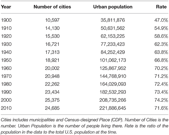
Table 1. Summary of U.S. population data.

TABLE 2

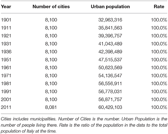
Table 2. Summary of population data for Italy.

TABLE 3

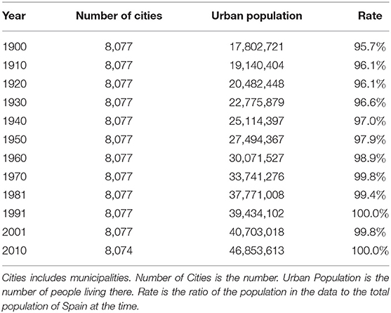
Table 3. Summary of population data for Spain.

In addition, in order to compare the initial value dependence of the growth rate distribution of the urban population, which is the main focus of this paper, we introduce the initial value dependence of the growth rate distribution of firms' sales, which is our previous study, in section 3. The analysis will use data from the Orbis 2016 edition, the world's largest corporate information database, provided by Bureau van Dijk. Specifically, we use the sales and establishment year data of 944,116 Japanese firms for which both 2013 and 2014 sales data exist. The most recent data in the 2016 edition of Orbis is from 2015, but since the database was in the process of being collected at the time it was available, and so was scarce (343, 473 firms), we used the largest data pair, 2014 (1, 029, 179 firms) and 2013 (1, 133, 993 firms), for our analysis. There were approximately 3.82 million firms in Japan in 2014, of which approximately 11, 000 were reported to be large firms, approximately 557, 000 to be medium-sized firms, and approximately 3, 252, 000 to be small-sized firms, according to the Small and Medium Business Administration of Japan. In Japan, small firms are defined by the number of employees under the Small and Medium-sized Enterprise Basic Law, which refers to firms with five employees or fewer in the retail, service, and wholesale industries and 20 or fewer in the manufacturing and other industries. Orbis is a comprehensive database of large and medium-sized Japanese firms, including small-sized firms whose sales are identifiable.

3. Short- and Long-term Properties of Firms

In this section, we briefly review our previous study of the initial dependence of the firms' sales growth rate distribution [29] and its long-term growth properties [30, 31] using new data we have. As mentioned in the previous section, our database contains sales data for 2013 and 2014 for 944, 116 Japanese firms. The minimum sales for 2013 was 1, 000 USD, and the maximum was 249, 799, 825 USD. To observe the initial value dependence of the growth rate (R = x₂₀₁₄/x₂₀₁₃) from 2013 sales (x₂₀₁₃) to 2014 sales (x₂₀₁₄), the initial values are divided into logarithmically equally sized bins as follows $x_{2013}\in [10^{0.5(n-1)},10^{0.5n})$ (n = 1, 2, ⋯ , 10). The number of firms in these 10 bins (n = 1, 2, ⋯ , 10) is 4, 355, 6, 426, 18, 354, 65, 866, 163, 052, 266, 023, 221, 607, 114, 967, 50, 459, and 20, 498, respectively. The number of firms greater than n = 10 is 12, 509. Although there are arbitrary ways to divide these bins, if a somewhat smooth growth-rate distribution is observed, the data are divided as finely as possible. When the bin is divided more finely than this way, a smooth growth-rate distribution is not observed, and when the bin is divided more roughly, the properties described below are hardly observed. However, it is confirmed by considering the case where the division of the bins is slightly changed from that described above, that the properties described below do not depend on the manner in which the bins are divided.

Figures 1, 2 are their conditional probability density functions. The horizontal axis represents the logarithmic growth rate r = log₁₀R, and the vertical axis represents the probability density function (PDF) q(r|n). Figure 1 shows that the smaller the initial value x₂₀₁₃ (the smaller n) is, the larger the positive growth rate, and that the negative growth rate is almost independent of the initial value. Figure 2 also shows that when the initial value x₂₀₁₃ is 10^2.5 thousand dollars or more (n is greater than or equal to 6), both the positive and negative growth-rate distributions are almost independent of the initial value. This property is called Gibrat's law [25, 26] and is observed in the large-scale range (Now x₂₀₁₃ is over 10^2.5 thousand dollars). On the other hand, our previous studies have shown that the non-Gibrat's property in Figure 1 is observed in the mid-scale range [28, 32, 33].

FIGURE 1

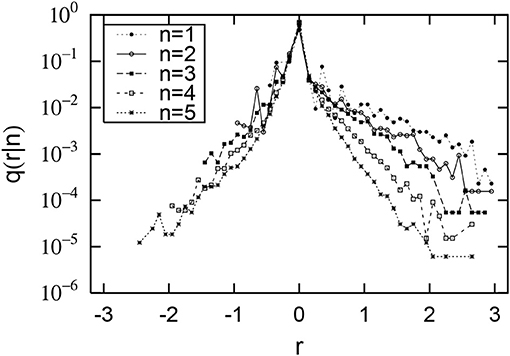
Figure 1. Distributions of sales growth rate of Japanese firms. The horizontal axis shows the logarithmic growth rate: $r={log}_{10}\frac{x_{2014}}{x_{2013}}$. The vertical axis shows its conditional probability density function: q(r|n). The initial sales value of x₂₀₁₃ for 2013 is divided into logarithmically equal sized bins: $x_{2013}\in [10^{0.5(n-1)},10^{0.5n})$ (n = 1, 2, ⋯ , 5).

FIGURE 2

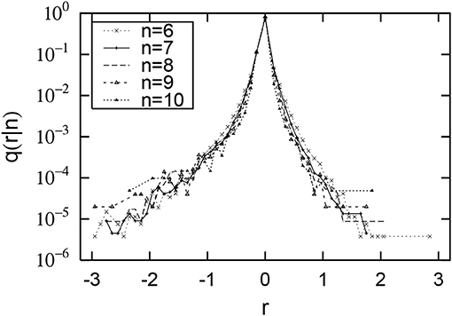
Figure 2. Distributions of sales growth rate of Japanese firms. The horizontal axis shows the logarithmic growth rate: $r={log}_{10}\frac{x_{2014}}{x_{2013}}$. The vertical axis shows its conditional probability density function: q(r|n). The initial sales value of x₂₀₁₃ for 2013 is divided into logarithmically equal sized bins: $x_{2013}\in [10^{0.5(n-1)},10^{0.5n})$ (n = 6, 7, ⋯ , 10).

In our previous study, we also reported that there is a long-term growth property in the dependence of the geometric mean of firms' sales regarding their age [30, 31]. Figure 3 depicts the firm age (t) dependency of the geometric mean sales (〈x_t〉) in 2014. Here, the firm age is defined as the year of establishment of the firm, e.g., t = 1. Figure 3, drawn on a semilogarithmic axis, shows that for the first 10 years, 〈x_t〉 rapidly grows following a power-law function:

$\begin{array}{ll}\langle x_t\rangle \propto t^{{\alpha }_{\text{sales}}t}& (1)\end{array}$

with α_sales = 0.53 ± 0.02 (the dotted line). Then, 〈x_t〉 gradually grows following an exponential function:

$\begin{array}{ll}\langle x_t\rangle \propto e^{{\beta }_{\text{sales}}t}& (2)\end{array}$

with β_sales = 0.014 ± 0.001 (the solid line). These values are measured by applying t = 1, 2, ⋯ , 10 for power-law growth (1) and t = 11, 12, ⋯ , 60 for exponential growth (2).

FIGURE 3

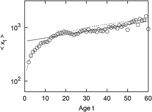
Figure 3. Dependence of geometric mean of Japanese firms' sales 〈x_t〉 in 2014 on firm age t.

Similar properties were confirmed not only in sales of Japanese firms but also in the number of employees of Japanese firms and sales and number of employees of French firms in previous studies [31]. Furthermore, we show by numerical simulation that these long-term growth properties are derived from the short-term growth properties mentioned above. The initial fast growth following the power-law function (1) is derived from the non-Gibrat's property, and the slow growth following the exponential function (2) is derived from Gibrat's law, using a stochastic process with numerical samples from real data.

4. Short- and Long-term Properties of Urban Population

The purpose of this study is to confirm whether the properties of short-term and long-term growth in firms' sales and the number of employees in our previous study are observed in an urban population. Tables 1–3 show that the number of cities in the United States is around 10, 000 to 25, 000, and those of Italy and Spain number around 8, 000. As in the previous section, if these initial values are placed in logarithmically equal-sized bins and a somewhat smooth growth-rate distribution is to be observed, there will be only a few bins, and it will be difficult to observe the properties of the previous section. In the United States, we have increased the number of pairs of data by overlaying all 11 pairs of data, such as 1900 − 1910, 1910 − 1920, and ⋯ , 2000 − 2010, and conducted the same analysis as in the previous section. This approach ignores changes in history over 110 years but has the advantage of being able to observe a macroscopic nature that is not influenced by the flow of history.

Using this method, pairs of 187,378 cities are created, each city's initial population is expressed as x_i, and the city's population 10 years later is expressed as x_i+10. The minimum value of x_i is 1 and the maximum value is 8, 008, 278. In the case of the United States, this small figure is recorded because it includes population data from Census-designed Places (CDP). To observe the dependence of the urban growth rate (R = x_i+10/x_i) on the initial value (x_i), we divide the initial value into logarithmically equidistant bins, as in the previous section, such as $x_i\in [10^{0.5(n-1)+2},10^{0.5n+2})$ (n = 1, 2, ⋯ , 7). The 7 bins contain the following cities: 34, 158 (n = 1), 56, 216 (n = 2), 41, 353 (n = 3), 22, 942 (n = 4), 10, 794 (n = 5), 3, 997 (n = 6), and 950 (n = 7). Number of cities less than n = 1 is 6, 278, and number of cities greater than n = 7 is 361. The same discussion as in the previous section applies to the arbitrariness of division into bins. Figure 4 shows the conditional PDF. The horizontal and vertical axes are the same as in the previous section. Figure 4 shows that the smaller the initial value x_i is (The smaller n is), the larger the negative growth rate is, and the positive growth rate is almost independent of the initial value. Surprisingly, this property is symmetrical with that observed in Figure 1. This property is explicitly confirmed in Figure 5, which shows the n-dependence of positive standard deviation (${\sigma }_{+}=\sqrt{{\Sigma }_{r>0}{r}^{2}q(r|n)}$) and negative one (${\sigma }_{-}=\sqrt{{\Sigma }_{r<0}{r}^{2}q(r|n)}$). Figure 5 shows that σ₊ is almost n independent, but σ₋ decreases depending on n, as approximated by

$\begin{array}{ll}{\sigma }_{-}\propto e^{-{\gamma }^{\text{US}}n}& (3)\end{array}$

with γ^US = 0.25 ± 0.03.

FIGURE 4

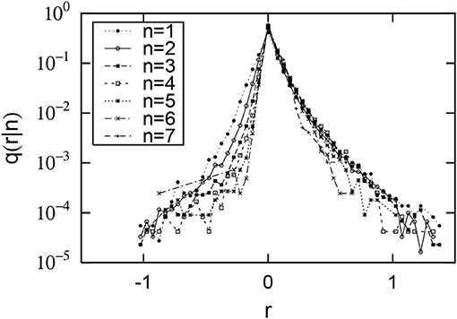
Figure 4. Distributions of urban population growth rates in the United States. The horizontal axis shows the logarithmic growth rate: $r={log}_{10}\frac{x_{i+10}}{x_i}$. The vertical axis shows its conditional probability density function: q(r|n). The initial population x_i is divided into logarithmically equal sized bins: $x_i\in [10^{0.5(n-1)+2},10^{0.5n+2})$ (n = 1, 2, ⋯ , 7).

FIGURE 5

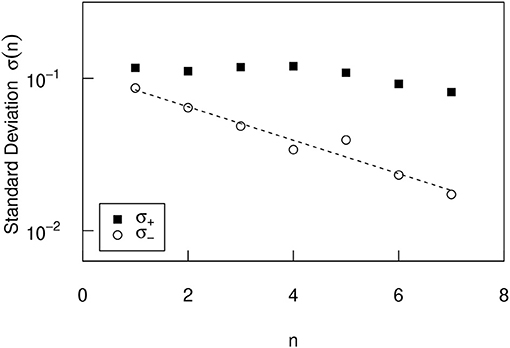
Figure 5. The n dependence of the positive and negative standard deviations σ_± of the conditional PDFs in the United States (Figure 4).

In the previous section, we observed the long-term property of the growth of the geometric mean of firms' sales depending on the firm age. With a slightly different perspective on urban population data, we observe the long-term property of the growth of the geometric mean of the urban population over the observable years by size of the initial population. Figure 6 shows the observed results for the urban population in the United States. The horizontal axis represents 1900, 1910, ⋯ , 2010 expressed as T = 1, 2, ⋯ , 12, respectively, and the vertical axis represents the geometric mean of the urban population in each year (〈x_T〉). In Figure 6, the original population of x₁ in 1900 (T = 1) is divided into logarithmically equally sized bins: $x_1\in [10^{m+1},10^{m+2})$ (m = 1, 2, 3), $x_1\ge 10^5$ (m = 4). The number of cities in each bin is 4, 593 (m = 1), 2, 482 (m = 2), 317 (m = 3), and 28 (m = 4). The number of cities less than m = 1 is 46. These totals are fewer than the 10,597 cities in 1900 because of the high frequency of urban renewal in the United States and the large number of cities that existed in 1900 but did not exist 110 years later. In Figure 6, which is the semilogarithmic axis, the optimum line is drawn by the least squares method for T = 1, 2, 3, 4. Figure 6 shows that for m = 1, 2 the whole period is approximated by an exponential function:

$\begin{array}{ll}\langle x_T\rangle \propto e^{{\beta }_{\text{city}}(m)T},& (4)\end{array}$

FIGURE 6

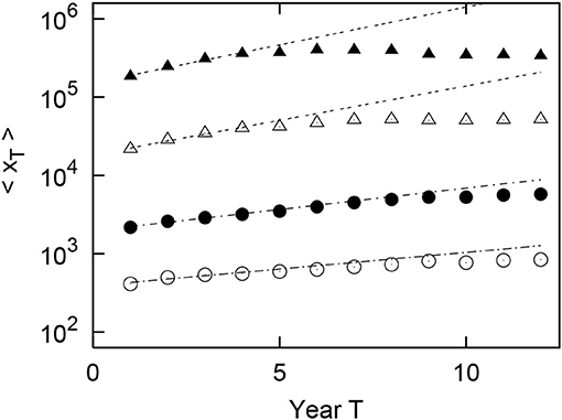
Figure 6. Geometric mean growth of the urban population in the United States from 1900 to 2010 (T = 1, 2, ⋯ , 12). The original population of x₁ in 1900 (T = 1) is divided into logarithmically equally sized bins: $x_1\in [10^{m+1},10^{m+2})$ (m = 1, 2, 3), $x_1\ge 10^5$ (m = 4). In the figure, ◦, •, △, and ▲each represent m = 1, 2, 3, and 4, respectively.

where β_city(m) is the index of urban growth corresponding to β_sales in Equation (2). Here, β_city(m) has a factor m because it varies depending on the bin containing the initial value x₁. On the other hand, at m = 3, 4, the exponential function is followed up to T = 4, after which the growth is negligible. Here, the exponents in U.S. ${\beta }_{\text{city}}^{\text{US}}(m)$ of the four straight lines (4) for m = 1, 2, 3, 4 in Figure 6 are evaluated as ${\beta }_{\text{city}}^{\text{US}}(1)=0.098\pm 0.026$, ${\beta }_{\text{city}}^{\text{US}}(2)=0.13\pm 0.01$, ${\beta }_{\text{city}}^{\text{US}}(3)=0.20\pm 0.02$, and ${\beta }_{\text{city}}^{\text{US}}(4)=0.22\pm 0.02$, respectively. These values are measured by applying T = 1, 2, 3, 4 for exponential growth (4). These indicate that ${\beta }_{\text{city}}^{\text{US}}(m)$ is an increasing function of m. In other words, the geometric mean growth of the urban population will be faster as the initial urban population size increases.

Similar analyses were conducted on urban population data in Italy and Spain. As with the initial value dependence of the urban population growth-rate distribution in the United States, the negative growth rate increases as the initial value x_i decreases, and the positive growth rate hardly depends on the initial value. These properties are expressed as positive and negative standard deviations σ_± in Figures 7, 8. In Figures 7, 8, as in the U.S., σ₊ is almost independent of n, and σ₋ has the same n dependency as in Equation (3). The parameters for Italy and Spain are evaluated as γ^IT = 0.26 ± 0.01 and γ^ES = 0.30 ± 0.06, respectively. In Italy, the number of (x_i, x_i+10) pair is 88, 303, and the seven bins contain the following cities: 2, 008 (n = 1), 14, 721 (n = 2), 36, 913 (n = 3), 26, 002 (n = 4), 6, 781 (n = 5), 1, 453 (n = 6), and 241 (n = 7). Number of cities less than n = 1 is 948, number of cities greater than n = 7 is 0. In Spain, the number of (x_i, x_i+10) pair is 87, 141, and the seven bins contain the following cities: 13, 979 (n = 1), 30, 333 (n = 2), 23, 407 (n = 3), 11, 980 (n = 4), 3, 496 (n = 5), 720 (n = 6), and 244 (n = 7). Number of cities less than n = 1 is 2, 924, number of cities greater than n = 7 is 302.

FIGURE 7

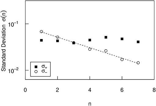
Figure 7. The n dependence of the positive and negative standard deviations σ_± of the conditional PDFs in Italy.

FIGURE 8

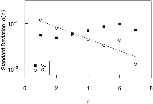
Figure 8. The n dependence of the positive and negative standard deviations σ_± of the conditional PDFs in Spain.

As in the United States, Figures 9, 10 shows the long-term properties of the geometric mean of the urban population growing with the passage of observable years by size of the original population in Italy and Spain. For Italy, each bin contains 1, 200 (m = 1), 6, 031 (m = 2), 467 (m = 3), and 11 (m = 4) cities. For Spain, each bin contains 4, 202 (m = 1), 3, 375 (m = 2), 211 (m = 3), and 6 (m = 4) cities. The number of cities less than m = 1 is 2 in Italy and 6 in Spain. In Figures 9, 10 on the semilogarithmic axis, the optimum line is drawn by the least squares method for T = 1, 2, ⋯ , 8. From these optimal straight lines, we confirm that the geometric mean of urban population grows approximately exponentially over almost all periods for the case of m = 1, 2, 3, and 4. Here, the exponents in Italy ${\beta }_{\text{city}}^{\text{IT}}(m)$ of the four straight lines (4) for m = 1, 2, 3, 4 in the Italian long-term growth Figure 9 are evaluated as ${\beta }_{\text{city}}^{\text{IT}}(1)=-0.0071\pm 0.0058$, ${\beta }_{\text{city}}^{\text{IT}}(2)=0.0055\pm 0.0071$, ${\beta }_{\text{city}}^{\text{IT}}(3)=0.055\pm 0.003$, and ${\beta }_{\text{city}}^{\text{IT}}(4)=0.14\pm 0.01$, respectively. The exponents in Spain ${\beta }_{\text{city}}^{\text{ES}}(m)$ of the four straight lines (4) for m = 1, 2, 3, 4 in the Spanish long-term growth Figure 10 are evaluated as ${\beta }_{\text{city}}^{\text{ES}}(1)=-0.030\pm 0.017$, ${\beta }_{\text{city}}^{\text{ES}}(2)=0.016\pm 0.009$, ${\beta }_{\text{city}}^{\text{ES}}(3)=0.085\pm 0.003$, and ${\beta }_{\text{city}}^{\text{ES}}(4)=0.18\pm 0.01$, respectively. These values are measured by applying T = 1, 2, ⋯ , 8 for exponential growth (4). As in the U.S., ${\beta }_{\text{city}}^{\text{IT}}(m)$ and ${\beta }_{\text{city}}^{\text{ES}}(m)$ are also increasing functions of m. Significantly different from the U.S. is that the index β_city(1) for m = 1 becomes negative, i.e., for m = 1, the geometric mean of the urban population 〈x_T〉 decreases depending on T in Italy and Spain.

FIGURE 9

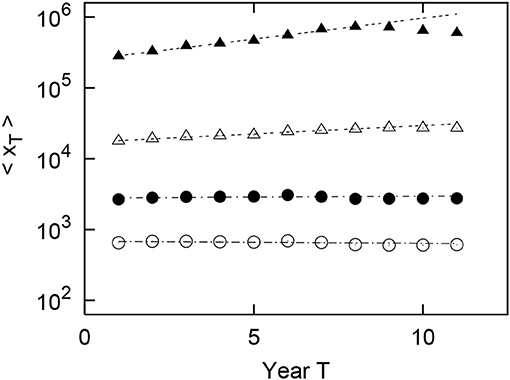
Figure 9. Geometric mean growth of the urban population in Italy from 1901 to 2001 (T = 1, 2, ⋯ , 11). The original population of x₁ in 1901 (T = 1) is divided into logarithmically equally sized bins: $x_1\in [10^{m+1},10^{m+2})$ (m = 1, 2, 3), $x_1\ge 10^5$ (m = 4). In the figure, ◦, •, △, and ▲each represent m = 1, 2, 3, and 4, respectively.

FIGURE 10

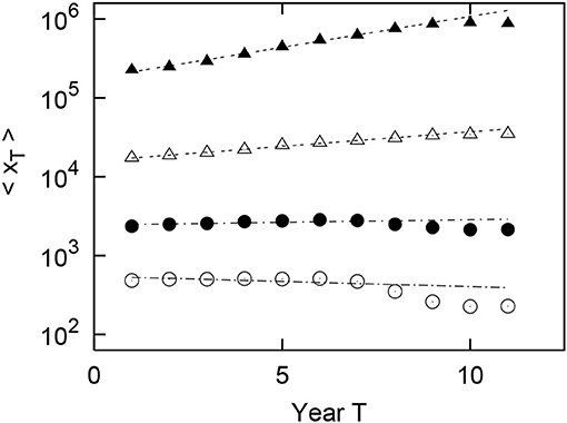
Figure 10. Geometric mean growth of the urban population in Spain from 1900 to 2001 (T = 1, 2, ⋯ , 11). The original population of x₁ in 1900 (T = 1) is divided into logarithmically equally sized bins: $x_1\in [10^{m+1},10^{m+2})$ (m = 1, 2, 3), $x_1\ge 10^5$ (m = 4). In the figure, ◦, •, △, and ▲each represent m = 1, 2, 3, and 4, respectively.

5. Simulation of Long-term Growth Property

In the previous section, we observed the dependence of the short-term growth-rate distribution on the initial value and observed the properties of long-term growth. With respect to the initial value dependence of the short-term growth rate, it was observed that the probability of a decrease in the urban population increases as the initial population decreases, and that the probability of an increase in the urban population does not depend on the initial population in any of the countries in which the urban population data were analyzed. As for long-term growth, it was confirmed that the geometric mean of the urban population 〈x_T〉 grew exponentially $e^{{\beta }_{\text{city}}(m)T}$ as in Equation (4), depending on the year T = (1, 2, ⋯ ). In Italy and Spain, an exponential decline (${\beta }_{\text{city}}^{\text{IT}}(1),{\beta }_{\text{city}}^{\text{ES}}(1)<0$) was also observed for small (m = 1) original (T = 1) urban populations ($x_1\in [10^2,10^3)$). Collectively, we observed that the larger the original urban population x₁ (the larger the m), the larger the exponent of the exponential function β_city(m), which indicates the rate of growth. It was also observed that as large cities grew, their growth slowed and stopped.

This section uses simulations to show how these short- and long-term growth properties are related. Specifically, we use data sampled from the short-term growth-rate distribution to grow cities with different initial values and confirm whether the long-term growth has the properties observed in the real data.

Since it is important to adopt a non-Gibrat's property that the growth-rate distribution differs depending on the initial value, the simulation was designed as follows. First, we divided the initial city population x_T into eight bins: $x_T\in [1,10^2)$, $x_T\in [10^{0.5(n-1)+2},10^{0.5n+2})$ (n = 1, 2, ⋯ , 6), and $x_T\in [10^5,\infty )$. The first and last bins differ from those in the previous section for the initial dependence of the growth-rate distribution. The first bin is needed if the city population is smaller than 10² in the simulation. The last bin removes the upper limit 10^5.5 in the empirical data analysis to increase the number of data items in the bin. A bin corresponding to an initial value x_T is selected from these eight bins, and a growth rate R is extracted at random from the bin, and each urban population is grown by x_T+1 = Rx_T to grow each urban population. In the simulation, this step is repeated 10 times to obtain x₁, x₂, ⋯ , x₁₁.

We confirm that this growth depends on the original urban population size x₁ as follows. From the 1900 urban population, for seven cases with different original values, we randomly extracted the population of 10, 000 with repetition: $x_1\in [10^{0.5(m-1)+2},10^{0.5m+2})$ (m = 1, 2, ⋯ , 7). The 10-step growth of the geometric mean of the urban population classified by the seven different original values is depicted in Figure 11 for the United States and Figure 12 for Italy. The results for Spain are so similar to those for Italy that they have been omitted. In Figures 11, 12, as in Equation (4), it is confirmed that the geometric mean of the urban population 〈x_T〉 grows as an exponential function of step T: $\langle x_T\rangle \propto e^{{\beta }_{\text{sim}}(m)T}$. In the following, the exponent of exponential growth observed in the simulation is expressed as β_sim(m). The exponent β_sim(m) increases with increasing m initially but decreases with increasing m.

FIGURE 11

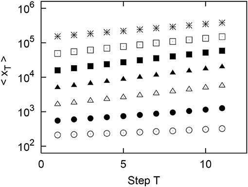
Figure 11. Results of simulation of the growth of the geometric mean of the urban population using values randomly sampled from real data in the United States. Original (T = 1) populations x₁ are divided into logarithmically equally sized bins: $x_1\in [10^{0.5(m-1)+2},10^{0.5m+2})$ (m = 1, 2, ⋯ , 7). Points in the figure indicate m = 1, 2, ⋯ , 7 in order from the bottom.

FIGURE 12

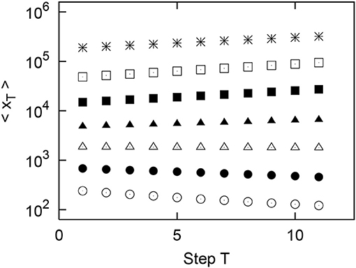
Figure 12. Results of simulation of the growth of the geometric mean of the urban population using values randomly sampled from real data in Italy. Original (T = 1) populations x₁ are divided into logarithmically equally sized bins: $x_1\in [10^{0.5(m-1)+2},10^{0.5m+2})$ (m = 1, 2, ⋯ , 7). Points in the figure indicate m = 1, 2, ⋯ , 7 in order from the bottom.

Figures 13–15 show the correlation of this index β_sim(m) and m in the U.S., Italy, and Spain, respectively. In these countries, β_sim(m) initially increased linearly with m. The exponents are approximated by ${\beta }_{\text{sim}}^{\text{US}}(m)=0.041m+0.001$ in the U.S., ${\beta }_{\text{sim}}^{\text{IT}}(m)=0.033m-0.102$ in Italy, and ${\beta }_{\text{sim}}^{\text{ES}}(m)=0.060m-0.201$ in Spain. Here we consider the optimal line for the first 3 n in Figure 13 and the first 5 n in Figures 14, 15. In Italy and Spain, the intercept of these linear relationships is negative, so β_sim(m) becomes negative when m is small. The value of the index β_sim obtained from the simulation results is closer to the value of β_city(m) measured from the actual city growth. However, they are not exactly the same and do not have to be because they are simulated over different time periods. Importantly, the m dependency of β results from the non-Gibrat's property. Because, it can be confirmed that the m dependency of β_sim does not occur by simulation without the procedure of selecting the growth rate R from eight n bins divided by the initial value x_T.

FIGURE 13

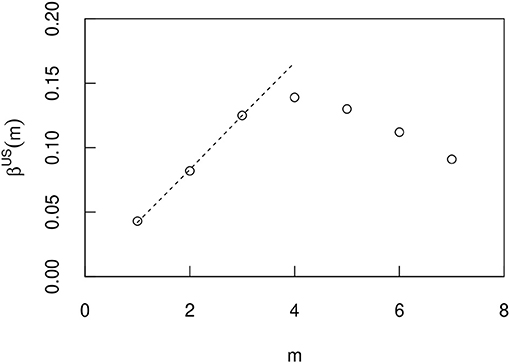
Figure 13. The m dependence of the exponent β^US(m) when the T dependence of the geometric mean 〈x_T〉 is approximated by an exponential function e^βUS(m)T in a US simulation (Figure 11). The errors are so small that they do not appear in the figure, and they are therefore omitted.

FIGURE 14

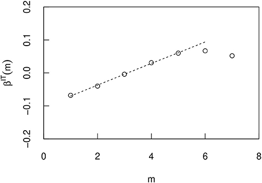
Figure 14. The m dependence of the exponent β^IT(m) when the T dependence of the geometric mean 〈x_T〉 is approximated by an exponential function e^βIT(m)T in a Italy simulation (Figure 12). The errors are so small that they do not appear in the figure, and they are therefore omitted.

FIGURE 15

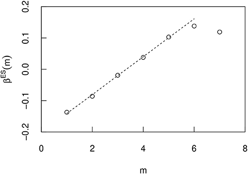
Figure 15. The m dependence of the exponent β^ES(m) when the T dependence of the geometric mean 〈x_T〉 is approximated by an exponential function e^βES(m)T in a Spain simulation. The errors are so small that they do not appear in the figure, and they are therefore omitted.

6. Conclusion

This paper uses census municipal population data (these are collectively called urban populations in this paper) for the United States, Italy, and Spain to analyze the statistical properties of their 10-year growth (short-term growth). As a result, it was confirmed that the smaller the initial urban population is, the greater the probability that the urban population will decrease, and that the probability that the urban population will increase does not depend on the initial urban population. We call this the non-Gibrat's property of the urban population. We also observed the statistical properties of long-term growth of urban populations in each country over 100 years. Specifically, we identified the following properties by observing the geometric mean of logarithmically equal sized bins of the oldest urban population in the data used in the analysis.

1. The average urban population increases or decreases exponentially with time.

2. The smaller the initial average urban population, the smaller the exponent, which can be negative in Italy and Spain.

3. When the average urban population is large, exponential growth may stop.

We conducted the following simulations to clarify the relationship between these short- and long-term properties. First, the original urban population was randomly extracted from the oldest urban population in the analysis, and using short-term growth data, they were grown by 10 steps. What is important here is that the growth rate varies according to the size of the initial urban population according to the non-Gibrat's property. As a result, it was confirmed that almost all of the above properties observed in real data for 100 years were reproduced. Specifically, the following long-term properties were confirmed.

4. The geometric mean of the urban population grows or declines exponentially over time.

5. The index increases with the size of the original urban population.

6. However, when the original urban population is very large, the index turns to decline.

The property 6. is considered to be the property 3. smoothed by simulation.

Finally, we consider how the short-term properties leads to the long-term properties 1. and 2. First, we assume that the definition of the growth rate approximately holds for the geometric mean. Furthermore, the growth rate does not change approximately over a period of around 100 years. In this case, it is easy to derive that the geometric mean of the urban population grows exponentially, and that the index is the geometric mean of the growth rate minus one. From the non-Gibrat's property observed in the short-term growth rate, it can be concluded that the smaller the urban population size, the smaller the geometric mean of the growth rate, and therefore the smaller the index of exponential growth. In this way, the non-Gibrat's property of short-term growth can be interpreted as being linked to the long-term growth property. In the case of firm sales, the non-Gibrat's property observed in the initial value dependence of the distribution of short-term growth rates produced the firms' initial rapid exponential growth. In the case of urban populations, on the other hand, the non-Gibrat's property controls the rate of long-term slow exponential growth through the mechanisms described above. It is very interesting that the different non-Gibrat's properties of firm sales and urban population lead to different long-term growths.

It was predictable that the distribution of the short-term growth rate in the mid-size range was dependent on the initial value, because the power-law distribution in the large-size range was collapsed in the mid-size range in both firm sales and urban population. In this study, we found that the urban population has a property that is completely opposite to the initial value dependence of the distribution of the short-term growth rate of firm sales, as described in 1. to 3. above. The decline in the urban population will be a policy issue. In the macro view of this paper, the solution is to merge cities with smaller populations. In Italy and Spain, cities with populations generally below tens of thousands tend to decline. This figure may serve as an indicator for policymaking. However, it is necessary to carefully examine the causal relationship between such figures and the results of the merger policy. This is a future issue.

In this paper, we derive these results from three data analyses, the U.S., Italy, and Spain Census. The remaining challenge is to clarify the relationship between the short-term growth parameter γ and the long-term growth parameter β. Since γ in the three countries matches within the margin of error, this may be a universal nature. It is also possible that γ is involved in the correlation between β and m. We are looking to solve this problem in the near future by analyzing the urban population data we are trying to obtain in France and Germany.

This paper discusses the macro-statistical properties of urban population. This discussion does not take into account the microscopic nature of individuals at all, and it is thus not possible to answer why the non-Gibrat's property occurs. In order to develop the results of this paper and better understand the nature of urban population, we need to take into account the microscopic perspective of human movement between cities. On an individual level, it is a likely scenario that people tend to move away from less populated cities because they are inconvenient and difficult to live in. It is also conceivable that the population of cities with too many people will not increase further because they are difficult to live in. In order to construct a theory incorporating such properties, a microscopic view of the network structure will be important [34, 35]. This is an important issue that should be addressed in the future.

Data Availability Statement

Publicly available datasets were analyzed in this study. This data can be found here: the census information of the municipal population data of the United States, Italy, and Spain.

Author Contributions

AI and SF conceived of the presented idea. AI developed the theory and performed the computations. AR verified the analytical methods. TM encouraged AI to investigate non-Gibrat's property and supervised the findings of this work. All authors discussed the results and contributed to the final manuscript.

Funding

This study was supported by JSPS KAKENHI Grant Numbers 17K01277, 16H05904, 18H05217, ROIS NII Open Collaborative Research 2019-FS01, the Obayashi Foundation, The Okawa Foundation for Information and Telecommunications, and ECO2017-82246-P of the Spanish Ministerio de Economía y Competitividad and ADETRE Reference Group of Gobierno de Aragón.

Conflict of Interest

The authors declare that the research was conducted in the absence of any commercial or financial relationships that could be construed as a potential conflict of interest.

Acknowledgments

The authors thank Dr. Tsutomu Watanabe with whom much of this work was discussed and Drs. Rafael González-Val, Luis Lanaspa, and Fernando Sanz-Gracia for the databases that we have used in this paper.

References

1. Mantegna RN, Stanley HE. An Introduction to Econophysics: Correlation and Complexity in Finance. New York, NY: Cambridge University Press (1999).

Google Scholar

2. Pareto V. Cours d'Économie Politique. London: Macmillan (1897).

Google Scholar

3. Newman M. Power laws, Pareto distributions and Zipf's law. Contemp Phys. (2005) 46:323–51. doi: 10.1080/00107510500052444

CrossRef Full Text | Google Scholar

4. Clauset A, Shalizi CR, Newman M. Power-law distributions in empirical data. SIAM Rev. (2009) 51:661–703. doi: 10.1137/070710111

CrossRef Full Text | Google Scholar

5. Saichev A, Malevergne Y, Sornette D. Theory of Zipf's Law and Beyond. New York, NY: Springer (2009).

Google Scholar

6. Aoyama H, Fujiwara Y, Ikeda Y, Iyetomi H, Souma W. Econophysics and Companies -Statistical Life and Death in Complex Business Networks. New York, NY: Cambridge University Press (2010).

Google Scholar

7. Anazawa M, Ishikawa A, Suzuki T, Tomoyose M. Fractal structure with a typical scale. Phys A. (2004) 335:616–28. doi: 10.1016/j.physa.2003.12.006

CrossRef Full Text | Google Scholar

8. Ishikawa A, Suzuki T. Relations between a typical scale and averages in the breaking of fractal distribution. Phys A. (2004) 343:376–92. doi: 10.1016/j.physa.2004.06.060

CrossRef Full Text | Google Scholar

9. Reed WJ. On the rank-size distribution for human settlements. J Reg Sci. (2002) 42:1–17. doi: 10.1111/1467-9787.00247

CrossRef Full Text | Google Scholar

10. Reed WJ. The Pareto law of incomes–an explanation and an extension. Phys A Stat Mech Appl. (2003) 319:469–86. doi: 10.1016/S0378-4371(02)01507-8

CrossRef Full Text | Google Scholar

11. Reed WJ, Jorgensen M. The double Pareto-lognormal distribution -a new parametric model for size distributions. Commun Stat Theor Methods. (2004) 33:1733–53. doi: 10.1081/STA-120037438

CrossRef Full Text | Google Scholar

12. Eeckhout J. Gibrat's law for (all) cities. Am Econ Rev. (2004) 94:1429–51. doi: 10.1257/0002828043052303

CrossRef Full Text | Google Scholar

13. González-Val R. The evolution of US city size distribution from a long-term perspective (1900-2000). J Reg Sci. (2010) 50:952–72. doi: 10.1111/j.1467-9787.2010.00685.x

CrossRef Full Text | Google Scholar

14. Giesen K, Zimmermann A, Suedekum J. The size distribution across all cities–double Pareto lognormal strikes. J Urban Econ. (2010) 68:129–37. doi: 10.1016/j.jue.2010.03.007

CrossRef Full Text | Google Scholar

15. Giesen K, Suedekum J. City age and city size. Eur Econ Rev. (2014) 71:193–208. doi: 10.1016/j.euroecorev.2014.07.006

CrossRef Full Text | Google Scholar

16. González-Val R, Lanaspa L, Sanz-Gracia F. New evidence on Gibrat's law for cities. Urban Stud. (2013) 51:93–115. doi: 10.1177/0042098013484528

CrossRef Full Text | Google Scholar

17. González-Val R, Lanaspa L, Sanz-Gracia F. Gibrat's law for cities, growth regressions and sample size. Econ Lett. (2013) 118:367–9. doi: 10.1016/j.econlet.2012.11.020

CrossRef Full Text | Google Scholar

18. González-Val R, Ramos A, Sanz-Gracia F, Vera-Cabello M. Size distributions for all cities: which one is best? Pap Reg Sci. (2015) 94:177–96. doi: 10.1111/pirs.12037/full

CrossRef Full Text | Google Scholar

19. Puente-Ajovín M, Ramos A. On the parametric description of the French, German, Italian and Spanish city size distributions. Ann Reg Sci. (2015) 54:489–509. doi: 10.1007/s00168-015-0663-3

CrossRef Full Text | Google Scholar

20. Luckstead J, Devadoss S. Pareto tails and lognormal body of US cities size distribution. Phys A Stat Mech Appl. (2017) 465:573–8. doi: 10.1016/j.physa.2016.08.061

CrossRef Full Text | Google Scholar

21. Luckstead J, Devadoss S, Danforth D. The size distributions of all Indian cites. Phys A Stat Mech Appl. (2017) 465:573–8. doi: 10.1016/j.physa.2017.01.065

CrossRef Full Text | Google Scholar

22. Kwong HS, Nadarajah S. A note on “Pareto tails and lognormal body of US cities size distribution”. Phys A Stat Mech Appl. (2019) 513:55–62. doi: 10.1016/j.physa.2018.08.073

CrossRef Full Text | Google Scholar

23. Bǎncescu I, Chivu L, Preda V, Puente-Ajovín M, Ramos A. Comparisons of log-normal mixture and Pareto tails, GB2 or log-normal body of Romania's all cities size distribution. Phys A Stat Mech Appl. (2019) 526:121017. doi: 10.1016/j.physa.2019.04.253

CrossRef Full Text | Google Scholar

24. Su HL. On the city size distribution: a finite mixture interpretation. J Urban Econ. (2020) 116:103216. doi: 10.1016/j.jue.2019.103216

CrossRef Full Text | Google Scholar

25. Gibrat R. Les Inegalites Economiques. Paris: Sirey (1932).

Google Scholar

26. Sutton J. Gibrat's Legacy. J Econ Liter. (1997) 35:40–59.

Google Scholar

27. Li R, Dong L, Zhang J, Wang X, Wang WX, Di Z, et al. Simple spatial scaling rules behind complex cities. Nat Commun. (2017) 8:1841. doi: 10.1038/s41467-017-01882-w

PubMed Abstract | CrossRef Full Text

28. Ishikawa A. Derivation of the distribution from extended Gibrat's law. Phys A. (2006) 367:425–34. doi: 10.1016/j.physa.2005.12.005

CrossRef Full Text | Google Scholar

29. Ishikawa A, Fujimoto S, Mizuno T. Shape of growth-rate distribution determines the type of Non-Gibrat's Property. Phys A. (2011) 390:4273–85. doi: 10.1016/j.physa.2011.06.043

CrossRef Full Text | Google Scholar

30. Ishikawa A, Fujimoto S, Mizuno T, Watanabe T. Firm growth function and extended-Gibrat's property. Adv Math Phys. (2016) 2016:9303480. doi: 10.1155/2016/9303480

CrossRef Full Text | Google Scholar

31. Ishikawa A, Fujimoto S, Mizuno T, Watanabe T. Long-term firm growth properties derived from short-term laws of sales and number of employees in Japan and France. Evol Inst Econ Rev. (2016) 2016:409–22. doi: 10.1007/s40844-016-0055-0

CrossRef Full Text | Google Scholar

32. Ishikawa A. The uniqueness of firm size distribution function from tent-shaped growth rate distribution. Phys A. (2007) 383:79–84. doi: 10.1016/j.physa.2007.04.089

CrossRef Full Text | Google Scholar

33. Tomoyose M, Fujimoto S, Ishikawa A. Non-Gibrat's law in the middle scale region. Prog Theor Phys Suppl. (2009) 179:114–22. doi: 10.1143/PTPS.179.114/1914937

CrossRef Full Text | Google Scholar

34. Wang J, Li C, Xia C. Improved centrality indicators to characterize the nodal spreading capability in complex networks. Appl Math Comput. (2018) 334:388–400. doi: 10.1016/j.amc.2018.04.028

CrossRef Full Text | Google Scholar

35. Li C, Wang L, Sun S, Xia C. Identification of influential spreaders based on classified neighbors in real-world complex networks. Appl Math Comput. (2018) 320:512–23. doi: 10.1016/j.amc.2017.10.001

CrossRef Full Text | Google Scholar